
Diagnosing Schizophrenia Using Effective Connectivity of Resting-State EEG Data
by
 ,
,
Claudio Ciprian
1, 
Kirill Masychev
1,
Maryam Ravan
2,*,
Akshaya Manimaran
2 and
AnkitaAmol Deshmukh
1 1
Department of Computing Science, New York Institute of Technology, New York, NY 10023, USA
2
Department of Electrical and Computer Engineering, New York Institute of Technology, New York, NY 10023, USA
*
Author to whom correspondence should be addressed.
Algorithms 2021, 14(5), 139; https://0-doi-org.brum.beds.ac.uk/10.3390/a14050139
Submission received: 17 December 2020
/
Revised: 21 April 2021
/
Accepted: 22 April 2021
/
Published: 27 April 2021
(This article belongs to the Special Issue Machine Learning Algorithms for Biomedical Signal Processing)
Abstract
:Schizophrenia is a serious mental illness associated with neurobiological deficits. Even though the brain activities during tasks (i.e., P300 activities) are considered as biomarkers to diagnose schizophrenia, brain activities at rest have the potential to show an inherent dysfunctionality in schizophrenia and can be used to understand the cognitive deficits in these patients. In this study, we developed a machine learning algorithm (MLA) based on eyes closed resting-state electroencephalogram (EEG) datasets, which record the neural activity in the absence of any tasks or external stimuli given to the subjects, aiming to distinguish schizophrenic patients (SCZs) from healthy controls (HCs). The MLA has two steps. In the first step, symbolic transfer entropy (STE), which is a measure of effective connectivity, is applied to resting-state EEG data. In the second step, the MLA uses the STE matrix to find a set of features that can successfully discriminate SCZ from HC. From the results, we found that the MLA could achieve a total accuracy of 96.92%, with a sensitivity of 95%, a specificity of 98.57%, precision of 98.33%, F1-score of 0.97, and Matthews correlation coefficient (MCC) of 0.94 using only 10 out of 1900 STE features, which implies that the STE matrix extracted from resting-state EEG data may be a promising tool for the clinical diagnosis of schizophrenia.
1. Introduction
Schizophrenia is a severe neuropsychiatric disorder affecting approximately 20 million people worldwide according to the World Health Organization (WHO) report [1,2]. Schizophrenia is characterized by noticeable psychotic symptoms including hallucinations, delusions, reduction in performance, and thought disorder. Based on neuroimaging evidence on structural, functional, and effective brain connectivity, a core deficit of schizophrenia can be proposed as the failure of effective functional integration within and between brain areas [3].
Several studies proved alterations in functional connectivity (FC) in patients with schizophrenia (SCZs) in comparison to healthy controls (HCs) in response to external cognitive or sensorimotor stimulation [4,5,6]. However, resting-state electroencephalography (EEG) FC reflects the intrinsic inter-neuronal connections in specific circuits such as the default mode network (DMN) that are attenuated or interrupted during cognitive or sensorimotor tasks [7]. Therefore, investigating resting-state brain connectivity may reveal an intrinsic functional disintegration of brain regions for SCZ.
Machine learning algorithms (MLAs) have been widely used in applications related to neuroscience and psychiatry (e.g., [6,8,9,10]). Recently, there has been an increasing number of studies that use MLAs to diagnose schizophrenia based on resting-state EEG patterns. In Table 1, we highlighted the outcomes of the fourteen most recent studies in this area with the highest classification accuracy. Boostani et al. [11] extracted several features including band power, autoregressive (AR) model parameters, and a fractal dimension from the recorded resting-state EEG data (286 features). They applied different classifiers to extracted features to classify the two groups of 13 SCZs and 18 HCs. They achieved the highest classification accuracy of 87.51% using a boosted version of direct linear discriminant analysis (BDLDA). Khodayari et al. [12] used various statistical quantities such as the spectral coherence between all electrode pairs, the absolute and relative power spectral densities (PSDs), the left-to-right hemisphere power ratios, the anterior-to-posterior power ratios, and mutual information between all electrode pairs at the frequency range of 4–36 Hz with 1 Hz resolution to classify 40 SCZs, 64 patients with major depressive disorder (MDD), and 91 HCs. Using 42 most discriminating features and the mixture of factor analysis (MFA) for classification, they achieved the classification accuracy of 87.1%. Sabeti et al. [13] applied MLA to 20 SCZs and 20 HCs. They first selected the most informative EEG electrodes using mutual information techniques. Several features including autoregressive model parameters, fractal dimension, and band power were used for classification. Using 20 EEG electrodes, the total number of features was 300 for each 1 s window of EEG data, which resulted in 300 × 120 = 36,000 features for 2-min recorded data for each participant. Then, they employed genetic programming (GP) to select the best features. GP is a technique of creating algorithms that can program themselves by mimicking natural biological breeding and evolution. GP starts from a population of random programs and lets the machine automatically search among the space of all programs and breed the most successful or suitable ones in new generations [14]. They obtained the highest classification accuracy of 91.94% using the Adaboost classifier with 80 features. Thilakvathi et al. [15] considered Shannon entropy and Higuchi’s fractal dimension at five lobes of frontal, central, parietal, temporal, and occipital (in total 10 features) as their selected features to compare the complexity of a resting-state EEG signal for SCZ and HC using 55 SCZs and 23 HCs. Using these 10 features, the support vector machine (SVM) classifier obtained the highest accuracy of 80% using 20% of the data in each group for testing. Liu et al. [16] applied MLA to the resting-state EEG data of 40 clinically high-risk individuals (CHRs), 40 SCZs, and 40 HCs to investigate whether the EEG characteristics of these three groups can differentiate CHRs and SCZs from each other and from HCs. Using von Neumann Entropy as the linear eigenvalue statistics (LES) feature for each window of 200 EEG data samples (1500 features in total for 300,000 EEG data samples), they showed that the SVM classifier achieved the highest classification performance of 91.16% for classifying SCZs from HCs and 73.31% for classifying the three classes of CHRs, SCZs, and HCs. Phang et al. [17] proposed a deep multi-domain connectome convolutional neural network (MDC-CNN) framework for classifying the resting-state EEG-derived brain connectome in SCZs and HCs. By combining three connectivity features of (1) time-domain vector autoregressive (VAR) model coefficients; (2) the frequency-domain partial directed coherence (PDC); and (3) the network topology-based complex network (CN) measures (2730 features), they achieved the classification performance of 93.06% for classifying 45 SCZs and 39 HCs. Li et al. [18] used the inherent spatial pattern of the network (SPN) features extracted from resting-state EEG data to classify 19 SCZs and 23 HCs. Using four SPN filters, they achieved the highest accuracy of 88.10% with the SVM classifier.
Oh et al. [19] applied an 11-layer CNN model to differentiate resting-state EEGs of 14 SCZs and 14 HCs with deep learning. A total of 1142 EEG segments were used for each subject, where each segment consisted of 6250 time samples and 19 electrodes. Therefore, the total number of sampling points was 1142 × 6250 × 19 = 135,612,500. The most significant features were then automatically extracted by the CNN. Their proposed model achieved classification accuracies of 81.26%. This dataset (14 SCZs and 14 HCs) has been used in four more studies to diagnose schizophrenia [20,21,22,23]. In [20], Jahmunah et al. first segmented the EEG data for each subject into segments of 25 sec. Therefore, they obtained 516 segments for HC and 626 segments for SCZ. They extracted 157 non-linear features such as the largest Lyapunov exponent, Kolmogorov–Sinai entropy, Hjorth complexity and mobility, Kolmogorov complexity, bispectrum, and permutation entropy. The optimal 14 features were then selected and applied to various classifiers, where the best performance belonged to the SVM classifier with an accuracy of 92.91%. In [21], Buettner et al. used 200 power bands within a range of 0.5 Hz each as features that applied to a random forest (RF) classifier. Using 499 1-min samples for all 28 subjects (375 for training and 124 for evaluation), they yield an accuracy of 96.77%. In [22], Racz et al. used 21 dynamic features of dynamic FC (DFC) at delta frequency bands (0.5–4 Hz) such as its entropy and multifractal properties to classify the two groups. They achieved a classification performance of 89.29% using an RF classifier. In [23], Goshvarpour et al. selected non-linear features including complexity (Cx), Higuchi fractal dimension (HFD), and Lyapunov exponent and the fusion of these features using five different combination rules (R1: summation, R2: product, R3: division, R4: weighted sum using F-values, and R5: weighted sum using information gain ratio (IGR) rules) for 19 EEG electrodes. Using the probabilistic neural network (PNN) classifier and the R3 rule features, they achieved a classification performance of 100%.
Baradits et al. [24] investigated whether abnormalities in microstates, quasi-stable electrical fields in the EEG data, can be used to classify SCZs and HCs. They used four microstates (microstate A: auditory network; microstate B: visual network; microstate C: salience network; and microstate D: fronto–parietal network) and obtained 24 features including basic microstate features (microstate average duration, occurrence per second, full coverage of the time, 4 × 3 = 12 features) and the microstates transition probabilities (12 features). Using 14 out of 24 features that demonstrate significant differences between SCZ and HC and SVM classifier, they yield 82.7% accuracy for classifying 70 SCZs and 75 HCs. Kim et al. [25] recruited 119 SCZs and 119 HCs in their study. They obtained the source-level cortical FC network, where minimum norm estimation (MNE) was used to estimate the time series of source activity and the phase-locking value was used for calculating FC. Values of the clustering coefficient (CC) and path length for the cortical functional network were then used as selected features. Using the linear discriminant analysis (LDA) classifier, the best classification performance was 80.66% by choosing 27 optimal features.
In eight of these studies, a small dataset of SCZs and HCs was analyzed [11,13,18,19,20,21,22,23], which limits the power and applicability of the MLAs and deep learning algorithms. Using databases with larger data samples would allow having sufficient training data to adjust the model parameters more accurately and therefore increase the generalizability/reliability of the model, i.e., the performance on previously unseen data. Particularly when the selected features display significant variability, a larger training dataset is required to have a reliable classification performance. Furthermore, the sample size (Ns) to the number of features (Nf) ratio in some studies [11,12,13,16,20,21,22,23] is much lower than the rule of 10:1, or Nf is larger than the square root of Ns, which are referred to as the rules of preventing over-fitting (good quality) [24]. Finally, two of these studies [17,19] used deep learning algorithms, which are more complex compared to traditional MLAs and therefore require more training data to be reliable. Furthermore, complex feature engineering (the process of using domain knowledge to extract features from raw data) increases the difficulty to interpret the model [26]. Hence, only three studies [15,24,25] meet the optimal properties of a high to very high sample size (Ns > 100) and Nf to Ns ratio rules; however, the classification accuracy of these studies is less than 85%.
The objective of this study is to develop a new MLA based on effective connectivity (EC) measurements to study distinguishing characteristics between schizophrenics and healthy brains using a small set of selected features. FC reflects the statistical dependencies of signals from different brain regions as typically revealed by cross-correlation, coherency, or phase lag index measures. In contrast, EC measures the causal influences that a neural unit applies over another, which defines the mechanisms of neuronal coupling much more precisely than FC [27].
The method to measure EC must fulfill four criteria to be useful for measuring connectivity between brain areas [28], which are (1) independence from any a priori definitions and models; (2) ability to detect strong non-linear interactions across all levels of the brain function from the mechanism of action potential generation in neurons to psychometric functions; (3) the ability to detect EC even with a wide interaction delay between the two signals, reflecting signal transmission through multiple pathways or over complex axonal networks; and (4) robustness against linear cross-talk between signals. Transfer entropy (TE), a model-free statistic that can measure the directed flow of information between two incidents, accomplishes all four of these criteria and can therefore be considered as a suitable method to measure EC [28,29]. For these reasons, TE has gained growing application in neurological science for measuring the information exchanges or understanding the EC across data modalities like EEG [28]. Moreover, it has been recently demonstrated that, for Gaussian variables, it can be estimated with linear vector autoregressive models, since it is operationally equivalent to Granger causality [30]. In this form, it has been used for the estimation of EC on real EEG data [31].
Various methods are available to estimate TE from experimental data (e.g., [32,33,34]). However, most of the methods are very sensitive to noise and need large amounts of data and parameters tuning which limit their utility. Symbolic TE (STE) [35], which estimates TE through symbolization, is a convenient, robust, and computationally efficient method to measure the flow of information in dynamic and multidimensional systems. This makes STE a promising measure of the preferred direction of information flow between brain regions.
STE has been widely applied in EEG studies, including the effects of anesthesia on information processing in the brain [36], the study of epileptic networks [37], investigating the impacts of sleep apnea–hypopnea on the EEG signal [38] and predicting response to clozapine therapy for SCZ patients using resting-state [10] and P300 activities [39]. This confirms that the STE method is a promising tool to study brain network connectivity and its alteration due to mental and neurological disorders and the use of medications. However, to the best of our knowledge, this is the first study applying STE to diagnose schizophrenia from resting-state EEG data. In this study, we investigated the impacts of schizophrenia on STE at various frequency bands.
The contribution of this paper is 2-fold. First, the fast and robust STE approach is used to measure the EC between brain regions for schizophrenic patients. Second, an MLA is developed based on the features extracted from these EC measures to diagnose schizophrenia. The novelty of this study is therefore in combining STE and MLAs to diagnose schizophrenia, which helps to discriminate SCZ patients from HCs with high accuracy by using a small number of features and less complex traditional MLAs, relative to previous studies.
2. Materials and Methods
2.1. Subjects
Sixty-two (62) SCZs (males: 37 (58.7%), females: 25 (41.3%), age: 37.27± 8.98 (range: 17–56) years) as well as 70 HCs (males: 38 (54.3%), females 32 (45.7%), age: 37.74 ± 16.57 (range: 18–81) years) were invited to participate in this study. All subjects were unpaid volunteers, who were recruited from Hamilton Psychiatric Hospital, Hamilton, Ontario, to investigate whether EEG data can differentiate SCZ from HC. The study was reviewed and approved by the Research Ethics Board of the Hospital. All participants in this study filled the informed consent and were aware of the nature of the study. All SCZs met the diagnostic and statistical manual of mental disorders, fourth edition (DSM-IV) criteria for schizophrenia [40]. The severity of the symptoms was measured for SCZs using the positive and negative syndrome scale (PANSS) score. The values of the PANSS sub- and total scores are as follows: PANSS positive sub-score 28.45 ± 7.87(range: 13–48), PANSS negative sub-score 29.05 ± 8.01 (range: 8–49), PANSS general sub-score 58.79 ± 12.55 (range: 27–97), and PANSS total score 116.29 ± 24.73 (range: 51–187). Furthermore, the age of symptom onset was 20.86 ± 4.84 (range: 13–32 years), and the duration of the illness at the time of recording was 16.52 ± 7.97 (range: 4–35.5 years).
2.2. EEG Data
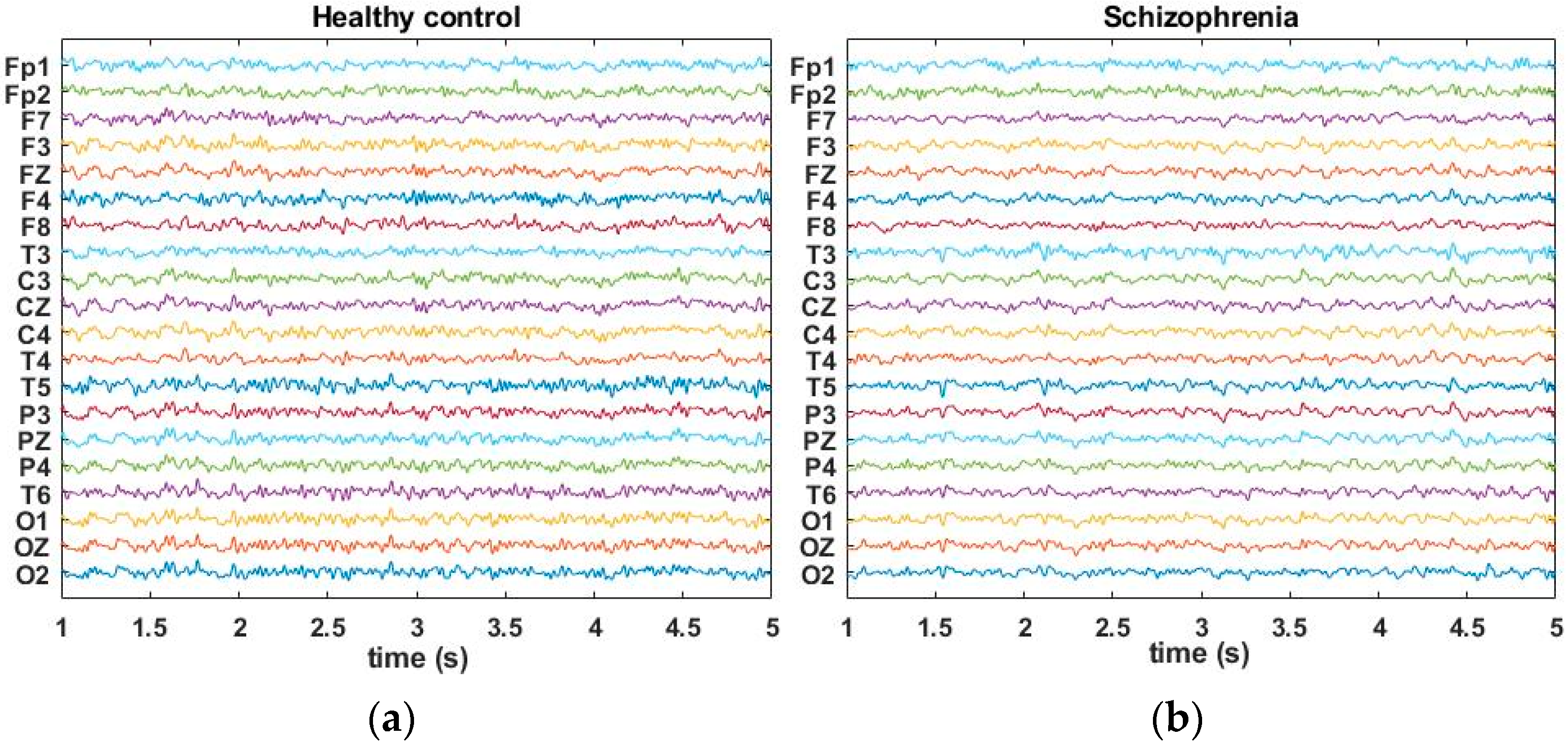
An experienced technician recorded 3.5-min eyes-closed resting-state EEG in a soundproof electromagnetically shielded room using a 10–20 EEG setup with 20 electrodes (Fp1, Fp2, F7, F3, Fz, F4, F8, T3, C3, Cz, C4, T4, T5, P3, Pz, P4, T6, O1, Oz, O2), where the electrodes’ locations follow the unipolar 10–20 Jasper registration scheme [41]. All the recording sessions were scheduled in the morning and the subjects were requested to avoid smoking and consuming coffee, alcohol and drugs before the session. The signals were notch filtered at 60 Hz and band-pass filtered between 0.5 Hz and 80 Hz during the recording and digitalized with the sampling frequency of 204.8 Hz. Figure 1 illustrates an example of EEG recordings for HC and SCZ.
2.3. Data Pre-Processing
To minimize the artifacts, we first band-pass-filtered the EEG signal with cut-off frequencies of 0.5 Hz and 50 Hz. We then used the wavelet-enhanced independent component analysis (wICA) method to detect and remove the components that were contaminated with the artifacts [42]. wICA uses the wavelet threshold to enhance artifact removal with independent components analysis and can therefore better recover the neural activities that are hidden in the artifacts.
2.4. EEG-STE
TE measures the directional information flow between two incidents (data), without assuming any particular model for them, which is especially relevant for detecting the direction of information flow for non-linear interactions with unknown structural information [28,29]. However, estimating the transition probabilities from raw data is not trivial. One solution for this issue is STE. STE transforms the raw data with continuous time series and therefore distribution into symbolic sequences with discretized symbols to simplify the calculation of probability distributions [35]. Here, we briefly describe the STE procedure.
Consider two random processes X = (x1, x2, …, xN) and Y = (y1, y2, …, yN), where xi and yi are the ith samples that are obtained from two regions of the brain. Symbolic transfer entropy (STE) estimates the transfer of information between X and Y with a symbolization process. In this method, first for a given i, m amplitude values Xi = {xi; xi + d; …; xi + (m−1)d} are arranged in an ascending order {xi+(ki1−1)d < xi+(ki2−1)d < … < xi+(kim−1)d}, where m is the embedding dimension, which shows the length of the segments in random processes to be compared, and d is the time delay sample. is then transformed into a sequence of discretized symbols, = {ki1; ki2 …; kim}, where kij, j = 1, 2, … m are the indexes of original elements of . Knowing the two symbol sequences, and , STE is then calculated as [35].
where p denotes the transition probability density, the sum runs over all symbols and t denotes a time step. We used the EEGapp pipeline [43] to calculate the STE between every two electrodes. In this app, firstly, the 3.5-min EEG signal was divided into 21-time segments of 10 s. Then, for each segment, the STE value was computed for a set of d values (d = 1:2:30) and the embedding dimension of m = 3. The maximum value of STE is then selected as the STE between two electrodes, which corresponds to the correct time delay between them. The average of selected STEs among all 21-time segments is then considered as the final STE between two electrodes. This results in 380 STE values for each subject, {STE1,2, STE1,3, STE1,4, ….,STE1,20, STE2,1, STE2,3, …, STE19,20}, where STEi,j measures the directed flow of information from the ith to the jth EEG electrode at each frequency band of (1–4 Hz), (4–8 Hz), (8–13 Hz), (13–30 Hz), and (30–50 Hz). Therefore, the total number of features for all 5 frequency bands is Nc = 380 × 5 = 1900 for each subject.
2.5. Machine Learning
The dataset in this study consists of the STE features for all 132 subjects and their corresponding labels: label 1 for the 62 SCZs and label 2 for the 70 HCs. MLA employs a training set consisting of labeled samples from SCZ and HC subjects to the class of subjects. The most discriminating features, defined as features whose values differ between the SCZ and HC classes, were identified from a list of candidate features, using various types of feature selection algorithms. We need this step to avoid over-fitting, which impacts the classification performance. These selected features then define a feature space. The job of a classifier is to optimally partition the available training samples into two separate regions (i.e., an SCZ region and an HC region) in the feature space. The class of a previously unseen sample can then be determined by extracting the selected features from the sample and plotting the corresponding point in the feature space. The proximity of each subject’s point, in the feature space, to the regions in this feature space occupied by others who are known to be either SCZ or HC, then determines that subject’s class.
In this study, we used the Relief algorithm [44] for selecting the most discriminating feature, which is noise-tolerant and robust to feature interactions. The key idea of the algorithm is to select features according to how their values are similar for the neighboring samples in the same class and different for the neighboring samples in different classes [44]. One repeatedly noted drawback of the Relief algorithm is that it does not effectively remove feature redundancies, i.e., it selects features without considering their correlation. However, unless two features are highly correlated (i.e., redundant), useful information may be lost when redundant features are removed [45,46]. Furthermore, there is an inverse relationship between the correlation of EEG electrodes and their distance. In this study, since we used a low-density EEG set up with just 20 electrodes, the ECs between these electrodes are not highly correlated due to the long distance between them [47].
We used a newly developed consensus nested cross-validation (CN-CV) approach to avoid choosing dominant features among a few subjects [48]. CN-CV is an iterative process, wherein first, the subjects are divided into k (here k = 5) outer folds with the same number of subjects for each class. Then, at each iteration, one particular fold is considered as a test fold and all the features associated with that fold are removed from the training set. The remaining k − 1 folds are then combined and divided into l (here l = 5) inner folds. Then, at each fold l (here l = 1, 2, …, 5), all features with a positive score based on the Relief algorithm, that are more likely to be relevant to classification, are considered as the selected features for that fold. Consensus (common) features through all the l folds are then considered as the feature set for outer fold k. The iterations repeat until all outer folds have been removed from the training set once. The structure of the CN-CV algorithm is analogous to the well-known nested CV(N-CV) [49], but unlike N-CV only feature selection is achieved in each inner fold. This makes the CN-CV algorithm more computationally efficient than the N-CV method that selects fewer irrelevant features [49]. We then selected the first Nr features among all the selected features with the CN-CV approach that gives the highest generalized classification accuracy (averaged accuracy over all k outer folds) as the final selected features.
The third step is to indicate the class (label) of subjects based on the selected features. Various types of classifiers are available for classifying biological signals. In this study, we compare the performance of the five most popular classifiers including Gaussian naïve Bayes (GNB), linear discriminant analysis (LDA), K-nearest neighbors (KNN), support vector machine (SVM), and random forests (RF) using MATLAB R2020a. The choice of these classifiers is based on their effectiveness and simplicity in their implementation. Here, we briefly describe each method.
(1) Gaussian Naïve Bayes (GNB)
GNB method classifies the new data based on applying Bayes’ theorem with the “naive” assumption, where the features are assumed to be independent with Gaussian probability distribution. We used the GNB classifier in our study because of its simplicity and transparency in machine learning modalities [50].
(2) Linear Discriminant Analysis (LDA)
LDA classifier assumes the data samples in each class have Gaussian distribution and the covariance matrices for both classes are the same. As a result, the decision boundary is a linear surface and the LDA predicts the class of a new datum by estimating the probability that it belongs to each class. The class with higher probability is considered the class for the new data. Since the discriminant function is linear, LDA may not be suitable for the non-linearly separable features. Furthermore, this classifier is very sensitive to outliers [51].
(3) K-Nearest Neighbors (KNN)
KNN classifier assigns new data to a specific class if the majority of its k-nearest neighbors belong to that class within the training set. With a sufficiently high value of k and enough training data samples, KNN can produce non-linear decision boundaries. KNN is sensitive to the feature vector dimension [52]. However, it is efficient when the dimension of the feature vector is low [53].
(4) Support Vector Machine (SVM)
SVM classifier creates the hyperplanes known as support vectors that maximize the distance (margin) between the two classes by minimizing the SVM cost function, which leads to maximizing the classification accuracy [54]. SVM is a widely employed classifier in EEG data classification (e.g., [15,16,18,20,24]) because of its high generalization power and relatively good scalability to high-dimensional data.
(5) Random Forests (RF)
RF is an ensemble learning algorithm that combines multiple decision trees at the training stage and uses the mode of their outputs (the class that appears most often) as a final class. This powerful learning algorithm first takes N samples with replacement from the dataset (bootstrapping). It then trains each tree by using a subset of features. Inserting randomness in building RF, makes it robust to the outliers in the database [55]. This method is also widely used for classification based on EEG data (e.g., [21,22]).
In this study, we considered k = 5 neighbors for the KNN classifier, and Gaussian radial basis kernel function and the sequential minimal optimization technique [56] for SVM, and 80 decision trees for RF.
The fourth step is evaluating the classifiers’ performance. Due to the small size of our data sample, we first used the five outer folds of the CN-CV approach in this step to obtain an efficient estimate of classifiers’ performances. Then, to further investigate the performance of the proposed method, we evaluated the classifiers’ performances with another dataset used in studies [19,20,21,22,23] that contains 14 SCZs (7 males (50%), age: 27.9 ± 3.3 and 7 females (50%), age: 28.3 ± 4.1) and 14 HCs (7 males (50%), age: 26.8 ± 2.9 and 7 females (50%), age: 28.7 ± 3.4 years) collected by the Institute of Psychiatry and Neurology in Warsaw, Poland [57], which is available online at RepOD [58].
To evaluate the classifiers’ performance, we measured the sensitivity (SCZ prediction rate or the proportion of SCZs that are correctly identified), specificity (HC prediction rate or the proportion of HCs that are correctly identified), precision (the proportion of subjects classified in SCZ class that are correctly identified), total accuracy (the ratio of the total number of correctly identified SCZs and HCs to the total number of participants), F1-score (a measure of a test’s accuracy that is calculated from the precision and the sensitivity of the test, which is a better metric than the total accuracy to evaluate a classifier when an imbalanced class distribution exists), and the Matthews correlation coefficient (MCC) (a measure of the quality of binary (two-class) classification) for GNB, LDA, SVM, KNN and RF classifiers. These evaluation parameters are represented by
where true positive (TP) is the number of SCZs that are correctly identified, true negative (TN) is the number of HCs that are correctly identified, false positive (FP) is the number of HCs that are misclassified into the SCZ class and false negative (FN) is the number of SCZs that are misclassified into the HC class.
MCC is more reliable than the F1 score and total accuracy in binary classification since it produces a high value only if we have high TP and TN rates and low FP and FN rates [59].
3. Results and Discussion
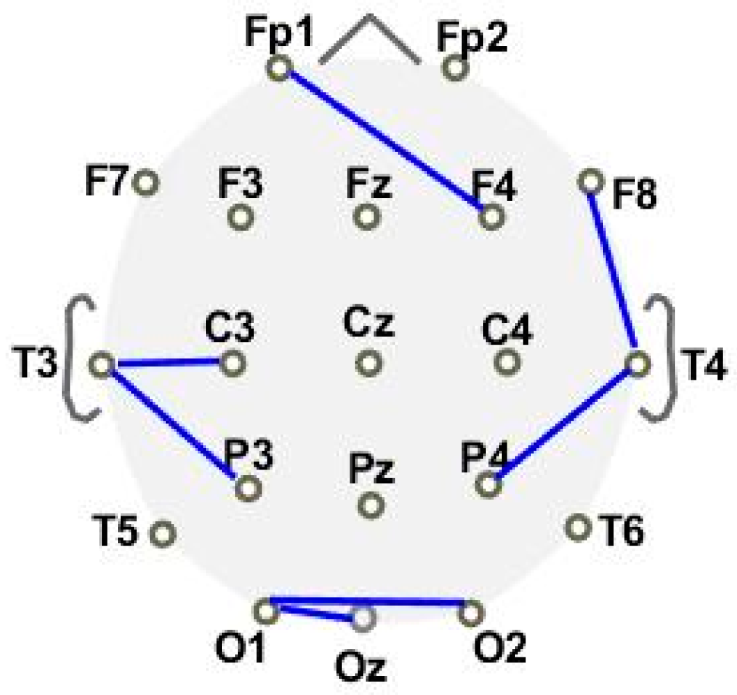
Using the Relief algorithm, Table 2 shows the Nr = 10 most discriminating features between SCZ and HC that provided the highest performance, where the second column of the table indicates the frequency band of the features and the third column shows the areas of the brain that the EC between them using STE is selected as a discriminating feature. For example, from the first row of the table, the first feature is the directed EC from C3 to T3 at frequency band. The illustration of these selected features is shown in Figure 2. The number of features is considerably lower than 106 training samples at each fold that will prevent over-fitting (the feature to the number of training samples ratio is 10/106 × 100 = 9.43%).
From Table 2, four of the selected features are from the connectivity between the occipital areas at different frequency bands (features 4–6, 10). The other features are from left centro–temporal (features 1 and 9), frontal (feature 7), fronto–temporal (feature 8) and parieto–temporal (features 2 and 3), which were also identified in previous studies. Several studies verify a significant alteration in these areas and their connection in SCZs compared to HCs. Here, we briefly describe the outcomes of some of the most recent studies. Tohid et al. [60] conducted a systematic review that reports the results of the relevance of schizophrenia to the occipital lobe. They found out there is enough evidence that supports the concept of a decrease in the volume of the occipital lobe in SCZs. In another study, Maller et al. [61] showed that the prevalence of occipital bending is nearly three times higher among SCZs in comparison to HCs. Kawasaki et al. [62] found a significant decrease in SCZs’ source activities in comparison to HCs, especially in the medial frontal area, superior temporal gyrus, and temporo–parietal junction (TPJ) using the recorded event-related potentials (ERPs) in response to auditory oddball paradigms. Jalili et al. [63] applied a new form of multivariate synchronization analysis called the S-estimator to the high-density resting-state EEG data of SCZs and HCs. They revealed higher synchronization across the left fronto–centro–temporal locations and right fronto–entro–temporo–parietal locations in SCZs than in HCs. Takahashi et al. [64] found that SCZs have a greater complexity than HCs in fronto–centro–temporal regions using multiscale entropy in resting-state EEG activity. Ohi et al. [65] acquired 3T MRI scans from SCZs and HCs. They revealed that SCZs have significantly smaller bilateral superior temporal gyrus volumes than HCs. Pu et al. [66] found significantly smaller hemodynamic changes in SCZs than in HCs in the ventro–lateral prefrontal cortex and the anterior part of the temporal cortex (VLPFC/aTC) and dorso–lateral prefrontal cortex and frontopolar cortex (DLPFC/FPC) regions using 52-channel near-infrared spectroscopy (NIRS). Ibáñez-Molina et al. [67] used the Lempel–Ziv algorithm to assess the complexity of EEG signals in SCZs. They found a higher complexity in the resting-state EEG signals of SCZs at the right frontal area. Using a multivariable TE (MTE), Harmah et al. [68] discovered the brain dysfunction in EC for SCZs in the EEG signals of the oddball task that deteriorated in the parietal and frontal lobes. These two lobes showed more difference between SCZ and HC even during mental activity [15]. Kim et al. [25] showed that the most frequently selected features for classifying the SCZ vs. HC were from the frontal and occipital lobes. Fuentes-Claramontea et al. [69] used the functional MRI (fMRI) scanning of SCZs and HCs while performing a task with three conditions of (1) self-reflection; (2) other reflection; and (3) semantic processing. They showed a connection between alteration in the right TPJ activity and the disorder in self/other differentiation, which could be associated with psychotic symptoms of schizophrenia and affect social functioning in these patients.
Most of the selected features are at and frequency bands. An increase in the first episode and chronic SCZ patients in frequency band is one of the most consistent observations in schizophrenia EEG/ERP studies, which can occur both locally and globally [70]. Furthermore, the EEG signals of SCZ patients show abnormal synchronization in and γ bands, suggesting a crucial role in cognitive deficits and other symptoms of schizophrenia [71].
Table 3 shows the training and test performance for GNB, LDA, SVM, KNN, and RF classifiers that averaged over the five CN-CV outer folds. From Table 3, both the training and test scores are high, ensuring that overfitting has not occurred. Using the test dataset, the KNN classifier can discriminate SCZ from HC with the highest averaged total classification accuracy of 96.92%, followed by the RF, GNB, LDA, and SVM classifiers with total accuracies of 95.47%, 95.44%, 95.44%, and 94.67%, respectively. Comparing the sensitivity and specificity, GNB has the highest sensitivity of 96.67%, followed by RF, KNN, SVM, and LDA with sensitivities of 95.12%, 95%, 91.92%, and 88.59% while KNN has the highest specificity of 98.57%, followed by the SVM, LDA, RF, and GNB with the specificities of 97.14%, 97.14%, 95.71%, and 94.28%, respectively. With regard to precision, KNN has the highest value of 98.33%, followed by SVM, LDA, RF, and GNB with precision values of 96.92%, 96.33%, 95.48%, and 93.81%, respectively. Finally, KNN has the highest F1-score (F1 = 0.97), followed by RF and GNB (F1 = 0.95), SVM (F1 = 0.94), and LDA (F1 = 0.92) and the highest MCC (MCC = 0.94), followed by RF and GNB (MCC = 0.91), SVM (MCC = 0.90), and LDA (MCC = 0.86). These high classification accuracies across different classification algorithms prove that the selected features are highly discriminating between the two classes.
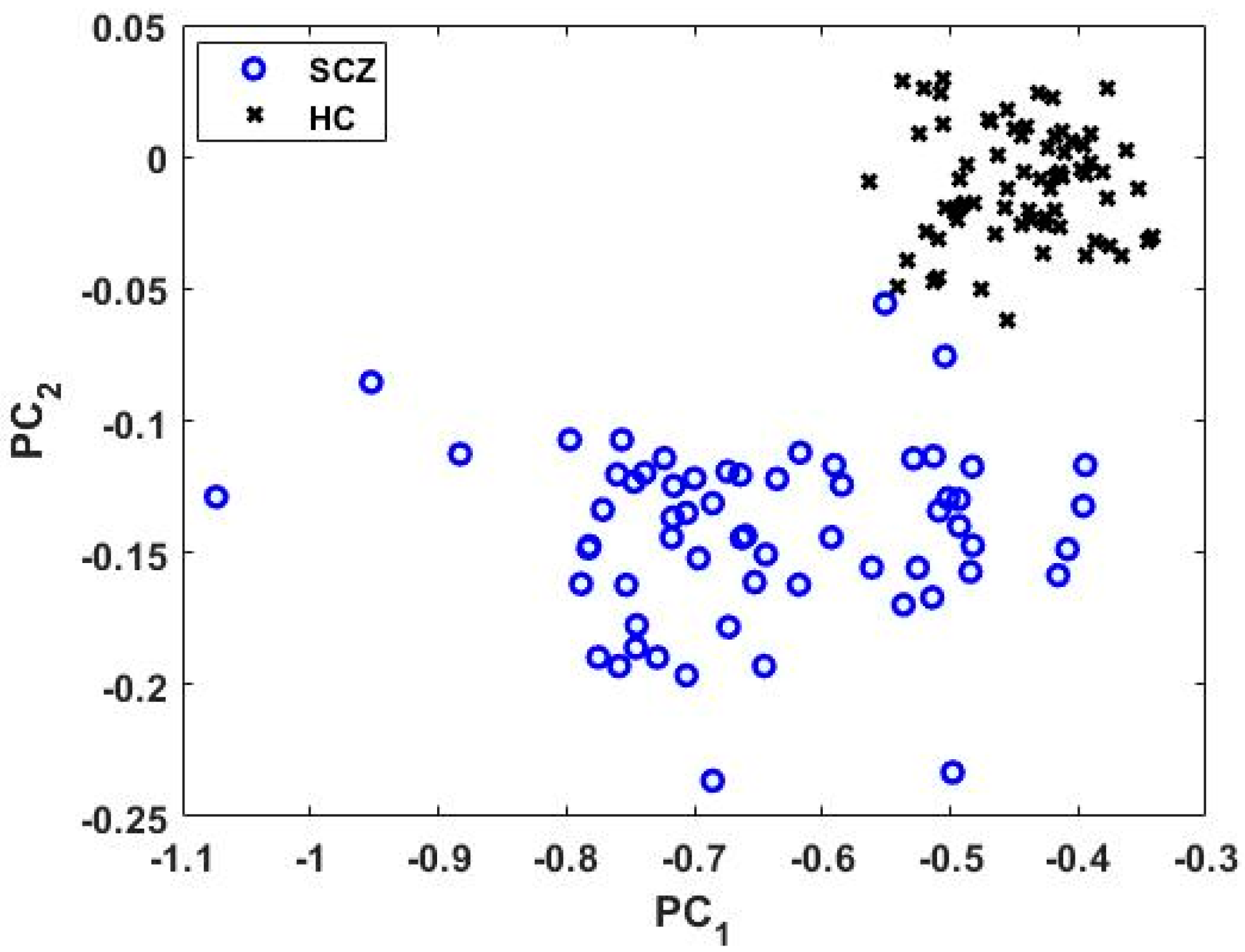
For illustrative purposes, Figure 3 shows a scatter plot of the 62 SCZs (blue circles) and 70 HCs (black crosses), using the kernelized principal component analysis (KPCA) with the polynomial kernel [72]. From the figure, the SCZ and HC clusters are clearly separated, which supports the hypothesis of selecting highly discriminating features. It is worth noting that while the selected features were highly discriminating between the two classes, no correlation was found between the values of the selected features and the symptom severity or duration of illness in SCZ class that showed the selected features were closer to the HC class for patients with less severe symptoms or a shorter duration of illness.
We then evaluated the performance of the classifiers by using the selected features in Table 2 from a new dataset available at RepOD [58]. Table 4 shows the performances of different classifiers discriminating 14 SCZs and 14 HCs from RepOD dataset using 5-fold CN-CV. From Table 4, the performance of all classifiers is above 90%, whereas the highest performance belongs to KNN, SVM, and RF classifiers with the sensitivity of 95.71%, specificity of 100%, precision of 100%, total accuracy of 97.86%, F1-score of 0.98 and MCC of 0.96. This performance is higher than the performance of studies [19,20,21,22], while the new dataset is not used for the feature selection. This proves again that the selected features are very discriminating between SCZ and HC.
4. Conclusions
In this study, we used STE for the first time to develop an MLA to diagnose schizophrenia from resting-state EEG data. Using the relief algorithm, we found a set of 10 discriminating features that differentiated between SCZ and HC. We then first checked the classification performance by using 5-fold CN-CV on our dataset (Table 3) and then on a new dataset available at RepOD [58] (Table 4). From Table 3, the highest accuracy belonged to the KNN classifier (Sensitivity = 95%, specificity = 98.57%, precision = 98.33%, total accuracy = 96.92%, F1-score = 0.97, and MCC = 0.94) and from Table 4, the highest accuracy belonged to KNN, SVM, and RF classifiers (Sensitivity = 95.7%, specificity = 100%, precision = 100%, total accuracy = 97.86%, F1-score = 0.98, and MCC = 0.96).
We note that the performances indicated in Table 3 and Table 4 are higher than typical values obtained from previous studies (Table 1) with a much lower number of features, and less complexity compared to the studies using deep learning approaches. We argue that this performance improvement was due to the effectiveness of the STE method that was employed in the present study. Furthermore, the number of SCZ and HC subjects in this study is higher than most previous studies [11,12,13,14,15,16,17,18,19,20,21,22,23], which can increase the probability of an accurate diagnosis of schizophrenia.
Finally, the selected features are mostly from the EC of occipital, frontal, parieto–temporal, and centro–temporal regions that are in accordance with other research studies related to SCZ. This supports the idea that the proposed MLA can identify features from the regions that are mainly affected by SCZ and that the STE effective connectivity extracted from resting-state EEGs could contribute towards a better understanding of the underlying pathophysiology of schizophrenic illnesses.
While the number of subjects in this study was higher than in most previous studies, it is recommended that the proposed MLA be trained on a bigger dataset with a higher number of SCZ and HC subjects in the future to have a more reliable classification performance. This proposed MLA also has the potential to be used in differentiating between various neuropsychiatric disorders such as major depressive disorder (MDD), bipolar disorder, autism and schizophrenia, as well as predict the response to different treatments available for these diseases. Thus, further work is required to investigate disease-related alterations of EC between brain areas in neuropsychiatric disorders and conditions other than schizophrenia and also the ability to predict the response to different treatments.
Author Contributions
Conceptualization, M.R.; methodology, M.R., C.C., K.M., A.M. and A.D.; software, C.C., K.M., A.M., and A.D.; validation, C.C., K.M., and M.R.; formal analysis, C.C., K.M., and M.R.; investigation, M.R.; resources, M.R.; data curation, M.R.; writing—original draft preparation, M.R. and C.C.; writing—review and editing, M.R. and C.C.; visualization, M.R.; supervision, M.R.; project administration, M.R.; funding acquisition, M.R. All authors have read and agreed to the published version of the manuscript.
Funding
This work was supported by the New York Institute of Technology’s Institutional Support for Research and Creativity (ISRC) Grants.
Institutional Review Board Statement
Ethical review and approval were waived for this study, due to study of existing data where the information is recorded by the investigator in such a manner that the subjects cannot be identified, directly or through identifiers linked to the subjects.
Informed Consent Statement
Informed consent was obtained from all subjects involved in the study.
Data Availability Statement
Not application.
Conflicts of Interest
The authors declare no conflict of interest.
References
- WHO. Available online: https://www.who.int/mental_health/management/schizophrenia/en/ (accessed on 4 October 2019).
- GBD 2017 Disease and Injury Incidence and Prevalence Collaborators. Global, Regional, and National Incidence, Prevalence, and Years Lived with Disability for 354 Diseases and Injuries for 195 Countries and Territories, 1990–2017: A Systematic Analysis for The Global Burden of Disease Study 2017. Lancet 2018, 392, 1789–1858. [Google Scholar] [CrossRef] [Green Version]
- Schmitt, A.; Hasan, A.; Gruber, O.; Falkai, P. Schizophrenia as a disorder of disconnectivity. Eur. Arch. Psychiatry Clin. Neurosci. 2011, 261, S150–S154. [Google Scholar] [CrossRef] [Green Version]
- Pachou, E.; Vourkas, M.; Simos, P.; Smit, D.; Stam, C.J.; Tsirka, V.; Micheloyannis, S. Working Memory in Schizophrenia: An EEG Study Using Power Spectrum and Coherence Analysis to Estimate Cortical Activation and Network Behavior. Brain Topogr. 2008, 21, 128–137. [Google Scholar] [CrossRef]
- Fujimoto, T.; Okumura, E.; Takeuchi, K.; Kodabashi, A.; Otsubo, T.; Nakamura, K.; Kamiya, S.; Higashi, Y.; Yuji, T.; Honda, K.; et al. Dysfunctional Cortical Connectivity During the Auditory Oddball Task in Patients with Schizo-phrenia. Open Neuroimag. J. 2013, 7, 15–26. [Google Scholar] [CrossRef] [PubMed]
- Ravan, M.; Hasey, G.; Reilly, J.P.; MacCrimmon, D.; Khodayari-Rostamabad, A. A Machine Learning Approach Using Audi-tory Odd-ball Responses to Investigate the Effect of Clozapine Therapy. Clin. Neurophysiol. 2015, 126, 721–730. [Google Scholar] [CrossRef] [PubMed]
- Cabral, J.; Kringelbach, M.L.; Deco, G. Exploring the network dynamics underlying brain activity during rest. Prog. Neurobiol. 2014, 114, 102–131. [Google Scholar] [CrossRef] [Green Version]
- Khodayari-Rostamabad, A.; Hasey, G.; MacCrimmon, D.; Reilly, J.P.; de Bruin, H. A Pilot Study to Determine Whether Ma-chine Learning Methodologies Using Pre-Treatment Electroencephalography Can Predict the Symptomatic Response to Clozapine Therapy. Clin. Neurophysiol. 2010, 121, 1998–2006. [Google Scholar] [CrossRef] [PubMed]
- Ravan, M.; Sabesan, S.; D’Cruz, O. On Quantitative Biomarkers of VNS Therapy Using EEG and ECG Signals. IEEE Trans. Biomed. Eng. 2017, 64, 419–428. [Google Scholar] [CrossRef] [PubMed]
- Masychev, K.; Ciprian, C.; Ravan, M.; Manimaran, A.; Deshmukh, A. Quantitative biomarkers to predict response to clozapine treatment using resting EEG data. Schizophr. Res. 2020, 223, 289–296. [Google Scholar] [CrossRef] [PubMed]
- Boostani, R.; Sadatnezhad, K.; Sabeti, M. An efficient classifier to diagnose of schizophrenia based on the EEG signals. Expert Syst. Appl. 2009, 36, 6492–6499. [Google Scholar] [CrossRef]
- Khodayari-Rostamabad, A.; Reilly, J.P.; Hasey, G.M.; de Bruin, H.; MacCrimmon, D.J. Diagnosis of Psychiatric Disorders Us-ing EEG Data and Employing a Statistical Decision Model. In Proceedings of the 2010 Annual International Conference of the IEEE Engineering in Medicine and Biology, Buenos Aires, Argentina, 31 August–4 September 2010. [Google Scholar]
- Sabeti, M.; Katebi, S.; Boostani, R.; Price, G. A new approach for EEG signal classification of schizophrenic and control participants. Expert Syst. Appl. 2011, 38, 2063–2071. [Google Scholar] [CrossRef]
- Langdon, W.B.; Poli, R. Foundations of Genetic Programming; Springer: Berlin/Heidelberg, Germany, 2002. [Google Scholar]
- Thilakvathi, B.; Shenbaga Devi, S.; Bhanu, K.; Malaippan, M. EEG Signal Complexity Analysis for Schizophrenia during Rest and Mental Activity. Biomed. Res. 2017, 28, 1–9. [Google Scholar]
- Liu, H.; Zhang, T.H.; Ye, Y.; Pan, C.; Yang, G.; Wang, J.J.; Qiu, R. A Data Driven Approach for Resting-state EEG signal Clas-sification of Schizophrenia with Control Participants Using Random Matrix Theory. arXiv 2018, arXiv:1712.05289. [Google Scholar]
- Phang, C.R.; Ting, C.M.; Noman, F.; Ombao, H. Classification of EEG-Based Brain Connectivity Networks in Schizophrenia Using a Multi-Domain Connectome Convolutional Neural Network. arXiv 2019, arXiv:1903.08858. [Google Scholar]
- Li, F.; Wang, J.; Liao, Y.; Yi, C.; Jiang, Y.; Si, Y.; Peng, W.; Yao, D.; Zhang, Y.; Dong, W.; et al. Differentiation of Schizophre-nia by Combining the Spatial EEG Brain Network Patterns of Rest and Task P300. IEEE Trans. Neural Syst. Rehabil. Eng. 2019, 27, 594–602. [Google Scholar] [CrossRef]
- Oh, S.L.; Vicnesh, J.; Ciaccio, E.J.; Yuvaraj, R.; Acharya, U.R. Deep Convolutional Neural Network Model for Automated Diagnosis of Schizophrenia Using EEG Signals. Appl. Sci. 2019, 9, 2870. [Google Scholar] [CrossRef] [Green Version]
- Jahmunah, V.; Oh, S.L.; Rajinikanth, V.; Ciaccio, E.J.; Cheong, K.H.; Arunkumar, N.; Rajendra Acharya, U. Automated Detection of Schizophrenia Using Nonlinear Signal Processing Methods. Artif. Intell. Med. 2019, 100, 101698. [Google Scholar] [CrossRef]
- Buettner, R.; Beil, D.; Scholtz, S.; Djemai, A. Development of a Machine Learning Based Algorithm To Accurately Detect Schizophrenia based on One-minute EEG Recordings. In Proceedings of the 53rd Hawaii International Conference on System Sciences, Wailea, HI, USA, 7–10 January 2020. [Google Scholar] [CrossRef] [Green Version]
- Racz, F.S.; Stylianou, O.; Mukli, P.; Eke, A. Multifractal and Entropy-Based Analysis of Delta Band Neural Activity Reveals Altered Functional Connectivity Dynamics in Schizophrenia. Front. Syst. Neurosci. 2020, 14, 49. [Google Scholar] [CrossRef] [PubMed]
- Goshvarpour, A. Schizophrenia diagnosis using innovative EEG feature-level fusion schemes. Phys. Eng. Sci. Med. 2020, 43, 227–238. [Google Scholar] [CrossRef]
- Baradits, M.; Bitter, I.; Czobor, P. Multivariate patterns of EEG microstate parameters and their role in the discrimination of patients with schizophrenia from healthy controls. Psychiatry Res. 2020, 288, 112938. [Google Scholar] [CrossRef] [PubMed]
- Kim, J.-Y.; Lee, H.S.; Lee, S.-H. EEG Source Network for the Diagnosis of Schizophrenia and the Identification of Subtypes Based on Symptom Severity—A Machine Learning Approach. J. Clin. Med. 2020, 9, 3934. [Google Scholar] [CrossRef] [PubMed]
- Koleva, N. When and When Not to Use Deep Learning; Dataiku: New York, NY, USA, 2020. [Google Scholar]
- Friston, K.J. Functional and effective connectivity in neuroimaging: A synthesis. Hum. Brain Mapp. 1994, 2, 56–78. [Google Scholar] [CrossRef]
- Vicente, R.; Wibral, M.; Lindner, M.; Pipa, G. Transfer Entropy-A Model-Free Measure of Effective Connectivity for the Neu-rosciences. J. Comput. Neurosci. 2011, 30, 45–67. [Google Scholar] [CrossRef] [Green Version]
- Faes, L.; Marinazzo, D.; Stramaglia, S. Multiscale Information Decomposition: Exact Computation for Multivariate Gaussian Processes. Entropy 2017, 19, 408. [Google Scholar] [CrossRef] [Green Version]
- Barnett, L.; Barrett, A.B.; Seth, A.K. Granger Causality and Transfer Entropy Are Equivalent for Gaussian Variables. Phys. Rev. Lett. 2009, 103, 238701. [Google Scholar] [CrossRef] [Green Version]
- Antonacci, Y.; Astolfi, L.; Nollo, G.; Faes, L. Information Transfer in Linear Multivariate Processes Assessed through Penalized Regression Techniques: Validation and Application to Physiological Networks. Entropy 2020, 22, 732. [Google Scholar] [CrossRef]
- Kaiser, A.; Schreiber, T. Information Transfer in Continuous Processes Physica D: Nonlin. Phenomena 2002, 166, 43–62. [Google Scholar]
- Verdes, P.F. Assessing causality from multivariate time series. Phys. Rev. E Stat. Nonlin. Bio. Soft Matter Phys. 2005, 72, 026222. [Google Scholar] [CrossRef]
- Lungarella, M.; Pitti, A.; Kuniyoshi, Y. Information transfer at multiple scales. Phys. Rev. E Stat. Nonlin. Bio. Soft Matter Phys. 2007, 76, 056117. [Google Scholar] [CrossRef] [Green Version]
- Staniek, M.; Lehnertz, K. Symbolic Transfer Entropy. Phys. Rev. Lett. 2008, 100, 158101. [Google Scholar] [CrossRef]
- Jordan, D.; Ilg, R.; Schneider, G.; Stockmanns, G.; Kochs, E.F. EEG Measures Indicating Anesthesia Induced Changes of Cortical Information Processing. Biomed. Tech. 2013, 58 (Suppl. 1G), 139–140. [Google Scholar]
- Lehnertz, K.; Dickten, H. Assessing directionality and strength of coupling through symbolic analysis: An application to epilepsy patients. Philos. Trans. R. Soc. A: Math. Phys. Eng. Sci. 2015, 373, 20140094. [Google Scholar] [CrossRef]
- Zhou, G.; Pan, Y.; Yang, J.; Zhang, X.; Guo, X.; Luo, Y. Sleep Electroencephalographic Response to Respiratory Events in Pa-tients with Moderate Sleep Apnea–Hypopnea Syndrome. Front. Neurosci. 2020, 14, 310. [Google Scholar] [CrossRef]
- Ciprian, C.; Masychev, K.; Ravan, M.; Manimaran, A.; Deshmukh, A. A Machine Learning Approach Using Effective Con-nectivity to Predict Response to Clozapine Treatment. IEEE Trans. Neural. Syst. Rehabil. Eng. 2020, 28, 2598–2607. [Google Scholar] [CrossRef] [PubMed]
- Diagnostic and Statistical Manual of Mental Disorders: DSM-IV, 4th ed.; American Psychiatric Association: Washington, DC, USA, 1994.
- Jasper, H.H. The Ten-Twenty Electrode System of the International Federation. EEG Clin. Neurophysiol. 1958, 10, 371–375. [Google Scholar]
- Castellanos, N.P.; Makarov, V.A. Recovering EEG brain signals: Artifact suppression with wavelet enhanced independent component analysis. J. Neurosci. Methods 2006, 158, 300–312. [Google Scholar] [CrossRef]
- EEGapp, BIAPT lab, McGill University. Available online: https://github.com/BIAPT/EEGapp/wiki (accessed on 23 December 2017).
- Liu, H.; Motoda, H. Computational Methods of Feature Selection, 1st ed.; Chapman & Hall: Boca Raton, FL, USA, 2008. [Google Scholar]
- Elisseeff, G.A. An Introduction to Variable and Feature Selection. J. Mach. Learn. Res. 2003, 3, 1157–1182. [Google Scholar]
- Urbanowicz, R.J.; Meeker, M.; La Cava, W.; Olson, R.S.; Moore, J.H. Relief-based feature selection: Introduction and review. J. Biomed. Inform. 2018, 85, 189–203. [Google Scholar] [CrossRef] [PubMed]
- Bhavsar, R.; Sun, Y.; Helian, N.; Davey, N.; Mayor, D.; Steffert, T. The Correlation between EEG Signals as Measured in Different Positions on Scalp Varying with Distance. Procedia Comput. Sci. 2018, 123, 92–97. [Google Scholar] [CrossRef]
- Parvandeh, S.; Yeh, H.-W.; Paulus, M.P.; McKinney, B.A. Consensus features nested cross-validation. Bioinformatics 2020, 36, 3093–3098. [Google Scholar] [CrossRef] [PubMed]
- Gavin, C.C.; Talbot, N.L.C. On Over-Fitting in Model Selection and Subsequent Selection Bias in Performance Evaluation. J. Mach. Learn. Res. 2017, 11, 2079–2107. [Google Scholar]
- Brownlee, J. Master Machine Learning Algorithms: Discover How They Work and Implement Them from Scratch; Machine Learning Mastery: Melbourne, VIC, Australia, 2016. [Google Scholar]
- Bashashati, H.; Ward, R.K.; Birch, G.E.; Bashashati, A. Comparing Different Classifiers in Sensory Motor Brain Computer Interfaces. PLoS ONE 2015, 10, e0129435. [Google Scholar] [CrossRef] [PubMed]
- Friedman, J.H.K. On Bias, Variance, 0/1-Loss, and the Curse-of-Dimensionality. Data Min. Knowl. Discov. 1997, 1, 55–77. [Google Scholar] [CrossRef]
- Borisoff, J.F.; Mason, S.G.; Bashashati, A.; Birch, G.E. Brain–Computer Interface Design for Asynchronous Control Applications: Improvements to the LF-ASD Asynchronous Brain Switch. IEEE Trans. Biomed. Eng. 2004, 51, 985–992. [Google Scholar] [CrossRef] [PubMed]
- Hsu, C.W.; Chang, C.C.; Lin, C.J. A Practical Guide to Support Vector Classification; Department of Computer Science, National Taiwan University: Taipei, Taiwan, 2003. [Google Scholar]
- Criminisi, A.; Shotton, J. Decision Forests for Classification, Regression, Density Estimation, Manifold Learning and Semi-Supervised Learning; Microsoft Research Ltd.: Cambridge, UK, 2012. [Google Scholar]
- Platt, J. Sequential Minimal Optimization: A Fast Algorithm for Training Support Vector Machines; MSR-TR-98-14; Microsoft Research Ltd.: Cambridge, UK, 1988. [Google Scholar]
- Olejarczyk, E.; Jernajczyk, W. Graph-based analysis of brain connectivity in schizophrenia. PLoS ONE 2017, 12, e0188629. [Google Scholar] [CrossRef] [PubMed]
- Olejarczyk, E.; Jernajczyk, W. EEG in schizophrenia. RepOD 2017. [Google Scholar] [CrossRef]
- Chicco, D.; Jurman, G. The advantages of the Matthews correlation coefficient (MCC) over F1 score and accuracy in binary classification evaluation. BMC Genom. 2020, 21, 1–13. [Google Scholar] [CrossRef] [Green Version]
- Tohid, H.; Faizan, M.; Faizan, U. Alterations of the occipital lobe in schizophrenia. Neurosciences 2015, 20, 213–224. [Google Scholar] [CrossRef] [PubMed] [Green Version]
- Maller, J.J.; Anderson, R.J.; Thomson, R.H.; Daskalakis, Z.J.; Rosenfeld, J.V.; Fitzgerald, P.B. Occipital Bending in Schizophrenia. Aust. N. Z. J. Psychiatry 2017, 51, 32–41. [Google Scholar] [CrossRef] [PubMed] [Green Version]
- Kawasaki, Y.; Sumiyoshi, T.; Higuchi, Y.; Ito, T.; Takeuchi, M.; Kurachi, M. Voxel-based analysis of P300 electrophysiological topography associated with positive and negative symptoms of schizophrenia. Schizophr. Res. 2007, 94, 164–171. [Google Scholar] [CrossRef] [PubMed]
- Jalili, M.; Lavoie, S.; Deppen, P.; Meuli, R.; Do, K.Q.; Cuénod, M.; Hasler, M.; Feo, O.D.; Knyazeva, M.G. Dysconnection To-pography in Schizophrenia Revealed with State-Space Analysis of EEG. PLoS ONE 2007, 2, e1059. [Google Scholar] [CrossRef] [Green Version]
- Takahashi, T.; Cho, R.Y.; Mizuno, T.; Kikuchi, M.; Murata, T.; Takahashi, K.; Wada, Y. Antipsychotics reverse abnormal EEG complexity in drug-naive schizophrenia: A multiscale entropy analysis. NeuroImage 2010, 51, 173–182. [Google Scholar] [CrossRef] [Green Version]
- Ohi, K.; Matsuda, Y.; Shimada, T.; Yasuyama, T.; Oshima, K.; Sawai, K.; Kihara, H.; Nitta, Y.; Okubo, H.; Uehara, T.; et al. Structural alterations of the superior temporal gyrus in schizophrenia. Eur. Psychiatry 2016, 35, 25–31. [Google Scholar] [CrossRef] [PubMed]
- Pu, S.; Nakagome, K.; Itakura, M.; Iwata, M.; Nagata, I.; Kaneko, K. Association of fronto-temporal function with cognitive ability in schizophrenia. Sci. Rep. 2017, 7, 42858. [Google Scholar] [CrossRef] [PubMed] [Green Version]
- Ibáñez-Molina, A.J.; Lozano, V.; Soriano, M.F.; Aznarte, J.I.; Gómez-Ariza, C.J.; Bajo, M.T. EEG Multiscale Complexity in Schizophrenia During Picture Naming. Front. Physiol. 2018, 9, 1213. [Google Scholar] [CrossRef] [Green Version]
- Harmah, D.J.; Li, C.; Li, F.; Liao, Y.; Wang, J.; Ayedh, W.M.A.; Bore, J.C.; Yao, D.; Dong, W.; Xu, P. Measuring the Non-linear Directed Information Flow in Schizophrenia by Multivariate Transfer Entropy. Front. Comput. Neurosci. 2020, 13. [Google Scholar] [CrossRef]
- Fuentes-Claramontea, P.; Martin-Suberoa, M.; Salgado-Pinedaa, P.; Santo-Anglesa, A.; Argila-Plazaa, I.; Salavertc, J.; Arévaloe, A.; Bosquef, C.; Sarrif, C.; Guerrero-Pedrazaf, A.; et al. Brain imaging correlates of self- and other-reflection in schizophrenia. Neuroimage Clin. 2020, 25, 102134. [Google Scholar] [CrossRef] [PubMed]
- Sponheim, S.R.; Clementz, B.A.; Iacono, W.G.; Beiser, M. Resting EEG in first-episode and chronic schizophrenia. Psychophysiol. 1994, 31, 37–43. [Google Scholar] [CrossRef]
- Uhlhaas, P.J.; Singer, W. Abnormal neural oscillations and synchrony in schizophrenia. Nat. Rev. Neurosci. 2010, 11, 100–113. [Google Scholar] [CrossRef] [PubMed]
- Muller, K.-R.; Mika, S.; Ratsch, G.; Tsuda, K.; Schoelkopf, B. An introduction to kernel-based learning algorithms. IEEE Trans. Neural Netw. 2001, 12, 181–201. [Google Scholar] [CrossRef] [PubMed] [Green Version]
Figure 1.
EEg signals of (a) a healthy control and (b) a schizophrenic patient.

Figure 2.
A rough schematic drawing which shows the selected features by connections (solid thick blue lines).
Figure 2.
A rough schematic drawing which shows the selected features by connections (solid thick blue lines).

Figure 3.
Scatter plot of the feature space showing SCZ (blue circles) vs. HC (black crosses).


Table 1.
Summary of most recent and accurate automated frameworks to diagnose schizophrenia using resting-state EEG data.
Table 1.
Summary of most recent and accurate automated frameworks to diagnose schizophrenia using resting-state EEG data.
| Article | # of Features | Classifier | Best Accuracy | EEG Dataset |
|---|---|---|---|---|
| Boostani et al. (2009) [11] | 286 | BDLDA | 87.51% | 13 SCZs and 18 HCs |
| Khodayari et al. (2010) [12] | 42 | MFA | 87.1% | 40 SCZs, 64 MDDs, and 91 HCs |
| Sabeti et al. (2011) [13] | 80 | Adaboost | 91.94% | 20 SCZs and 20 HCs |
| Thilakvathi et al. (2017) [15] | 10 | SVM | 80% | 55 SCZs and 23 HCs |
| Liu et al. (2018) [16] | 1500 | SVM | 91.16% | 40 SCZs and 40 HCs |
| Phang et al. (2019) [17] | 2730 | MDC-CNN | 93.06% | 45 SCZs and 39 HCs |
| Li et al. (2019) [18] | 4 | SVM | 88.10% | 19 SCZs and 23 HCs |
| Oh et al. (2019) [19] | - | CNN | 81.26% | 14 SCZs and 14 HCs |
| Jahmunah et al. (2019) [20] | 14 | SVM | 92.91% | 14 SCZs and 14 HCs |
| Buettner et al. (2020) [21] | 200 | RF | 96.77% | 14 SCZs and 14 HCs |
| Racz et al. (2020) [22] | 21 | RF | 89.29% | 14 SCZ and 14 HCs |
| Goshvarpour et al. (2020) [23] | 19 | PNN | 100% | 14 SCZs and 14 HCs |
| Baradits et al. (2020) [24] | 14 | SVM | 82.7% | 70 SCZs and 75 HCs |
| Kim et al. (2020) [25] | 27 | LDA | 80.66% | 119 SCZs and 119 HCs |
Table 2.
The 10 discriminating features between SCZ and HC groups.
| Feature # | Frequency Band | Effective Connectivity Feature |
|---|---|---|
| 1 | C3 to T3 | |
| 2 | P3 to T3 | |
| 3 | P4 to T4 | |
| 4 | O1 to Oz | |
| 5 | O1 to O2 | |
| 6 | O1 to O2 | |
| 7 | Fp1 to F4 | |
| 8 | F8 to T4 | |
| 9 | C3 to T3 | |
| 10 | O1 to O2 |
Table 3.
Classification performance of different classifiers discriminating 62 SCZ from 70 HC subjects using 5-fold CN-CV.
Table 3.
Classification performance of different classifiers discriminating 62 SCZ from 70 HC subjects using 5-fold CN-CV.
| Classifier | Sensitivity | Specificity | Precision | Total Accuracy | F1-Score | MCC | |
|---|---|---|---|---|---|---|---|
| Training Performance | GNB | 97.97% | 95.71% | 95.33% | 96.78% | 0.97 | 0.94 |
| LDA | 91.53% | 99.29% | 99.12% | 96.78% | 0.95 | 0.91 | |
| SVM | 98.38% | 98.93% | 98.82% | 98.68% | 0.99 | 0.97 | |
| KNN | 95.56% | 98.57% | 98.33% | 97.15% | 0.97 | 0.94 | |
| RF | 100% | 100% | 100% | 100% | 1 | 1 | |
| Test Performance | GNB | 96.67% | 94.28% | 93.81% | 95.44% | 0.95 | 0.91 |
| LDA | 88.59% | 97.14% | 96.33% | 95.44% | 0.92 | 0.86 | |
| SVM | 91.92% | 97.14% | 96.92% | 94.67% | 0.94 | 0.90 | |
| KNN | 95.00% | 98.57% | 98.33% | 96.92% | 0.97 | 0.94 | |
| RF | 95.12% | 95.71% | 95.48% | 95.47% | 0.95 | 0.91 |
MCC: Matthews correlation coefficient.
Table 4.
Classification performance of different classifiers discriminating 14 SCZ from 14 HC subjects from dataset available at RepOD [58] using 5-fold CN-CV.
Table 4.
Classification performance of different classifiers discriminating 14 SCZ from 14 HC subjects from dataset available at RepOD [58] using 5-fold CN-CV.
| Classifier | Sensitivity | Specificity | Precision | Total Accuracy | F1-Score | MCC |
|---|---|---|---|---|---|---|
| GNB | 90% | 91.43% | 91.32% | 90.71% | 0.90 | 0.81 |
| LDA | 90% | 91.43% | 91.32% | 90.71% | 0.90 | 0.81 |
| SVM | 95.71% | 100% | 100% | 97.86% | 0.98 | 0.96 |
| KNN | 95.71% | 100% | 100% | 97.86% | 0.98 | 0.96 |
| RF | 95.71% | 100% | 100% | 97.86% | 0.98 | 0.96 |
MCC: Matthews correlation coefficient.
Publisher’s Note: MDPI stays neutral with regard to jurisdictional claims in published maps and institutional affiliations. |
© 2021 by the authors. Licensee MDPI, Basel, Switzerland. This article is an open access article distributed under the terms and conditions of the Creative Commons Attribution (CC BY) license (https://creativecommons.org/licenses/by/4.0/).
Share and Cite
MDPI and ACS Style
Ciprian, C.; Masychev, K.; Ravan, M.; Manimaran, A.; Deshmukh, A. Diagnosing Schizophrenia Using Effective Connectivity of Resting-State EEG Data. Algorithms 2021, 14, 139. https://0-doi-org.brum.beds.ac.uk/10.3390/a14050139
AMA Style
Ciprian C, Masychev K, Ravan M, Manimaran A, Deshmukh A. Diagnosing Schizophrenia Using Effective Connectivity of Resting-State EEG Data. Algorithms. 2021; 14(5):139. https://0-doi-org.brum.beds.ac.uk/10.3390/a14050139
Chicago/Turabian StyleCiprian, Claudio, Kirill Masychev, Maryam Ravan, Akshaya Manimaran, and AnkitaAmol Deshmukh. 2021. "Diagnosing Schizophrenia Using Effective Connectivity of Resting-State EEG Data" Algorithms 14, no. 5: 139. https://0-doi-org.brum.beds.ac.uk/10.3390/a14050139
Note that from the first issue of 2016, this journal uses article numbers instead of page numbers. See further details here.