Article

Accelerating In-Transit Co-Processing for Scientific Simulations Using Region-Based Data-Driven Analysis

1
Graduate School of Information Science and Technology, Osaka University, Suita-shi 565-0871, Japan
2
University of Nicosia, Nicosia CY-2417, Cyprus
3
Department of Mechanical and Aerospace Engineering, University of Strathclyde, Glasgow G1 1XJ, UK
*
Author to whom correspondence should be addressed.
Submission received: 14 April 2021 / Revised: 10 May 2021 / Accepted: 10 May 2021 / Published: 12 May 2021
(This article belongs to the Collection Parallel and Distributed Computing: Algorithms and Applications)

Abstract

:
Increasing processing capabilities and input/output constraints of supercomputers have increased the use of co-processing approaches, i.e., visualizing and analyzing data sets of simulations on the fly. We present a method that evaluates the importance of different regions of simulation data and a data-driven approach that uses the proposed method to accelerate in-transit co-processing of large-scale simulations. We use the importance metrics to simultaneously employ multiple compression methods on different data regions to accelerate the in-transit co-processing. Our approach strives to adaptively compress data on the fly and uses load balancing to counteract memory imbalances. We demonstrate the method’s efficiency through a fluid mechanics application, a Richtmyer–Meshkov instability simulation, showing how to accelerate the in-transit co-processing of simulations. The results show that the proposed method expeditiously can identify regions of interest, even when using multiple metrics. Our approach achieved a speedup of 1.29 × in a lossless scenario. The data decompression time was sped up by 2 × compared to using a single compression method uniformly.

1. Introduction

The processing capabilities of modern supercomputers are improving at a tremendous pace. However, input/output (I/O) bandwidth has advanced at a much slower rate, leading to bottlenecks in many applications [1,2]. This is one of the most pressing matters for large-scale scientific simulations. Simulations can result in multiple tera- or petabytes of generated data, making it challenging to save all necessary data to permanent storage due to limited storage capacity or time-consuming I/O operations [3,4,5,6]. In-situ or in-transit visualization and analysis are often used for each time step while the data is generated.
In-situ co-processing is typically performed on the same compute nodes as the simulation and can achieve high performance, partly because of the locality of the data. However, in-situ co-processing takes up valuable simulation time. Many researchers are reluctant to dedicate computing resources used by the simulation to other compute-intensive tasks [2,4], meaning that the time available for in-situ co-processing often is short compared to that of the simulation. One option to reduce the co-processing time is to lower the frequency at which time steps are analyzed. Another is to limit the available time to perform co-processing for each analyzed time step. Both these options are undesirable because they limit the amount of data available to the researcher after the simulation has been completed. Furthermore, a significant amount of the available memory is used by the simulation in an in-situ scenario, meaning that only a tiny amount can be allocated for visualization or analysis purposes [7].
In contrast, in-transit co-processing [8,9], illustrated in Figure 1, is generally performed on a separate group of compute nodes, which we refer to as transit nodes. Utilizing a different group of nodes means that co-processing can be performed asynchronously during the simulation stage, resulting in a less strict time limitation than an in-situ approach. Furthermore, the transit nodes can be equipped with different hardware to accelerate the co-processing tasks. The main drawback of in-transit co-processing is that the relevant simulation data needs to be transferred to the transit nodes. Moreover, it is not guaranteed that the simulation nodes can hold an extra copy of the data in memory. It is often impossible to transfer the data asynchronously while simulating the next time step.
The data transfer required to perform in-transit co-processing can be accelerated by reducing or compressing the simulation data. However, using a reduction or a lossy compression method could lower the detail and accuracy of the whole data set, including regions of interest. It could instead be beneficial to selectively compress areas of data based on their contribution to the simulated phenomenon. Reducing or compressing areas that are not of interest would result in less time-consuming data transfers without any significant loss in the data quality.
To determine the frequency at which data is analyzed, the time available for co-processing and what compression method(s) to use to accelerate the data transfers, there is a need to identify the importance of the underlying simulation data. Such information can be used for a wide variety of cases, including guiding the simulation, determining which time steps of the simulation to analyze or save to permanent storage, removing or reducing unimportant data, and finding interesting camera locations for co-processing purposes. Some of these cases have been explored in related work [10,11,12,13,14,15,16,17]. However, these methods have either been limited in the amount of used importance metrics [10,12,13,14,15,16,17] or been unable to combine multiple metrics to create advanced importance metrics and to make more advanced decisions [11].
We propose a method that efficiently can identify the importance of subsets of simulation data, which consists of multivariate and temporal data sets in the form of structured rectilinear grids. User-defined importance metrics and filters are used to determine the importance of blocks; contiguous and convex regions of data that combined make up the generated simulation data. The calculated importance can then be used for a wide variety of purposes to accelerate or guide the simulation, such as identifying important regions, down-sample, reducing, compressing, or simply removing parts of the data based on user-defined constraints and the underlying hardware. What sets the proposed method apart from related work is its ability to calculate importance when using multiple analyses efficiently. It can adaptively make any number of decisions based on the importance, compared to only a binary decision, which is typical in other methods.
We also propose an approach that uses the proposed method to identify how to best combine the usage of multiple different compression methods based on the importance of the underlying data, which can be seen as a use case of the proposed method. In the case of lossy compression, loss of detail in regions of interest can be kept at a minimum by reducing unimportant areas. Using this data-driven approach, we strive to reduce the data size and the in-transit data transfer time to accelerate in-transit co-processing. The main contributions of this work are as follows:
  • An efficient method to determine the block importance of large-scale simulations. Calculating the importance of various regions of data was a time-consuming task in many related works. As such, only a few importance metrics tend to be used. The main goal of our proposed method is to provide researchers with a customizable and easy-to-use way to efficiently determine the importance of subsets of large-scale simulation data, even when using multiple complex analyses to determine such importance. To reach this goal, we have developed a scheme that uses a separate buffer to transform the data to a more suitable structure for analysis and strives to schedule importance analyses in a fashion that improves the cache hit rates. We also introduce the usage of an adaptive condition window; a custom range within which multiple condition parameters can vary. Using a condition window allows parameters to change based on the current constraints of the environment. For example, if a data transfer is too time-consuming, the parameters can be adapted to compress or remove more data in the coming time step.
  • A flexible approach to accelerate in-transit co-processing. We observe that the effectiveness of a certain compression algorithm often depends on the underlying compressed data. By identifying the importance and the most suitable compression for each region of generated simulation data, we strive to minimize the data size and the in-transit data transfer time by combining the use of multiple compression methods integrated into a pipeline. The approach explored in this paper puts no additional restraints on the contents of the co-processing stage. It can be used in tandem with various visualization software, e.g., Paraview [18], VisIt [19], or OSPRay [20].
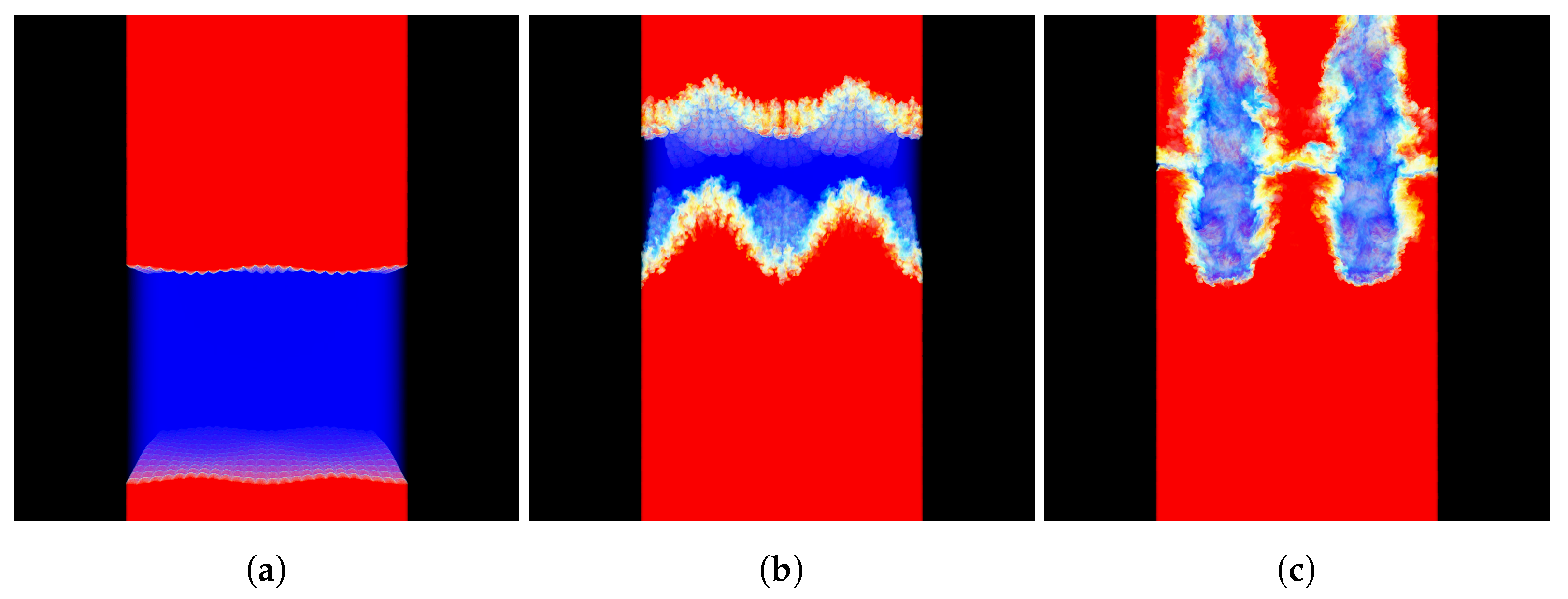
  • A case study of how the in-transit co-processing of a Richtmyer–Meshkov instability (RMI) simulation can be accelerated using the proposed approach. The RMI simulation is performed using CNS3D, a state-of-the-art program for numerical fluid simulations.
The structure of this paper is organized as follows. Related work is discussed in Section 2. The proposed approach is presented in Section 3. In Section 4, we evaluate the performance of the proposed approach. Lastly, our conclusions are presented in Section 5.

2. Related Work

Determining and analyzing regions of interest in three-dimensional (3D) data sets has been an important topic in many research fields, and has as such been explored in many related works [10,11,12,13,14,15,16,17]. A commonly used technique is Adaptive Mesh Refinement (AMR) [13,14,15]. Using AMR, the simulated region is divided into multiple sub-regions, commonly by using a tree structure such as an octree [21]. After the simulation has been completed, important regions in the tree structure are subdivided to create even smaller sub-regions, on which more compute-intensive operations can be used to, for example, increase the accuracy or resolution of the simulation. This process can be performed recursively based on the researcher’s specifications. The analysis required to calculate block-based importance metrics results in a fairly uniform data access over all data points in the simulation region. As such, the recursive, top-down AMR approach could result in redundant calculations and low cache hit rates. This notion is confirmed in related work [12], where a bottom-up approach, i.e., calculating the importance of each individual block, could achieve significantly better performance.
Close to our work is a paper by Dorier et al. [10], in which calculated importance metrics were used to adaptively reduce unimportant blocks. The technique targets explicitly in-situ visualization and supports elementary data reduction and load balancing based on a random distribution. However, the technique only supports a single reduction strategy. Furthermore, their technique assumes that simulation data is stored as blocks, which is not the case for most simulations. For their technique to work in the general case, all simulation data first needs to be preprocessed and partitioned into blocks, which is time-consuming and increases the memory usage as two sets of the simulation data need to be maintained while performing the importance analysis.
Wang et al. [11] introduced an importance curve to store the derived importance of all data blocks for a time-varying data set. By analyzing the changing block importance between different time steps it would be possible to characterize temporal behaviors exhibited by simulation data. Such information could be used to make informed processing decisions, e.g., setting a time budget for the co-processing stage or saving data to permanent storage.
Nouanesengsy et al. [12] presented a prioritization method for 3D data sets inspired by AMR. Data sets were recursively partitioned into smaller regions based on user defined importance metrics. A prioritization tree was constructed for the data set, which then could be used to identify interesting camera placements or to determine compression strategies for saving data to permanent storage.
Some data sampling and summarization methods [16,17] use importance based on entropy metrics to prioritize the reduction of unimportant data. Here, reduced subsets of the simulation data are saved to permanent storage for post-hoc analysis; more than 99 % of simulation data is removed in some applications [16]. Data sampling methods are not suited for applications that operate on lossless simulation data. Moreover, these methods do not support use cases that require custom metrics to define important data.
Table 1 shows a qualitative comparison to related work. Here, we specifically compare features related to the use case considered in this work. Method [11] is processed post-hoc, whereas methods [12,13,14,15] have no defined behavior of how to use the calculated importance values to compress unimportant data. Out of the methods used for comparison, only related work [10,16,17] explore using the data importance to prioritize compression or reduction of unimportant data. However, in contrast to our work, none of the methods support lossless compression or simultaneously using multiple compression and reduction methods. In addition, there is no defined behavior of how to use the methods for in-transit co-processing. A quantitative comparison is difficult, as each work has a different feature set and use case. We, therefore, chose to evaluate our method independently, as was also done in related work [10,11,12].
Many visualization and analysis techniques have been proposed for in-situ and in-transit co-processing. Some aim to batch-render images of each time step of the simulation from multiple viewpoints, thus allowing researchers to interactively explore different regions of the simulation post-hoc [22,23]. Other techniques focus on extracting features, metadata, or samples of the simulation [2,24,25,26]. Using many different types of visualizations and analyses would generally be desired to extract as much information from the simulation as possible. However, each additional task would increase the execution time. The logical approach would be to use in-transit co-processing in such a scenario due to the often limited time available to perform such computations in-situ. To make in-transit co-processing a viable option, we need new techniques to achieve faster data transfers between simulation and transit nodes. Many researchers have developed methods to lower the data transfer time required to perform in-transit co-processing [5,27,28,29]. Most works have focused on uniformly reducing or compressing data [5,27,28]. Although efficient, regions of interest within the data are reduced to the same extent as unimportant regions.
Lossy compression methods such as zfp [30] and an extension of SZ [31] strive to lower the compression error by analyzing the entropy of the data. Data sets are split into blocks of size 4 × 4 × 4 and 6 × 6 × 6 , respectively. A function is then used to predict a suitable level of compression for each block, based on the estimated compression error. These lossy methods have proved to achieve good performance [30,31]. However, the fact that they are lossy makes them unusable in many use cases. We also note that these methods are unable to determine the importance of regions of data, and that although the level of compression varies, they ultimately use the same lossy compression method on the whole data set. Both of these compression methods can be integrated into the proposed approach, as presented in Section 3, to be used on a subset of the available data blocks.
In summary, effectively performing in-transit co-processing of data generated by scientific simulations remains an important research topic in the field of high-performance computing. Many methods which uniformly reduce or compress data have been proposed. However, the characteristics of the simulation data can vary substantially depending on the current time step, meaning that the need for compression and analysis also can vary. Some techniques which analyze the characteristics of the data also exist. However, one of the most commonly used techniques, AMR, is often unable to efficiently calculate individual block importance because of the different data access pattern. Although alternatives [10,11,12,16,17] have been proposed, they are generally limited in scope or in their ability to perform multiple analyses to determine block importance or characteristics of different parts in the studied simulation data. Our work improves upon this related work by efficiently handling multiple importance analyses and by adaptively utilizing multiple different compression and reduction strategies.

3. Adaptive In-Transit Co-Processing

In this section, we present the proposed method and an approach to accelerate in-transit co-processing. To the best of our knowledge, this is the first work to accelerate in-transit processing by simultaneously using more than one compression method based on multiple importance analyses of the underlying simulation data. The workflow of the approach is shown in Figure 2.
The approach consists of three distinct stages:
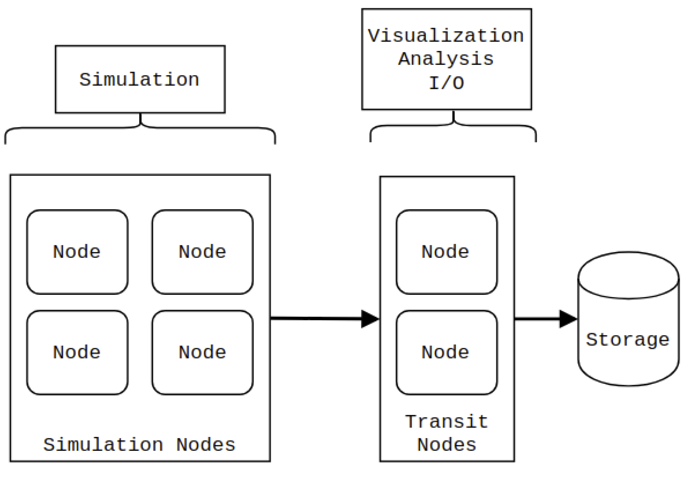
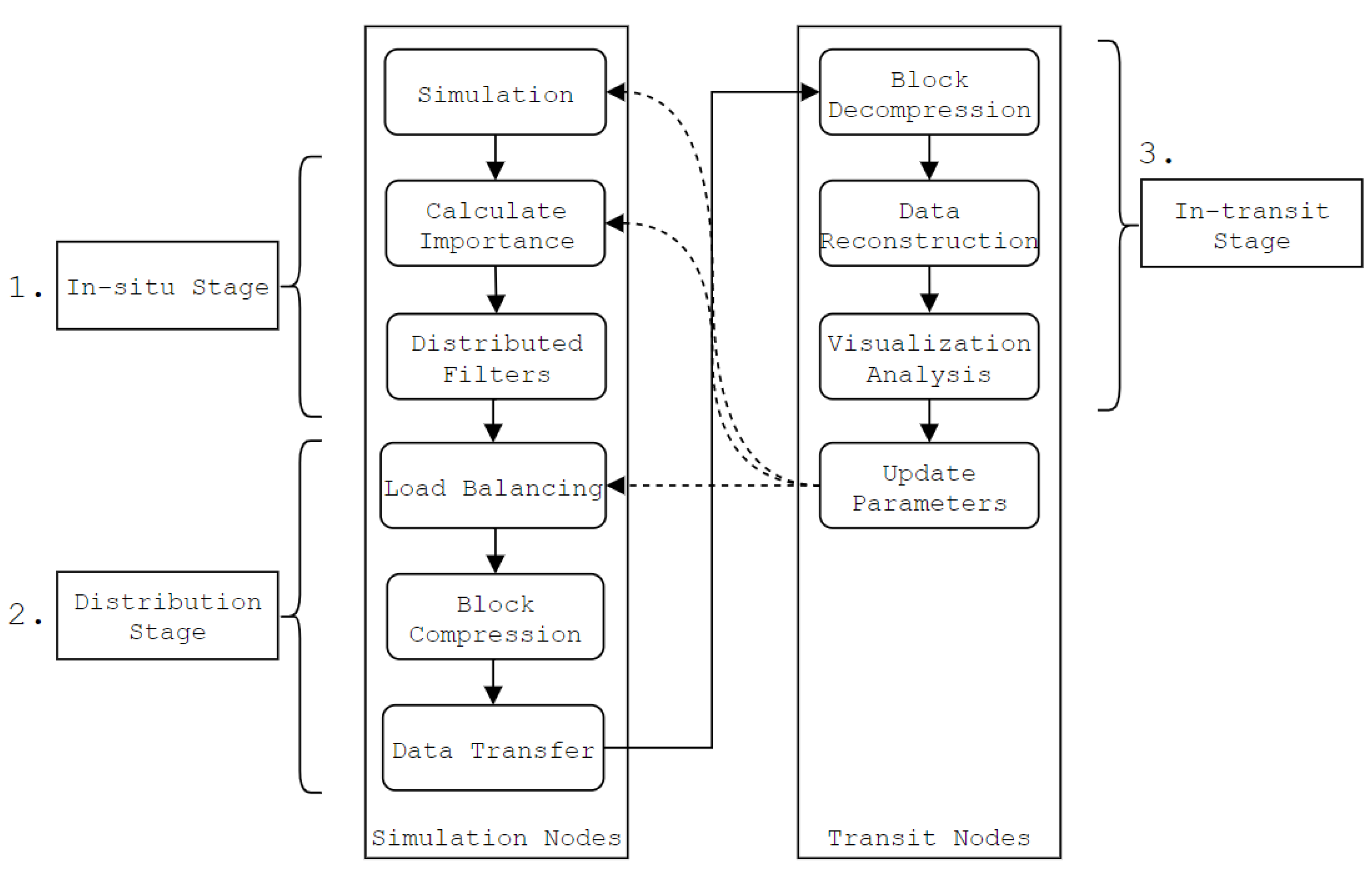
  • The in-situ stage (Section 3.1, Section 3.2, Section 3.3, Section 3.4), which consists of the proposed method. The block importance is calculated, and which compression method to use is determined on a per-block basis.
  • The distribution stage (Section 3.5), where data is compressed, load balanced and transferred over the network to the transit nodes.
  • The in-transit stage (Section 3.6), where compressed data is decompressed and restructured on the transit nodes.

3.1. Calculating Importance

Calculating block importance has been a time-consuming task in many related works, even for relatively small data sets. Because of this reason, the block importance in related work has generally been calculated using one or a few importance measurements. However, simulation data often contains many different types of regions of interest. Furthermore, the best compression algorithm might differ based on the entropy of the data in the different regions, meaning that there are many situations in which using multiple importance measurements would be preferable. Typically, the computation time would increase proportionally to the number of used importance measurements. However, in our solution, we strive to minimize this increase in computation time. In addition to performing importance calculations on a block’s complete simulation data, we also support using a random sample of a block’s data. That is to say, importance calculations can either be performed on the entire simulation data of a block or a smaller, random sampled subset of a block’s data. Using only a sample of the simulation data can result in a significant speedup. The calculated importance would not be entirely accurate, which might be an issue in specific applications. However, sampling could still be useful in most cases. For example, random sampling could be used to identify blocks that appear only to contain homogeneous space, i.e., blocks in which all values are identical. A non-sampled analysis of the data could then be performed on the subset identified by the sampled importance, which substantially could reduce the total computation time.
A key issue when calculating the importance is data locality. The simulated region is typically allocated in contiguous memory space. However, a block makes up a 3D subset of the simulated area, which leads to low cache hit rates, especially for small block sizes. Using multiple importance metrics or metrics that utilize advanced data access patterns further complicates this issue. Some related work [10] has solved this issue by assuming the simulated region is allocated on a per-block basis. However, we feel that this is too limiting. Our solution is to dynamically allocate and deallocate a separate buffer for a block or a block sample when it is analyzed. All relevant importance analyses are then applied in sequence on a per-block basis, which leads to higher cache hit rates and low memory overhead. Furthermore, this approach ensures that simulation data of each analyzed block only needs to be allocated and copied once, minimizing the computation time overhead introduced by this step. Operating on a separate buffer of a block’s subset of the simulated area leads to a much higher data locality, which means that multiple importance calculations can be performed at a lower computational cost.
A pipeline consists of a list of filters, which are executed in sequence. Filters contain probes, which are functions that analyze the data on a per-block basis. An overview of a pipeline’s block importance analysis scheme is provided in Algorithm 1.
Algorithm 1 Scheme used to calculate the importance of all blocks. The importance is used to determine the action of each block.
  • Require:
  •       B = { 1 , 2 , , N } : set of all N blocks
  •       F : set of all active filters in pipeline
  •       W = { w p } : set of weights, where w p is the weight of probe p
  • Ensure:
  •       I = { i 1 , i 2 , , i N } : set of importances, where i b is the importance for block b B
  •       A = { a 1 , a 2 , , a N } : set of actions, where a b is the action for block b B
  • 1: for each block b B  do
  • 2:      i b 0 ;                                                                                                                ▹ Importance initially set to zero for block b
  • 3:      a b NONE;                                                                                                         ▹ Action initially set to NONE for block b
  • 4:     for each filter f F  do
  • 5:         if  a b is in the scope of f then                                                                          ▹ Each scope is a set of zero or more actions
  • 6:            for each probe p of filter f do                                  ▹ p { Mean, Range, SD, AVGSEQ, Distinct, Entropy }
  • 7:                if p analyzes a sample which is not allocated then
  • 8:                    allocate sample of block b;
  • 9:                if p analyzes a block which is not allocated then
  • 10:                    allocate block b;
  • 11:                i b = i b + p ( b ) / w p ;                                            ▹ p ( b ) calculates the importance for probe p on block b
  • 12:            if  i b satisfies the condition of filter f then
  • 13:                 a b action of filter f;                                                                        ▹ a b { NONE, Skip, RLE, LZ77, HOMO }
  • 14:     Free the allocated memory of block b;
  • 15: return I , A ;
A filter contains zero or more probes, which are used to analyze each block in sequence. Each probe executed by a filter is assigned a custom weight (by default, 1). Given a block b, a filter f and a set of probes for filter f, P f , the resulting importance of block b, i b , after a filter has been applied is
i b = p P f p ( b ) w p ,
where w p is the weight of probe p and p ( b ) is the function by probe p to calculate the block importance of block b. A filter also contains an action, a condition, and a scope. An action specifies how a block should be handled during the data transfer stage. By default, a block has no specified action. However, a block’s action can be changed by a filter to, for example, use a specific reduction strategy during the data transfer stage. Whether a block should assume a filter’s action depends on if the block’s importance fulfills the filter’s condition. The condition returns either true or false depending on a block’s importance; for example, a condition could specify i b > 0.8 , in which case all blocks with importance higher than 0.8 will assume the filter’s action. The scope, a set of one or more actions, determines which blocks should be processed by a specific filter. For a filter to be applied, the block’s action needs to match one of the scope’s actions. This structure makes it possible to target specific subsets of blocks to perform further analysis and importance calculations.
Data is analyzed by using probes. Probes are short functions that analyze and output the importance of each individual block, based on the full content or a sample of a block. That is to say, the output of a probe calculating the mean value of a block is computed by iterating through each element in the block and then calculating the average value. In our testing, six different probes were used. The six probes are defined as follows:
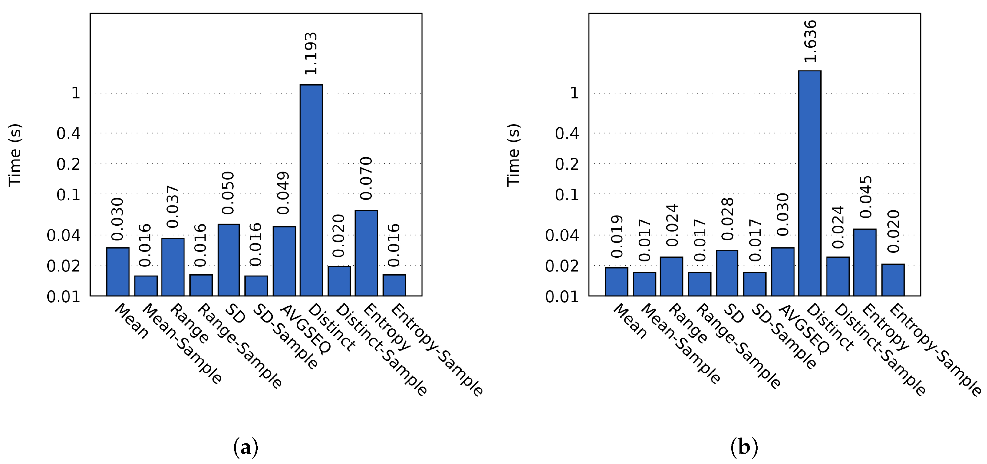
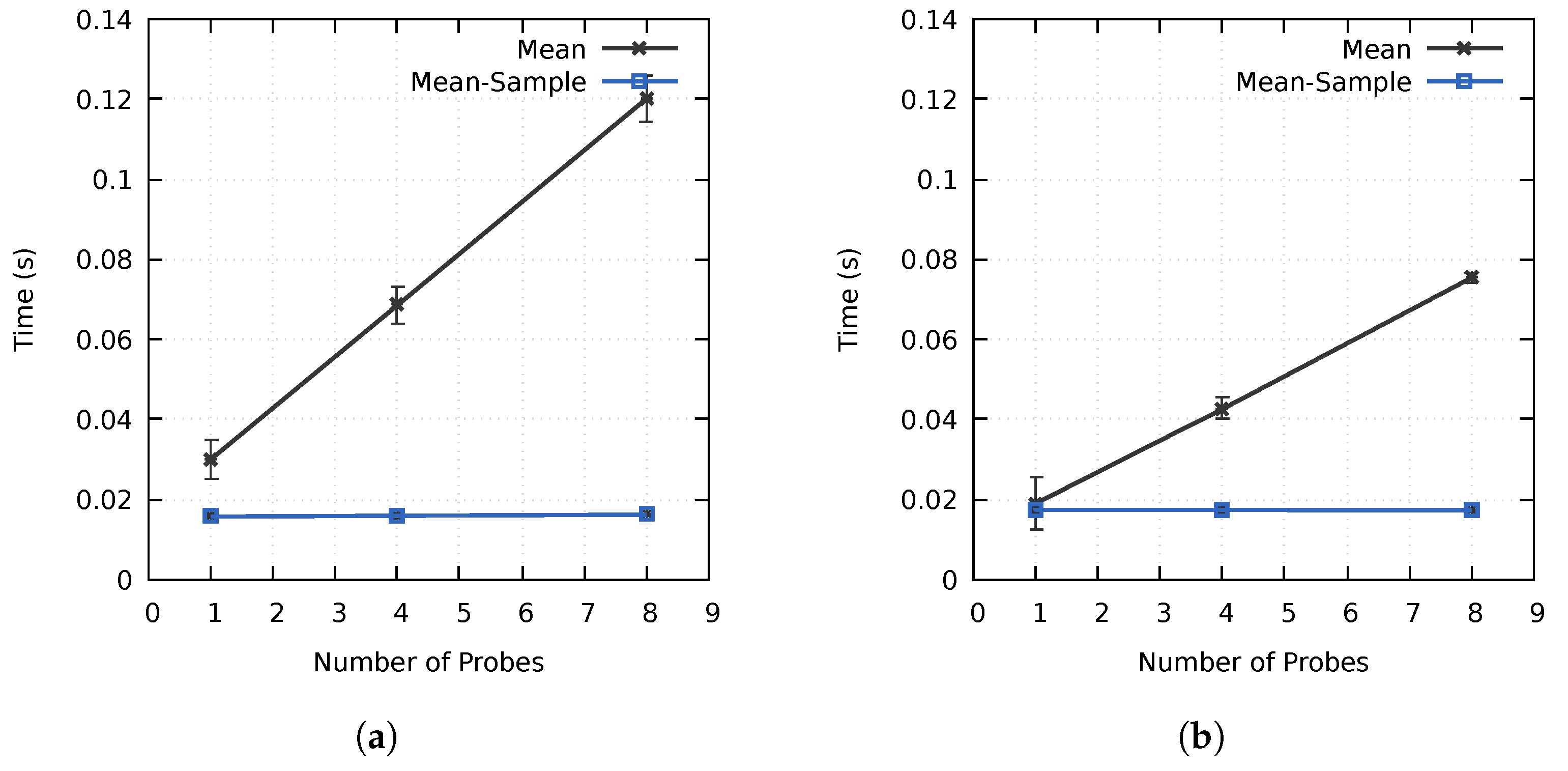
  • Mean. Calculates the mean of all values in a block.
  • Range. Calculates the range of the values in a block.
  • SD. Calculates the standard deviation of the values in a block.
  • AVGSEQ. Calculates the average sequence length of identical values in a block. This probe is only used on non-sampled data, as sampled data would not retain enough information about the average sequence length.
  • Distinct. Calculates the number of distinct values compared to the total number of values in a block.
  • Entropy. Calculates the entropy of a block [10].

3.2. Block Actions

Block actions consist of three stages: initialization, pre-processing, and post-processing. Block actions can act as tags for a wide variety of acceleration purposes, and can be seen as the action that has been taken for a specific block, based on its importance and the used filter conditions. However, in the context of this paper, we consider actions as tags for different types of compression methods. The initialization stage can be used to initialize resources and to specify the estimated compressed data size. Such information could be used to, for example, improve load balancing. The pre-processing and post-processing stages can be used to compress and decompress a block’s data, respectively. Five different actions are used in our testing:
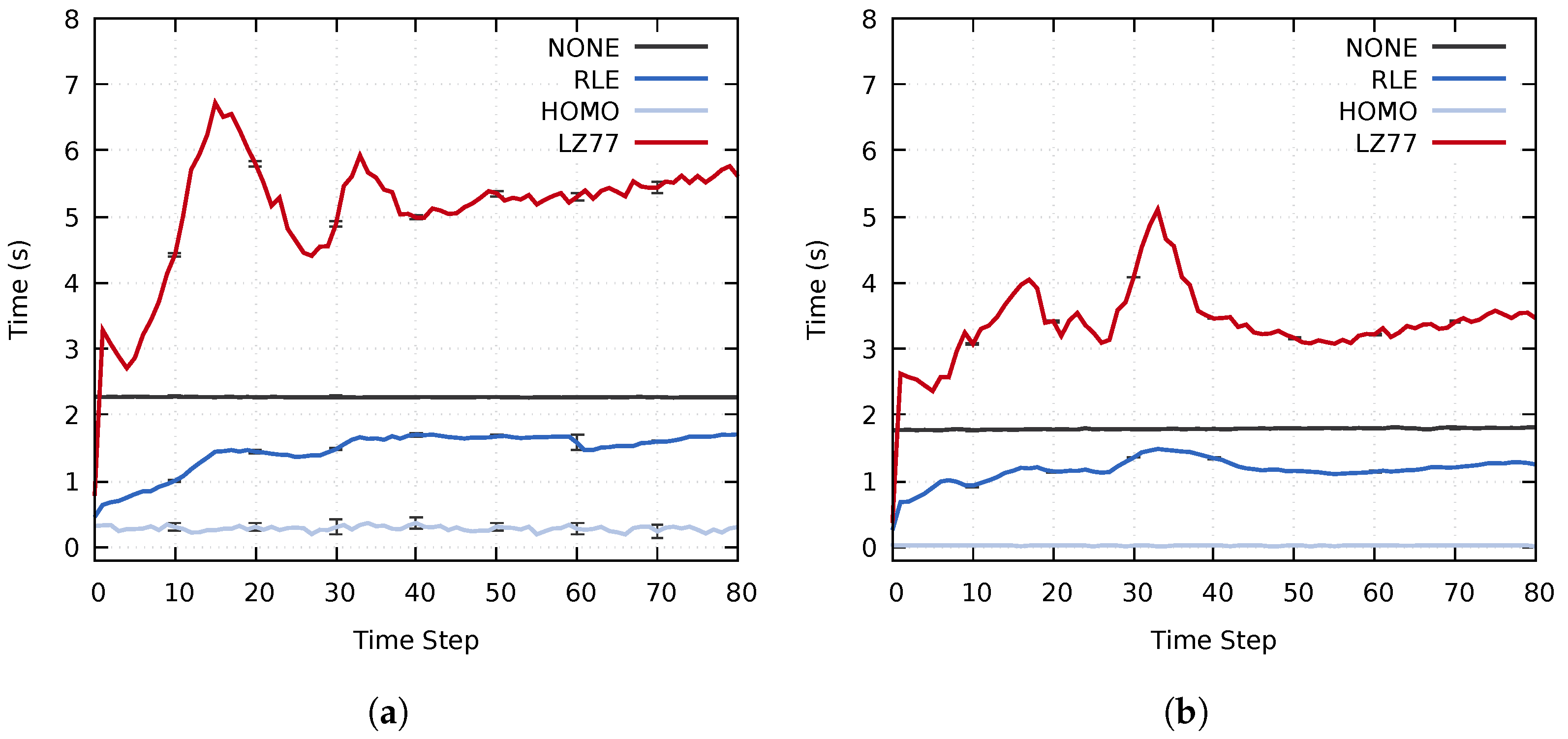
  • No Action (NONE). No reduction or compression is performed. Blocks have this action set by default. This action is mainly useful for blocks where the time overhead introduced by compression outweighs the speedup of data transfers.
  • Skip. Blocks with this action are never allocated or sent to the transit nodes. This action is useful if, for example, a region of the simulated grid is not of interest. Using the Skip action can, as such, substantially reduce the data transfer and co-processing times in some scenarios.
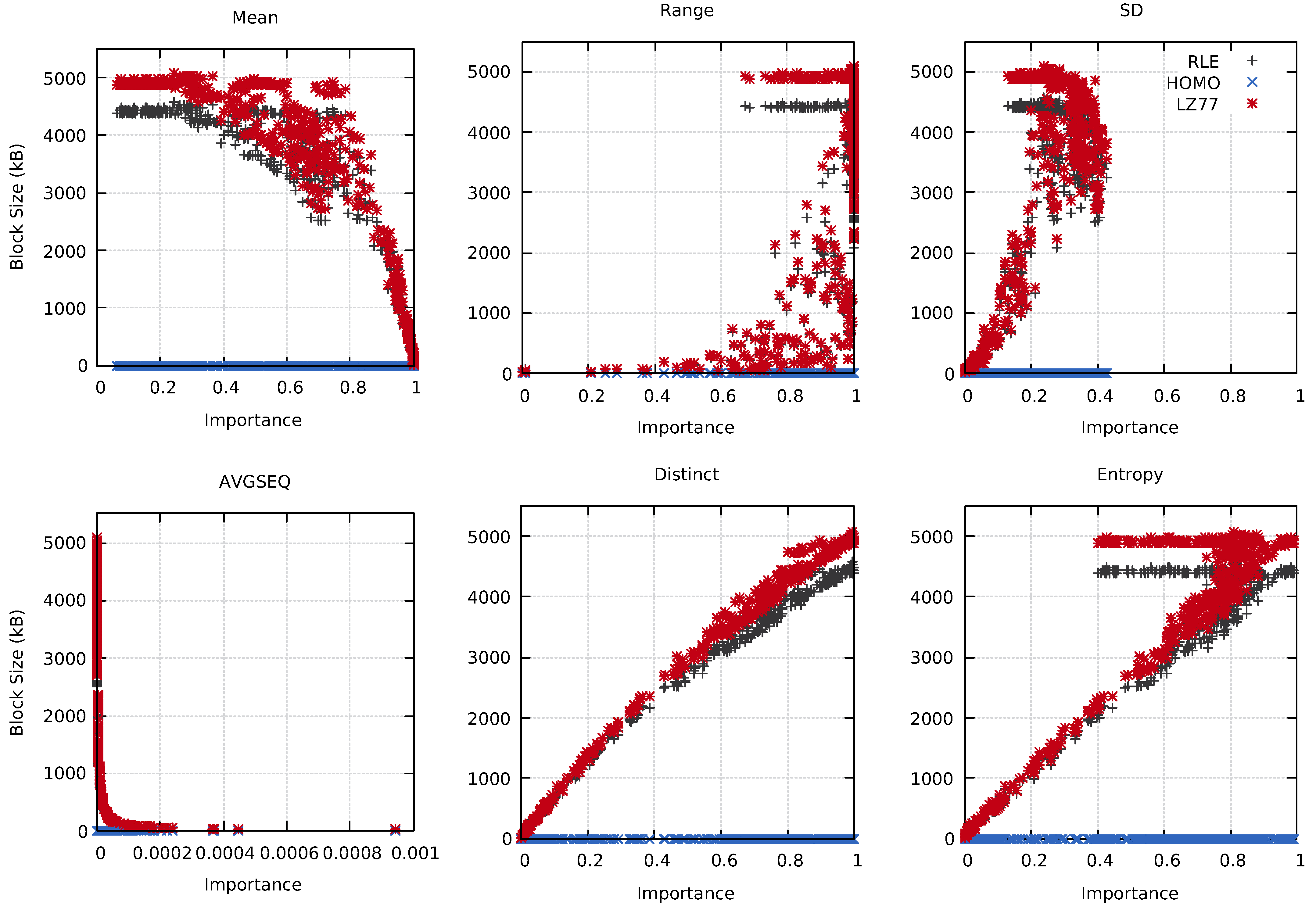
  • Run-Length Encoding (RLE). Blocks with the RLE action are compressed using RLE. Both the compression and decompression of data can be completed in one pass.
  • LZ77. Block with this action are compressed using the LZ77 compression algorithm [32]. Compared to the RLE compression method, LZ77 can be used to more effectively compress repeating sequences of data. This means that its usefulness differs depending on the simulation as well as on each individual block.
  • Homogeneous (HOMO). Blocks that are Homogeneous are allocated as a single value. Similarly to the Skip action, it can dramatically reduce the data transfer time. This action is useful for empty or homogeneous space, and can also be used to reduce regions that are not of interest. The main benefit that the Homogeneous action has over other types of compression and reduction algorithms is the compression time, which has a time complexity of O ( 1 ) .
We note that although these compression and reduction methods are used in the context of this paper, the proposed approach can be used in combination with any existing compression and reduction methods, including lossy methods like zfp [30], SZ [33], and its extension [31].

3.3. Adaptive Condition Window

The time required to perform importance calculations and data transfers largely depends on the filters and the target block actions, which are based on the specified filter conditions. Setting static filter conditions, i.e., each condition has a non-changing, constant value, could work in some situations. However, simulation data is rarely the same between any two time steps. As such, the execution time and memory usage could vary substantially. Instead, it could be preferable to adaptively change the parameters of the filter conditions based on some criterion. This criterion could be based on, for example, the execution time, memory usage, or the remaining allocated time on a compute cluster. We refer to this kind of filter condition as an adaptive condition.
In our approach, we have to consider multiple filters, all of which could include adaptive conditions. The key issue is how to adaptively modify the conditions without affecting the intended flow of the analysis. Our solution is to use an adaptive condition window, ω , by which multiple adaptive condition values can vary predictably. The condition window is a value that slides between 0.0 and 1.0, at 0.05 intervals. The condition window can slide one interval towards 0.0 or 1.0 after each time step. All filters have a defined range (upper bound u and lower bound l) for their condition value. The filter condition values are reevaluated after each executed time step based on input to the program, using the expression
l + ( u l ) · ω .
The upper and lower bounds can be set to the same value, in which case the condition value of that filter is constant.
For example, a researcher could determine that as much important data as possible should be saved to permanent storage after each time step. However, there is a strict time limit for the length of the I/O operation. The researcher would first decide on probes and filters that accurately can identify important data for the specific use case. The l and u variables would then be set to 0.0 , 1.0 , respectively. Initially, ω is set to 0.0 . However, after each time step, ω can increase by 0.05 based on if the I/O time exceeds the specified time limit. Over time, ω moves to the highest value possible such that the I/O operation does not exceed the time limit. As a result, the researcher can maximize the amount of data that can be stored for each time step. This behavior further scales to work with multiple probes and filters, meaning that many decisions can be made about different aspects of the simulation data.
The adaptive condition window ensures that the condition values of all filters can be modified in a controlled manner, thus retaining the intended analysis flow. One condition window is used per pipeline, meaning that different condition windows can be used for different data sets if required.

3.4. Advantages of the Pipeline Structure

The proposed structure facilitates pipeline construction in practical applications. Specifically, the pipeline has three key advantages compared to alternative structures (e.g., a directed acyclic graph (DAG) or a decision tree approach [34] that calculates an importance metric on each branch node):
  • Ease of use. Using the structure of the proposed pipeline, each component (e.g., a filter or probe) is categorized and serves a clear purpose. In practice, it is easy to construct and understand the structure of the proposed pipeline. In contrast, some structures (e.g., decision trees) would not be intuitive without a visual interface.
  • Gradual refinement. A new action can be assigned to a block after each filter has been applied. As filters are applied in sequence, this behavior enables a gradual refinement of the importance analysis. More advanced or time-consuming analyses can be limited to the relevant subsets of the simulation data. Although this behavior can be mirrored by other structures (e.g., a DAG or tree structure), it would be more complicated to create.
  • Reusability. It is easy to reuse parts of a pipeline (e.g., filters or probes) in other applications as all parts of the pipeline are compartmentalized.

3.5. Data Distribution

Load balancing blocks of 3D data sets has been the focus of extensive research [10,35,36,37,38,39,40]. A load balancing technique can either create a static distribution of the data or dynamically change the distribution based on some variables. Typically, dynamic load balancing techniques strive to minimize either the difference in computation time or the difference in memory usage on each process.
Scientific simulations often generate large quantities of data, meaning that memory usage is of primary concern. Therefore, we currently consider a static and a dynamic different load balancing technique. The static technique is based on the initial distribution in a k-d tree [41], which distributes blocks to all processes on the transit nodes. However, some blocks may have been removed using the Skip action. As such, using this technique could result in a memory imbalance on the transit nodes. The dynamic technique partly resolves this issue by rebalancing the k-d tree. Let B t be the list of blocks on transit process t, μ the average number of blocks per process, and n the number of transit processes. The goal is then to minimize
t = 1 n | B t | μ n ,
i.e., the difference in allocated memory on each process on the transit nodes.
Blocks sent to a specific process on a transit node make up a contiguous and convex subset of the original 3D data set. They can, as such, be decompressed in parallel and combined to reconstruct a single region in 3D space. This step is essential to perform certain types of analyses and visualizations efficiently. For example, many volume rendering engines utilize internal block structures to perform empty space skipping [42] and optimization techniques such as early ray termination [43,44]. Prematurely partitioning the 3D data set into multiple blocks can negatively affect the effectiveness of such techniques.
At the start of the distribution stage, we utilize distributed filters to apply filters that require information about blocks from multiple processes. For evaluation, only one distributed filter is used, Filter Borders. The Filter Borders distributed filter attempts to identify blocks of a specific action on the border of the 3D data set. If a slice of border blocks can be identified, their action is changed to the target action specified by the filter. For example, this distributed filter can be used to identify slices of homogeneous blocks along the border of the 3D volume, and then exclude them from the in-transit rendering process by changing the action to Skip.

3.6. In-Transit Co-Processing

Blocks transferred to processes on transit nodes might have been reduced or compressed during the in-situ stage. To perform any visualization or analysis of the data, the blocks first need to be decompressed. Blocks are decompressed based on the used compression algorithms. Because blocks on a specific process make up contiguous and convex regions in 3D space they can also easily be aggregated into a single block, which significantly can improve the performance of the co-processing process.
The content of the co-processing is not part of our proposed approach. Instead, the approach only handles data decompression and data reconstruction on the transit nodes. Analysis and visualization can be performed in a normal fashion according to the researcher’s needs, without any need to integrate existing tools and software with our approach.

4. Experimental Evaluation

To evaluate the proposed method and the approach to accelerate in-transit co-processing, we have run a series of tests on two different compute clusters, cluster A and cluster B (Octopus) [45], at different resolutions using up to 864 cores. Information about the test environments is detailed in Table 2.

4.1. Experiment Description
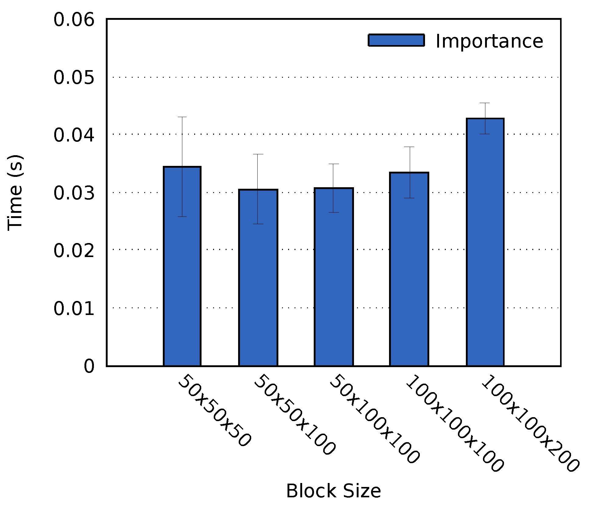
We used the RMI simulation data to evaluate the performance of our proposed approach. The RMI test-case set-up as well as numerical methods considered are similar to previous work [46,47]. However, here, the effect of the membrane mesh separating the two gases is modelled in the simulations according to well-defined modes combined with random perturbation components [48,49].
To mimic a realistic co-processing scenario, we used up to three different variables in each analyzed time step: the mass fraction (MF) and two axes of the momentum (MY and MZ). The data of these variables were analyzed, compressed, and transferred to the transit nodes using the proposed approach. On the transit nodes, data decompression and data reconstruction were also performed. However, no additional co-processing was included as part of the testing.
A grid resolution of 1601 × 401 × 801 was used on cluster A, resulting in 11.5 GB of data spread over three variables, each time step. Similarly, the grid resolution on cluster B was set to 2401 × 601 × 1201 , resulting in 38.7 GB of data for the three analyzed variables.
We chose to perform co-processing for time steps at a 5 × 10 5 second interval (simulated time). In practice, this amounts to approximately 1 out of every 127 and 1 out of 193 time steps, respectively. The simulations ran for 10,292 time steps on cluster A and 15,653 time steps on cluster B, out of which 81 were analyzed. That is to say, up to 0.91 TB (cluster A) and 3.06 TB (cluster B) of data were analyzed. It took a total of 117.5 h on cluster A and 100.9 h on cluster B to run the simulations.
The data was loaded into memory as 64-bit floats during the testing. Figure 3 shows a visualization of the MF data set, using the OSPRay rendering engine [20], version 1.7.3.
The proposed approach can utilize a combination of existing compression methods, and its performance depends on the performance of the used methods. We, therefore, chose to compare the approach to uniformly applying each compression method used by the approach on the full data set. In the context of this paper, those methods consist of RLE, LZ77, and HOMO, as specified in Section 3.2.

4.2. Block Size

Analysis operations are heavily dependent on the size of each individual block. Appropriate block sizes for volume rendering has been investigated in related work [36], which found that blocks with a 64 × 64 × 64 resolution achieved the best result in their use case. A similar block resolution has been used in research related to this work [10], although with no motivation. We analyzed five resolution to determine an appropriate block resolution for our use case: 50 × 50 × 50 , 50 × 50 × 100 , 50 × 100 × 100 , 100 × 100 × 100 , and 100 × 100 × 200 .
Tests were performed on cluster A using the MF data set and a Mean probe. As per the results, shown in Figure 4, a block size of 50 × 50 × 100 or 50 × 100 × 100 achieved the fastest computation time. We chose to use the block size of 50 × 100 × 100 in all successive tests on cluster A presented in this paper. The simulation resolution and the number of processes on cluster B differ from that of cluster A. As a result, it was not possible to use the same block size. Instead, we set the block size on cluster B to 75 × 75 × 75 , which was the closest alternative.

4.3. Performance of the Proposed Method

The computation time varied between different probes, as shown in Figure 5. For sampled probes we used a block sample size of 2390 and 2387 for the two respective resolutions. All sampled probes were consistently faster; the best example being the Distinct probe, which on average took 1.19 s to complete on cluster A. In comparison, the sampled Distinct probe only required 0.02 s of computation time (a speedup of 61.14). Similar results were obtained on cluster B.
We observe that the sampled probes generally were able to achieve more significant speedups on cluster A. This is primarily because of two reasons. First, simulation processes on cluster A had to process more data than the processes on cluster B. Second, simulation processes on cluster B could more efficiently calculate the importance due to having access to more cores. Calculating the importance of sampled blocks is limited by the time required to complete the initial data access, which is similar on both clusters.
As discussed in Section 3.1, one of the goals of the proposed method was to minimize the computation overhead of utilizing multiple probes. As seen in Figure 6, the computation time increased linearly when using multiple non-sampled Mean probes. However, increasing the number of probes from one to four and eight only increased the computation time on cluster A by 2.28 × and 4 × , respectively, and 2.24 × and 3.96 × on cluster B, as compared to the expected 4 × and 8 × . Similarly, the increase was only 1% and 3% for the sampled Mean probes on cluster A, whereas all results were within the margin of error on cluster B. By preprocessing the block data and using the block-based importance calculation process described in Section 3.1, the importance calculation time is not directly proportional to the number of used probes. This is especially the case for sampled probes, where the increase in computation time was negligible in our tests. The initial data reorganization required to achieve this performance results in some overhead, increasing the computation time for a probe with a simplistic data access pattern. However, as seen in Figure 6, the performance is better when using multiple probes or probes with more advanced data access patterns as a result of the improved cache hit rate. The performance of our method is directly affected by the data access pattern of the used probe(s). Intuitively, probes with advanced data access patterns should benefit more from the higher cache hit rates and improved data locality. A one-pass algorithm, such as the Mean probe, should as such represent a worst-case scenario.
The accuracy of the sampled probes depends on the sample size as well as the used probe algorithm. Table 3 shows the absolute error, E, of the sampled probes using the MF data set on cluster A at time step 80. E is equivalent to x i x , where x i and x are the measured and true values, respectively. Using the Mean or SD sampled probes resulted in all blocks having an importance value within 0.01 of the correct importance value. However, The Range and Distinct sampled probes were not as accurate as the Mean, SD, and Entropy probes. In some scenarios, the calculated importance of these probes depends on a small subset of the data. For example, by changing a single data value in some blocks, the importance calculated by the Range probe can increase from 0 to 1.
In summary, the importance analysis scheme could successfully improve the performance when using multiple probes. Sampled probes could achieve a high accuracy and further accelerate the importance analysis computation.

4.4. Evaluating the Proposed Approach

In this section we evaluate the performance of the approach used to accelerate in-transit co-processing. The compression performance is discussed in Section 4.4.1, whereas its ability to accelerate the execution time of the co-processing of the RMI simulation is discussed in Section 4.4.2.

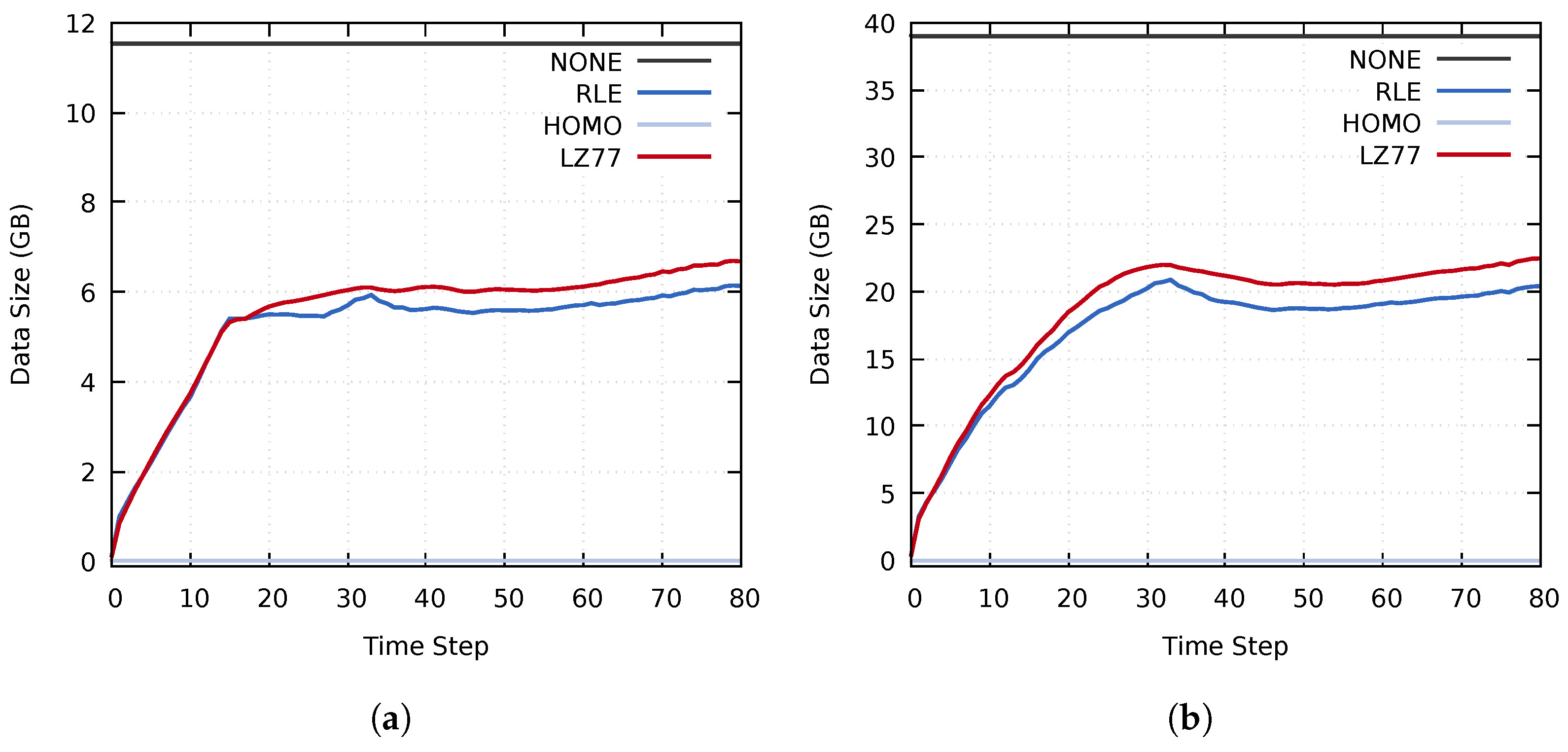
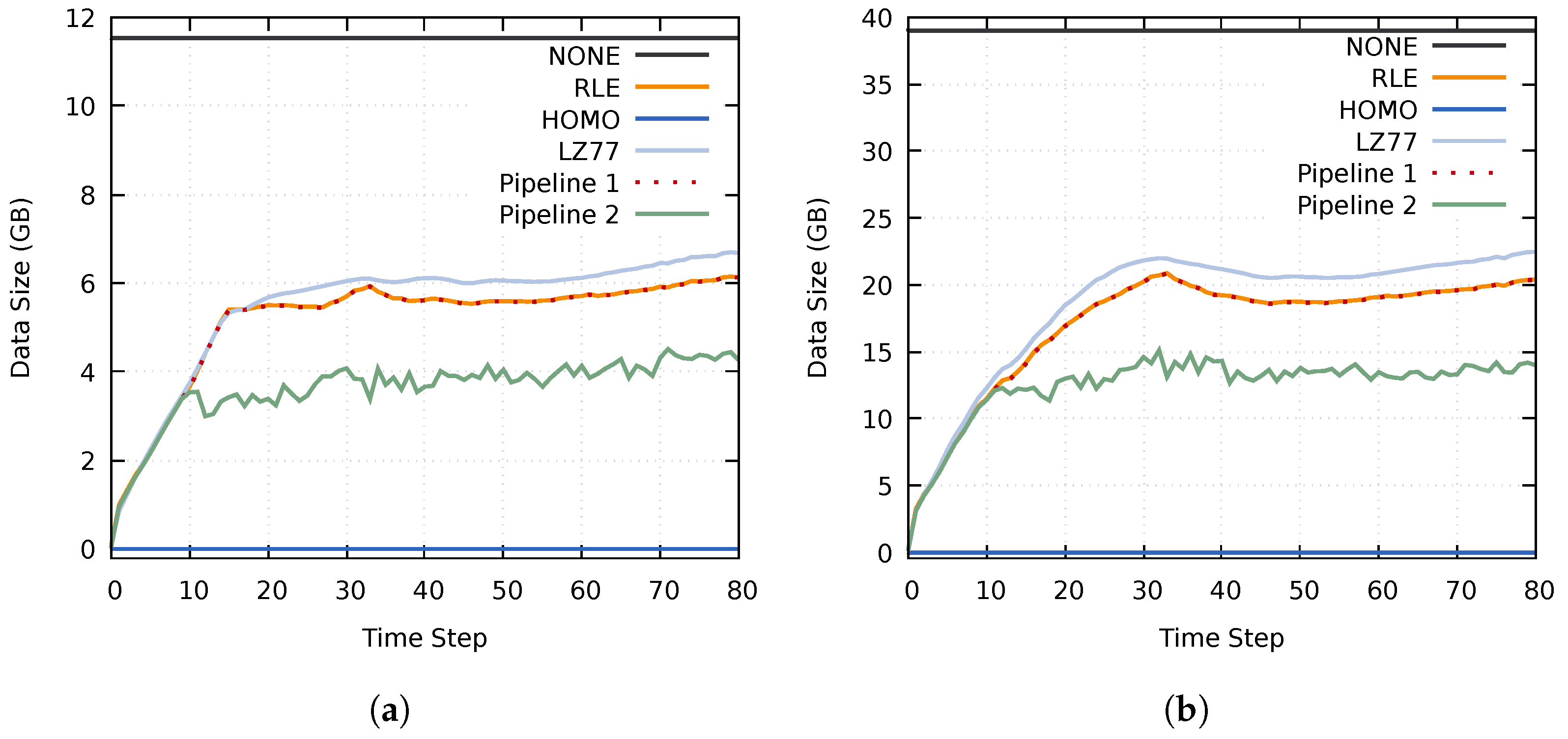
4.4.1. Compression Performance

Intuitively, different probes should reflect different information about the underlying block data. It should then be possible to use this information to, for example, select the best compression technique for a specific use case. Figure 7 shows the relation between the RLE-, HOMO-, and LZ77-compressed block sizes and the importance calculated by the used probes. The Distinct probe provided an almost linear relationship between the importance and the compressed data size, as seen in the figure. Similarly, the AVGSEQ and Entropy probes had clear connections between their calculated importance and the compressed block sizes.
The compressed data size achieved by using RLE compression was generally smaller than when using LZ77. This trend was caused by the entropy of the used data set, which does not contain many repeating sequences of values. Similarly, the effectiveness of the RLE compression is linked to the many homogeneous regions in the investigated data set. However, as seen in Figure 8 and Figure 9, the performance of the various compression methods vary throughout the simulation. The initial data set, at time step 0, contains many homogeneous regions. Consequently, the initial compressed data size is minimal. As the simulation progresses, the homogeneous regions become smaller and disappear, which increases the compressed data size. The total compressed data size remains lower than that of the uncompressed data throughout the simulation. However, for some blocks, the compression time overhead becomes higher than the speedup of data transfers, as seen for the RLE method in Figure 8. This further reinforces our notion of selectively choosing which compression method to use on a per-block basis for each time step.

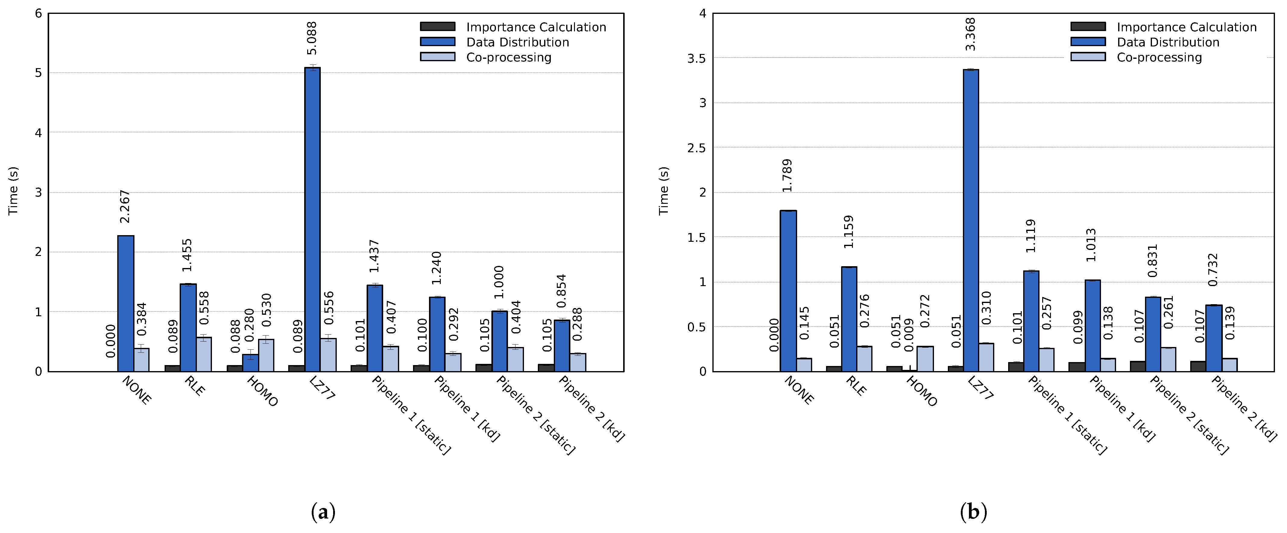
4.4.2. Assessing the Execution Times of the Proposed Approach

Pipelines should be devised based on the needs of the researcher and the nature of the used simulation. It is not possible to create a pipeline that is optimal in all scenarios. Furthermore, which compression methods to use also depend on the specific use case. We designed two advanced pipelines: one lossless and one lossy which uses a condition window to reduce the least important data adaptively. Both pipelines used a distributed filter to remove homogeneous border blocks (i.e., block which are not of any significance to the analysis of the simulation data). Furthermore, the pipelines were evaluated using both no load balancing (static) and a k-d tree load balancing technique (kd) to equalize the data distribution after the use of the distributed filter.
Pipeline 1 is structured as follows. Initially, all blocks are sampled using the Range probe. Blocks with an importance of 0 have their actions set to RLE. A non-sampled Range probe is then used on all blocks with action RLE. If the importance is 0, the action is set to Homogeneous. By initially using a sampled probe, the non-sampled probe only has to operate on a subset of all blocks, which reduces the computation time. Finally, the third filter uses a sampled Distinct probe to change the action of blocks with the NONE action and an importance ≤0.9 to RLE. The value 0.9 is based on previous experiments to evaluate the compressed block sizes, displayed in Figure 7. Using the Distinct probe, having importance lower than approximately 0.9 resulted in a lower block size than the original non-compressed data. Intuitively, blocks with many distinct values might also be more time-consuming to compress and decompress, further increasing the data transfer time. We chose to use a sampled version of the Distinct probe to accelerate the in-situ computation time. Note that the resulting compression of Pipeline 1 is lossless.
The idea behind Pipeline 2 is to reduce the most unimportant data (in this case, the blocks containing the lowest amount of distinct values) on-the-fly to achieve a total compressed data size of between 1200 to 1600 MB (cluster A) and 4000 to 5400 MB (cluster B) for each data set (i.e., using all three data sets, up to 4.69 GB and 15.82 GB of data for each time step on clusters A and B, respectively). We use a range rather than a specific threshold to reduce the volatility of the compressed data size between each time step. The initial three filters of Pipeline 2 are identical to those of Pipeline 1. However, Pipeline 2 includes a fourth filter that utilizes a condition window. The filter uses a Distinct sampled probe, and targets blocks with the RLE or NONE actions. The condition value range is set as [0, 1.0], with an initial value of 0. If the condition of the filter is fulfilled, the action is changed to Homogeneous.
The data size of homogeneous blocks using the Homogeneous compression method was almost the same as when using RLE compression. This can be seen in Figure 10, where the compressed data size of Pipeline 1 is almost identical to when utilizing an RLE compression. However, Pipeline 2 achieved a significantly lower data size because of the additional adaptive (lossy) reduction filter. Noteworthy is that Pipeline 2 never reached the upper limits of 4.69 GB and 15.82 GB. This is because the compressed data size of at least one data set remained below the specified upper data size threshold.
The impact of the proposed approach on the entire simulation time widely depends on the used simulation and co-processing. For example, the simulation time of a single time step, detailed in Section 4.1, and the in-transit co-processing time can vary by orders of magnitude depending on the simulation, the specified simulation parameters and which types of analysis and visualization tasks are performed during the co-processing stage. Furthermore, co-processing could be performed for each simulated time step or for a small fraction of time steps. As such, we chose to focus the evaluation exclusively on the actual performance of the three main stages of the proposed approach, i.e., the co-processing stage only consists of data decompression and data reconstruction. The average execution times of each stage are shown in Figure 11. The importance calculation of the RLE, HOMO, and LZ77 tests used for comparison consisted of a single Mean probe.
Out of the lossless compression methods used for comparison, RLE achieved the best performance. For the total execution time, the RLE compression method achieved a speedup of 1.26 × (cluster A) and 1.3 × (cluster B) compared to using no compression. The lossless Pipeline 1 achieved an even more significant speedup; 1.62 × on cluster A and 1.55 × on cluster B. Compared to RLE, Pipeline 1 could speed up the execution time by up to 1.29 × and 1.19 × on the two respective clusters. Similarly, Pipeline 2, which reduces unimportant data, achieved total speedups of 1.69 × and 1.52 × compared to the RLE method. Table 4 summarizes the average speedups of the total execution time for both pipelines compared to the other evaluated methods.
In more detail, both Pipeline 1 and Pipeline 2 achieved significantly better performance for the data distribution and co-processing stages than the NONE, RLE, and LZ77 methods. The execution time of the co-processing stage for Pipeline 1 was similar to the RLE test when using static load balancing. The uneven load caused this; although multiple transit processes achieved significantly lower computation time than when using only RLE compression, the total execution time is dependent on the slowest process. Using a k-d load balancing technique solved the uneven load on the transit nodes. On cluster A, Pipelines 1 and 2 achieved speedups of 1.91 × and 1.94 × of the co-processing stage as compared to using RLE compression, and speedups of 1.32 × and 1.33 × compared to using no compression. Similarly, on cluster B the two pipelines achieved speedups of 2.00 × and 1.99 × as compared to an RLE compression. Compared to using no compression, the speedup of the co-processing stage was 1.05 × and 1.04 × for the two respective pipelines.
Utilizing dynamic load balancing significantly improved the execution times of the co-processing stage. However, the load balancing only determines where data is sent. The compression time and the amount of data that needs to be transferred from each simulation process do not change. Using a dynamic load balancing technique did not improve the execution time of the data distribution stage to the same extent. On cluster A, the two pipelines achieved speedups of 1.17 × and 1.70 × as compared to an RLE compression and speedups of 1.83 × and 2.65 × compared to using no compression. On cluster B, the pipelines achieved speedups of 1.14 × and 1.58 × compared to RLE compression and speedups of 1.77 × and 2.44 × compared to no compression.
Interestingly, the lossless Pipeline 1 was able to achieve better performance in all aspects (the compressed data size and the compression, data transfer, and decompression times) than the other lossless compression methods. This results from the fact that both of the pipelines scale with the utilized compression methods; in this case, using NONE, RLE, and HOMO. This scaling can be seen in Figure 10, where the compressed data size of Pipeline 1 closely follows that of the RLE compression. This behavior should extend to other compression methods as well.

5. Conclusions

In this paper, we have presented a method to efficiently determine the importance of regions of interest of simulation data, emphasizing on using multiple importance metrics. In addition, we have presented a use case where the method was used to accelerate the in-transit co-processing of an RMI simulation by lowering the data transfer time. The approach to accelerate in-transit co-processing uses the importance of regions of interest to determine how to best combine the usage of multiple different compression methods on different subsets of the simulation data. Simulation data is analyzed to determine the importance of all regions of the 3D data sets, which is then used as a basis to utilize multiple compression and reduction methods adaptively.
We have evaluated the performance of the proposed method and approach by conducting tests on two different compute clusters, using multivariate data from an RMI simulation. Our proposed method was able to expeditiously calculate block importance, even when multiple data probes were used. The above was especially the case for probes using sampled data, which could calculate accurate importance values at a much faster rate. The proposed method was also able to adaptively identify regions of important data in a reliable manner. The excellent scalability when using multiple data probes and low computation times also make the method viable to be used in many other in-situ and in-transit scenarios, such as: guiding the simulation; saving important data to permanent storage; or in tandem with additional analysis or visualization software. As for the approach, we were able to achieve better performance in all aspects (the compressed data size and the compression, data transfer, and decompression times) than the compression methods used for comparison. Compared to an RLE compression, using the proposed approach in a lossless scenario resulted in a speedup of up to 1.29 × for the overall execution time, and 2 × when performing data decompression. We conclude that the proposed approach significantly can accelerate the in-transit co-processing process.
In future work, we will investigate how the proposed method can be used for other use cases. Furthermore, we plan to extend the proposed approach to work better with in-situ co-processing workflows.

Author Contributions

Conceptualization, M.W.; methodology, M.W., D.D. and I.K.; software, M.W., D.D. and I.K.; validation, M.W., D.D. and I.K.; formal analysis, M.W.; investigation, M.W.; resources, M.W., F.I., M.O. and D.D.; data curation, M.W., F.I. and M.O.; writing—original draft preparation, M.W., D.D. and I.K.; writing—review and editing, M.W., F.I., D.D. and M.O.; visualization, M.W.; supervision, F.I. and D.D.; project administration, M.W.; funding acquisition, F.I. All authors have read and agreed to the published version of the manuscript.

Funding

This study was supported in part by the Japan Society for the Promotion of Science KAKENHI Grant Numbers 20K21794.

Institutional Review Board Statement

Not applicable.

Informed Consent Statement

Not applicable.

Data Availability Statement

Not applicable.

Acknowledgments

The work was partly achieved through the use of the Octopus cluster at the Cybermedia Center, Osaka University. We would like to thank JHPCN and the Cybermedia Center at Osaka University for the generous use of the Octopus cluster.

Conflicts of Interest

The authors declare no conflict of interest.

References

  1. Moreland, K. The Tensions of In Situ Visualization. IEEE Comput. Graph. Appl. 2016, 36, 5–9. [Google Scholar] [CrossRef]
  2. Ma, K. In Situ Visualization at Extreme Scale: Challenges and Opportunities. IEEE Comput. Graph. Appl. 2009, 29, 14–19. [Google Scholar]
  3. Rivi, M.; Calori, L.; Muscianisi, G.; Slavnić, V. In-situ Visualization: State-of-the-Art and Some Use Cases. 2012. Available online: https://www.hpc.cineca.it/sites/default/files/In-situ_Visualization_State-of-the-art_and_Some_Use_Cases.pdf (accessed on 10 April 2021).
  4. Yu, H.; Wang, C.; Grout, R.W.; Chen, J.H.; Ma, K. In Situ Visualization for Large-Scale Combustion Simulations. IEEE Comput. Graph. Appl. 2010, 30, 45–57. [Google Scholar]
  5. Bennett, J.C.; Abbasi, H.; Bremer, P.; Grout, R.; Gyulassy, A.; Jin, T.; Klasky, S.; Kolla, H.; Parashar, M.; Pascucci, V.; et al. Combining in-situ and in-transit processing to enable extreme-scale scientific analysis. In Proceedings of the International Conference on High Performance Computing, Networking, Storage and Analysis (SC’12), Salt Lake City, UT, USA, 24–29 June 2012; pp. 1–9. [Google Scholar]
  6. Friesen, B.; Almgren, A.; Lukic, Z.; Weber, G.; Morozov, D.; Beckner, V.; Day, M. In situ and in-transit analysis of cosmological simulations. Comput. Astrophys. Cosmol. 2016, 3, 1–18. [Google Scholar] [CrossRef] [Green Version]
  7. Flatken, M.; Wagner, C.; Gerndt, A. Distributed Post-processing and Rendering for Large-Scale Scientific Simulations. In Scientific Visualization: Uncertainty, Multifield, Biomedical, and Scalable Visualization; Springer: London, UK, 2014; pp. 381–398. [Google Scholar]
  8. Moreland, K.; Oldfield, R.; Marion, P.; Jourdain, S.; Podhorszki, N.; Vishwanath, V.; Fabian, N.; Docan, C.; Parashar, M.; Hereld, M.; et al. Examples of in Transit Visualization. In Proceedings of the 2nd International Workshop on Petascal Data Analytics: Challenges and Opportunities (PDAC’11), Seattle, WA, USA, 14 November 2011; Association for Computing Machinery: New York, NY, USA, 2011; pp. 1–6. [Google Scholar]
  9. Kress, J. In-Line vs. In-Transit In Situ: Which Technique to Use at Scale? Ph.D. Thesis, University of Oregon, Eugene, OR, USA, 2020. [Google Scholar]
  10. Dorier, M.; Sisneros, R.; Gomez, L.B.; Peterka, T.; Orf, L.; Rahmani, L.; Antoniu, G.; Bougé, L. Adaptive Performance-Constrained In Situ Visualization of Atmospheric Simulations. In Proceedings of the 2016 IEEE International Conference on Cluster Computing (CLUSTER), Taipei, Taiwan, 12–16 September 2016; pp. 269–278. [Google Scholar]
  11. Wang, C.; Yu, H.; Ma, K. Importance-Driven Time-Varying Data Visualization. IEEE Trans. Vis. Comput. Graph. 2008, 14, 1547–1554. [Google Scholar] [CrossRef] [PubMed] [Green Version]
  12. Nouanesengsy, B.; Woodring, J.; Patchett, J.; Myers, K.; Ahrens, J. ADR Visualization: A Generalized Framework for Ranking Large-Scale Scientific Data Using Analysis-Driven Refinement. In Proceedings of the 2014 IEEE 4th Symposium on Large Data Analysis and Visualization (LDAV), Paris, France, 9–10 November 2014; pp. 43–50. [Google Scholar]
  13. Berger, M.J.; Oliger, J. Adaptive mesh refinement for hyperbolic partial differential equations. J. Comput. Phys. 1984, 53, 484–512. [Google Scholar] [CrossRef]
  14. Schive, H.; ZuHone, J.A.; Goldbaum, N.J.; Turk, M.J.; Gaspari, M.; Cheng, C. gamer-2: A GPU-accelerated adaptive mesh refinement code—Accuracy, performance, and scalability. Mon. Not. R. Astron. Soc. 2018, 481, 4815–4840. [Google Scholar] [CrossRef] [Green Version]
  15. Shimokawabe, T.; Onodera, N. A High-Productivity Framework for Adaptive Mesh Refinement on Multiple GPUs. In Proceedings of the International Conference on Computational Science (ICCS 2019), Faro, Portugal, 12–14 June 2019; pp. 281–294. [Google Scholar]
  16. Biswas, A.; Dutta, S.; Pulido, J.; Ahrens, J. In Situ Data-Driven Adaptive Sampling for Large-Scale Simulation Data Summarization. In Proceedings of the Workshop on In Situ Infrastructures for Enabling Extreme-Scale Analysis and Visualization (ISAV’18), Dallas, TX, USA, 12 November 2018; pp. 13–18. [Google Scholar]
  17. Dutta, S.; Biswas, A.; Ahrens, J. Multivariate Pointwise Information-Driven Data Sampling and Visualization. Entropy 2019, 21, 699. [Google Scholar] [CrossRef] [PubMed] [Green Version]
  18. Fabian, N.; Moreland, K.; Thompson, D.; Bauer, A.C.; Marion, P.; Gevecik, B.; Rasquin, M.; Jansen, K.E. The ParaView Coprocessing Library: A scalable, general purpose in situ visualization library. In Proceedings of the 2011 IEEE Symposium on Large Data Analysis and Visualization, Providence, RI, USA, 23–24 October 2011; pp. 89–96. [Google Scholar]
  19. Childs, H.; Brugger, E.; Whitlock, B.; Meredith, J.; Ahern, S.; Bonnell, K.; Miller, M.; Weber, G.H.; Harrison, C.; Fogal, T.; et al. VisIt: An End-User Tool for Visualizing and Analyzing Very Large Data. In Proceedings of the SciDAC, Denver, CO, USA, 10–14 July 2011. [Google Scholar]
  20. Wald, I.; Johnson, G.; Amstutz, J.; Brownlee, C.; Knoll, A.; Günther, J.J.J.; Navratil, P. OSPRay—A CPU Ray Tracing Framework for Scientific Visualization. IEEE Trans. Vis. Comput. Graph. 2017, 23, 931–940. [Google Scholar] [CrossRef]
  21. Meagher, D. Geometric modeling using octree encoding. Comput. Graph. Image Process. 1982, 19, 129–147. [Google Scholar] [CrossRef]
  22. Kageyama, A.; Yamada, T. An approach to exascale visualization: Interactive viewing of in-situ visualization. Comput. Phys. Commun. 2014, 185, 79–85. [Google Scholar] [CrossRef] [Green Version]
  23. Ahrens, J.; Jourdain, S.; O’Leary, P.; Patchett, J.; Rogers, D.H.; Petersen, M. An Image-based Approach to Extreme Scale in Situ Visualization and Analysis. In Proceedings of the International Conference for High Performance Computing, Networking, Storage and Analysis (SC’14), New Orleans, LA, USA, 16–21 November 2014; pp. 424–434. [Google Scholar]
  24. Woodring, J.; Ahrens, J.; Figg, J.; Wendelberger, J.; Habib, S.; Heitmann, K. In-situ Sampling of a Large-Scale Particle Simulation for Interactive Visualization and Analysis. In Proceedings of the Eurographics/IEEE-VGTC Symposium on Visualization (EuroVis 2011), Bergen, Norway, 31 May–3 June 2011; pp. 1151–1160. [Google Scholar]
  25. Landge, A.G.; Pascucci, V.; Gyulassy, A.; Bennett, J.C.; Kolla, H.; Chen, J.; Bremer, P. In-Situ Feature Extraction of Large Scale Combustion Simulations Using Segmented Merge Trees. In Proceedings of the International Conference for High Performance Computing, Networking, Storage and Analysis (SC’14), New Orleans, LA, USA, 16–21 November 2014; pp. 1020–1031. [Google Scholar]
  26. Bremer, P.; Weber, G.; Tierny, J.; Pascucci, V.; Day, M.; Bell, J. Interactive Exploration and Analysis of Large-Scale Simulations Using Topology-Based Data Segmentation. IEEE Trans. Vis. Comput. Graph. 2011, 17, 1307–1324. [Google Scholar] [CrossRef] [PubMed] [Green Version]
  27. Zou, H.; Zheng, F.; Wolf, M.; Eisenhauer, G.; Schwan, K.; Abbasi, H.; Liu, Q.; Podhorszki, N.; Klasky, S. Quality-Aware Data Management for Large Scale Scientific Applications. In Proceedings of the 2012 SC Companion: High Performance Computing, Networking Storage and Analysis, Salt Lake City, UT, USA, 10–16 November 2012; pp. 816–820. [Google Scholar]
  28. Jin, T.; Zhang, F.; Sun, Q.; Bui, H.; Parashar, M.; Yu, H.; Klasky, S.; Podhorszki, N.; Abbasi, H. Using Cross-layer Adaptations for Dynamic Data Management in Large Scale Coupled Scientific Workflows. In Proceedings of the International Conference on High Performance Computing, Networking, Storage and Analysis (SC’13), Denver, CO, USA, 17–22 November 2013; pp. 74:1–74:12. [Google Scholar]
  29. Gu, J.; Loring, B.; Wu, K.; Bethel, E.W. HDF5 as a Vehicle for in Transit Data Movement. In Proceedings of the Workshop on In Situ Infrastructures for Enabling Extreme-Scale Analysis and Visualization (ISAV’19), Denver, CO, USA, 18 November 2019; Association for Computing Machinery: New York, NY, USA, 2019; pp. 39–43. [Google Scholar]
  30. Lindstrom, P. Fixed-Rate Compressed Floating-Point Arrays. IEEE Trans. Vis. Comput. Graph. 2014, 20, 2674–2683. [Google Scholar] [CrossRef] [PubMed]
  31. Liang, X.; Di, S.; Tao, D.; Li, S.; Li, S.; Guo, H.; Chen, Z.; Cappello, F. Error-Controlled Lossy Compression Optimized for High Compression Ratios of Scientific Datasets. In Proceedings of the 2018 IEEE International Conference on Big Data (Big Data), Seattle, WA, USA, 10–13 December 2018; pp. 438–447. [Google Scholar]
  32. Ziv, J.; Lempel, A. A universal algorithm for sequential data compression. IEEE Trans. Inf. Theory 1977, 23, 337–343. [Google Scholar] [CrossRef] [Green Version]
  33. Di, S.; Cappello, F. Fast Error-Bounded Lossy HPC Data Compression with SZ. In Proceedings of the 2016 IEEE International Parallel and Distributed Processing Symposium (IPDPS), Chicago, IL, USA, 23–27 May 2016; pp. 730–739. [Google Scholar]
  34. Wang, G.; Xu, J.; He, B. A Novel Method for Tuning Configuration Parameters for Spark Based on Machine Learning. In Proceedings of the 18th International Conference on High Performance Computing and Communications (HPCC’16), Sydney, NSW, Australia, 12–14 December 2016; pp. 586–593. [Google Scholar]
  35. Wallden, M.; Markidis, S.; Okita, M.; Ino, F. Memory Efficient Load Balancing for Distributed Large-Scale Volume Rendering Using a Two-layered Group Structure. IEICE Trans. Inf. Syst. 2019, 102, 2306–2316. [Google Scholar] [CrossRef] [Green Version]
  36. Marchesin, S.; Mongenet, C.; Dischler, J. Dynamic Load Balancing for Parallel Volume Rendering. In Proceedings of the 6th Eurographics Conference on Parallel Graphics and Visualization, Groningen, The Netherlands, 6–7 June 2006; pp. 43–50. [Google Scholar]
  37. Zhang, J.; Guo, H.; Hong, F.; Yuan, X.; Peterka, T. Dynamic Load Balancing Based on Constrained K-D Tree Decomposition for Parallel Particle Tracing. IEEE Trans. Vis. Comput. Graph. 2018, 24, 954–963. [Google Scholar] [CrossRef]
  38. Bruder, V.; Frey, S.; Ertl, T. Prediction-based load balancing and resolution tuning for interactive volume raycasting. Vis. Inform. 2017, 1, 106–117. [Google Scholar] [CrossRef] [Green Version]
  39. Müller, C.; Strengert, M.; Ertl, T. Adaptive Load Balancing for Raycasting of Non-uniformly Bricked Volumes. Parallel Comput. 2007, 33, 406–419. [Google Scholar] [CrossRef]
  40. Lee, W.; Srini, V.P.; Park, W.; Muraki, S.; Han, T. An Effective Load Balancing Scheme for 3D Texture-Based Sort-Last Parallel Volume Rendering on GPU Clusters. IEICE Trans. Inf. Syst. 2008, 91, 846–856. [Google Scholar] [CrossRef] [Green Version]
  41. Bentley, J.L. Multidimensional binary search trees used for associative searching. Commun. ACM 1975, 18, 509–517. [Google Scholar] [CrossRef]
  42. Li, W.; Mueller, K.; Kaufman, A. Empty Space Skipping and Occlusion Clipping for Texture-based Volume Rendering. In Proceedings of the 14th IEEE Visualization 2003 (VIS’03), Seattle, WA, USA, 19–24 October 2003; pp. 317–324. [Google Scholar]
  43. Levoy, M. Efficient Ray Tracing of Volume Data. ACM Trans. Graph. 1990, 9, 245–261. [Google Scholar] [CrossRef]
  44. Matsui, M.; Ino, F.; Hagihara, K. Parallel Volume Rendering with Early Ray Termination for Visualizing Large-Scale Datasets. In Proceedings of the International Symposium on Parallel and Distributed Processing and Applications, Nanjing, China, 2–5 November 2005; pp. 245–256. [Google Scholar]
  45. Cybermedia Center. Osaka University » Blog Archive » OCTOPUS. 2019. Available online: http://www.hpc.cmc.osaka-u.ac.jp/en/octopus/ (accessed on 11 December 2019).
  46. Hahn, M.; Drikakis, D.; Youngs, D.L.; Williams, R.J.R. Richtmyer–Meshkov turbulent mixing arising from an inclined material interface with realistic surface perturbations and reshocked flow. Phys. Fluids 2011, 23, 046101. [Google Scholar] [CrossRef] [Green Version]
  47. Kokkinakis, I.W.; Drikakis, D.; Youngs, D.L. Vortex morphology in Richtmyer–Meshkov-induced turbulent mixing. Phys. D Nonlinear Phenom. 2020, 407, 132459. [Google Scholar] [CrossRef]
  48. Cohen, R.H.; Dannevik, W.P.; Dimits, A.M.; Eliason, D.E.; Mirin, A.A.; Zhou, Y.; Porter, D.H.; Woodward, P.R. Three-dimensional simulation of a Richtmyer–Meshkov instability with a two-scale initial perturbation. Phys. Fluids 2002, 14, 3692–3709. [Google Scholar] [CrossRef] [Green Version]
  49. Grinstein, F.F.; Gowardhan, A.A.; Wachtor, A.J. Simulations of Richtmyer–Meshkov instabilities in planar shock-tube experiments. Phys. Fluids 2011, 23, 034106. [Google Scholar] [CrossRef]
Figure 1. In-transit co-processing. The simulation is performed on one set of nodes, whereas visualization, analysis, and I/O operations are performed on a different set (transit nodes).
Algorithms 14 00154 g001
Figure 2. Typical in-transit workflow using the proposed approach. 3D data sets are partitioned into blocks, analyzed and compressed in parallel on the simulation nodes. The blocks are then transferred to the transit nodes, where they are decompressed and reconstructed into the original data sets. The in-situ stage consists of the proposed method.
Algorithms 14 00154 g002
Figure 3. Visualization of the MF data set generated by the RMI simulation at time (a) 0 ms, (b) 2 ms, and (c) 4 ms; blue represents pure air, red represents pure sulfur-hexafluoride (SF 6 ), while yellow represents the binary mixture comprising of the two miscible components.
Algorithms 14 00154 g003
Figure 4. The average time required to perform the importance analysis for the MF data set on cluster A. The error bars display the standard deviation of the computation times.
Algorithms 14 00154 g004
Figure 5. The importance calculation times on (a) cluster A and (b) cluster B using the MF data set. The y-axis has a logarithmic scale.
Algorithms 14 00154 g005
Figure 6. The average importance calculation times using up to eight Mean probes on (a) cluster A and (b) cluster B for the MF data set. The error bars display the standard deviation of the computation times.
Algorithms 14 00154 g006
Figure 7. The compressed block sizes compared to the calculated importance for the MF data set using the Mean, Range, SD, AVGSEQ, Distinct, and Entropy probes. Tests were conducted on cluster A at time step 80.
Algorithms 14 00154 g007
Figure 8. The total compression, load balancing and data transfer times on (a) cluster A and (b) cluster B, using the MF, MY, and MZ data sets. The error bars display the standard deviation of the computation times.
Algorithms 14 00154 g008
Figure 9. The size of the compressed data transferred during the distribution stage on (a) cluster A and (b) cluster B, using the MF, MY, and MZ data sets.
Algorithms 14 00154 g009
Figure 10. Size of the transferred compressed data using the MF, MY, and MZ data sets on (a) cluster A and (b) cluster B. The results of the RLE and Pipeline 1 tests overlap.
Algorithms 14 00154 g010
Figure 11. Average time step execution time for the three main stages using all three data sets on (a) cluster A and (b) cluster B. The error bars display the standard deviation of the computation times.
Algorithms 14 00154 g011
Table 1. Comparing features of related work [10,11,12,13,14,15,16,17] to this work.
Method
This Work [13,14,15][16,17]
Processing approachIn-transitIn-situPost-hocIn-situIn-situIn-situ
Supports custom importance metrics
Decisions based on multiple metrics
Tracks time-varying data
Used to compress unimportant data
lossless/lossylossy lossy
Multiple compression methods
Table 2. Test environments. Each cluster system has Infiniband EDR as its interconnection.
Cluster ACluster B
Simulation NodeTransit NodeSimulation NodeTransit Node
CPUXeonXeon SilverXeon GoldXeon Gold
E5-1650 v441106126 × 26126 × 2
6 cores8 cores12 cores × 212 cores × 2
Memory (GB)12896192192
Node count162324
Processes162648
SoftwareGCC version 7.3.0ICC
OpenMPI version 3.1.0Intel MPI version 18.0.3
Table 3. Accuracy of the sampled probes. Percentage of all sampled block importance values which absolute error is less than 0.001, 0.005, 0.01, 0.05, and 0.1. Tests were run on cluster A, using the MF data set and time step 80. The AVGSEQ probe is not included, as it is only used on non-sampled data.
< 1 × 10 3 <0.005<0.01<0.05<0.1
Mean71.998.5100100100
Range72.975.076.486.495.1
SD71.999.4100100100
Distinct51.260.163.982.298.3
Entropy50.256.461.385.499.7
Table 4. Relative speedups of the total execution time for Pipeline 1 and Pipeline 2 compared to the other evaluated methods.
Cluster ACluster B
NoneRLEHOMOLZ77NoneRLEHOMOLZ77
Pipeline 11.621.290.553.511.551.190.262.98
Pipeline 22.131.690.724.601.981.520.333.81
Publisher’s Note: MDPI stays neutral with regard to jurisdictional claims in published maps and institutional affiliations.

