
Community Structure and Systemic Risk of Bank Correlation Networks Based on the U.S. Financial Crisis in 2008

1
College of Science, Beijing Forestry University, Beijing 100083, China
2
School of Social Sciences, Tsinghua University, Beijing 100084, China
3
Business School, Beijing Normal University, Beijing 100875, China
*
Author to whom correspondence should be addressed.
Algorithms 2021, 14(6), 162; https://0-doi-org.brum.beds.ac.uk/10.3390/a14060162
Submission received: 4 April 2021
/
Revised: 11 May 2021
/
Accepted: 20 May 2021
/
Published: 22 May 2021
(This article belongs to the Special Issue Network Science: Algorithms and Applications)
Abstract
:This paper studies the community structure of the bank correlation network in the financial system and analyzes the systemic risk of the community sub-networks. Based on the balance sheet data of U.S. commercial banks from 2008, we establish a bank correlation network for each state according to the banks’ investment portfolio ratio. First, we analyze the community structure of each bank’s correlation network and verify the effectiveness of the community division from the point of view of the importance of nodes. Then, combining the data of failed banks after the 2008 financial crisis, we find that for small communities, the financial systemic risk will appear to have obvious volatility, and it is quite likely to reach an extremely high level. With the increase in the number of nodes in the community, systemic risk will tend towards a stable and low level. Furthermore, if only communities with failed banks are considered, the regression analysis shows that systemic risk and the size of the community almost follow a power law distribution trend. These results reveal the importance of supervising the banking system at the level of community sub-networks, which has certain guiding significance for the stability of the financial system.
1. Introduction
The financial market’s continuous development causes complex links among many types of financial institutions, including governments, investment banks, firms, and so on. These institutions connect with each other through asset holdings, ownerships, and some other obligatory relationships to create complex financial networks [1]. Once a complex financial network is formed, the collapse of some institution nodes spreads through the network, which also puts neighboring institutions at risk and causes more institutions to fall into crisis, thus gradually promoting the spread of financial risk. Through the amplification of the financial network, the collapse of some institutions will easily trigger the cascading effect of a series of failures in the network and then evolve into systemic financial risk. Hart and Zingales (2009) defined systemic risk as the occurrence of extreme events such as institutional failure in the financial system, which is transmitted from one institution to multiple institutions and eventually produces a negative external spillover risk to the real economy [2]. For example, the global financial crisis in 2008 was triggered by the liquidity crisis, which was caused by the default of the US sub-prime mortgage contract. The risk first spread to the entire mortgage market then gradually spread to other financial markets, finally forming a global financial crisis [3]. This financial crisis highlighted the complex interconnections between financial institutions, which may provide the channel for risk contagion, thereby promoting the occurrence of systemic risk.
The emergence of systemic financial risk has a serious negative impact on the stable growth of the whole economy. For example, the global financial crisis triggered by the U.S. sub-prime mortgage crisis in 2008 has caused serious economic losses to countries all over the world. This event fully reveals the possible impact and damage systemic financial risk can have on the financial system. When a financial network produces systemic risk, a large number of financial institutions close down; the functioning of the financial system is damaged; and this can even lead to a sharp, short, super cyclical retrogression of the economy. Some economists at the Bank for International Settlements conducted a study on the macro economy in the mid-1970s and concluded that the imbalance of the macro economy will lead to a significant increase in the vulnerability of the financial system. Therefore, research on the systemic risk of financial networks is still an important issue that needs to be explored. The effective control of financial systemic risk is of great significance in the development of the real economy and the quality of national life.
In recent years, researchers have made some advancements in the study of financial systemic risk based on complex network theory. For example, Douglas W. Diamond et al. (1983), based on the network of asset value flow, concluded that increasing market diversity and increasing the interconnection of financial institutions can effectively reduce the diversification risk [4]; Simone Lenz et al. (2012) found that, as the average degreeof the network increases, the systemic risk of banking financial network will show a trend of first increasing and then decreasing—namely, an “inverted U-shaped” functional relationship [5]. Matteo Chinazzi et al. (2013) studied the contribution of systemic risk mainly from the perspectives of network relevance, the heterogeneity of banking institutions, the uncertainty of the financial market, and other factors. The authors found that the association between bank assets and liabilities is an important factor in the formation of systemic risk, and that network relevance as a communication channel can expand the scale of risk [6]. Raffestin (2014) pointed out that portfolio diversification makes individual investors safer but also establishes a link between them through jointly held assets, which creates an “endogenous covariance” between the assets and investors and improves systemic risk by rapidly spreading the impact in the whole system [7]. Based on the endogenous network model, Qianting Ma et al. (2018) found that the network structure is closely related to the systemic risk of banks. That is, with the expansion of the network node size, the number of bankrupt banks significantly increases and the systemic risk also significantly increases [8]. Yang et al. (2019) used the data of U.S. commercial banks from 2000 to 2013 and found that bank diversification is related to the increase in systemic risk through empirical analysis. Moreover, the impact of diversification on systemic risk is more significant in large and medium-sized banks [9]. These studies show that there is a close relationship between the systemic risk of a financial network and the network structure.
This paper aims to study bank correlation networks. In fact, the correlation network has been widely used in related research in the financial field. For example, Mantegna [10] first used the stock correlation network to analyze the return correlation of S & P 500 stocks and found a hierarchical clustering structure among stocks. Subsequently, many other researchers analyzed the relationship between the stock market and the topological structure of the network by establishing the stock correlation network [11,12,13]. In the stock correlation network, the nodes of the network represent stocks and the connecting edges between nodes represent the price fluctuation association among stocks. Referring to the idea of establishing a stock correlation network, this paper will establish a bank correlation network according to the correlation of many banks’ investment portfolios with different types of asset. In a bank correlation network, a network node represents a bank, while the correlation coefficient of the asset portfolio between any two bank nodes is taken as the weight of the connecting edge between the two nodes. It is believed that overlapping portfolios—i.e., the holding of common assets between banks—is a major factor in risk contagion. If banks have many common investment portfolios, risks will be spread among them through asset price fluctuations. At present, many researchers have studied the risk contagion caused by overlapping portfolios and the systemic risk of the financial system, including May and Arinaminpathy [14], Beale et al. [15], Glasserman and Young [16], and Caccioli et al. [17]. Therefore, motivated by these works, we will establish a bank-related network, based on the ratio of investment portfolios between banks, and discuss some potential relationships between network structure and systemic risk.
At present, there are still some difficulties in the research of the systemic risk of real financial networks, mainly due to the large scale of real financial networks in which the number of nodes is often in the tens of thousands and the connection of edges is also very complex. The efficiency of studying systemic risk by examining the network average degree, clustering coefficient, asset diversity, leverage, and other general topological characteristics of the whole financial system is often unsatisfactory. Therefore, it is necessary for us to find a method to simplify the financial network model which can divide the network into many sub-networks with different structures and study the differences in risks between different sub-networks. One of the most commonly used methods is community structure division [18]: according to the degree of connection between network nodes, a complex network can be divided into several small communities, with tight connections within the community and sparse connections between the communities. As a topological property of local aggregation, the term community has different practical significance in real networks. At present, the community division method has been widely used in many fields, such as in social networks, biological networks, information networks, and so on [19,20,21,22]. Johnson et al. (2016) constructed a network based on the information of Russian social networking sites and mined 196 organizations supporting ISIS through community division, which provided very important guidance for the collection of anti-terrorism intelligence [22]. At present, there have been few studies exploring the differences in network structure between different communities of a financial network or the correlation between the structure and the systemic risk. This paper will use the community division method to deal with large-scale networks of bank correlation and filter the divided communities into sub-networks. Then, the different characteristics between community sub-networks will be analyzed and the potential law of systemic risk from the level of community structure will be further explored. In particular, we will focus on the relationship between the systemic risk of community sub-networks and community structural variables, such as community size.
In this paper, we establish a bank correlation network of each state based on the U.S. Commercial Bank Balance Sheet Data (CBBSD) from Wharton Research Data Services. Then, the bank correlation network of each state is divided into a number of community sub-networks using community division methods. By analyzing the differences in the distribution of node importance between different communities, combined with the fact that the ranking results of node importance in a sub-network and the original network are highly consistent, we test the effectiveness of the community division. Besides, the robustness of the community division results is further tested by extracting a portion of statistically significant edges from the bank correlation network.
Then, based on the U.S. commercial bank failure data provided by the Federal Deposit Insurance Corporation, we study the systemic risk of each state network. Applying the proportion of bank failures in a network to measure its systemic risk, we analyze the differences in systemic risk between different communities for higher-risk states and find that there are significant differences in systemic risk among communities of different sizes: (1) The systemic risk of a relatively small-scale community will appear to have obvious volatility in that the systemic risk may be quite large or quite small. Namely, for a small-scale community, the range of possible systemic risk is very wide. Meanwhile, there is an extremely high probability that the systemic risk of a small-scale community will be quite large. However, the systemic risk of a larger-scale community is relatively stable and low. (2) If only communities with failed banks are considered, the regression analysis further shows that the influence of the size of the community on systemic risk roughly conforms with the law of power law distribution. Such a relationship between the scale of the community and systemic risk reveals that, in addition to studying financial risk from the perspective of the entire financial network system, we should also consider analyzing financial risk from the community structure level, which will have an important guiding role in the supervision of the financial system.
2. The Network Model and Analytical Methods
2.1. A Bank–Asset Bilateral Network Model
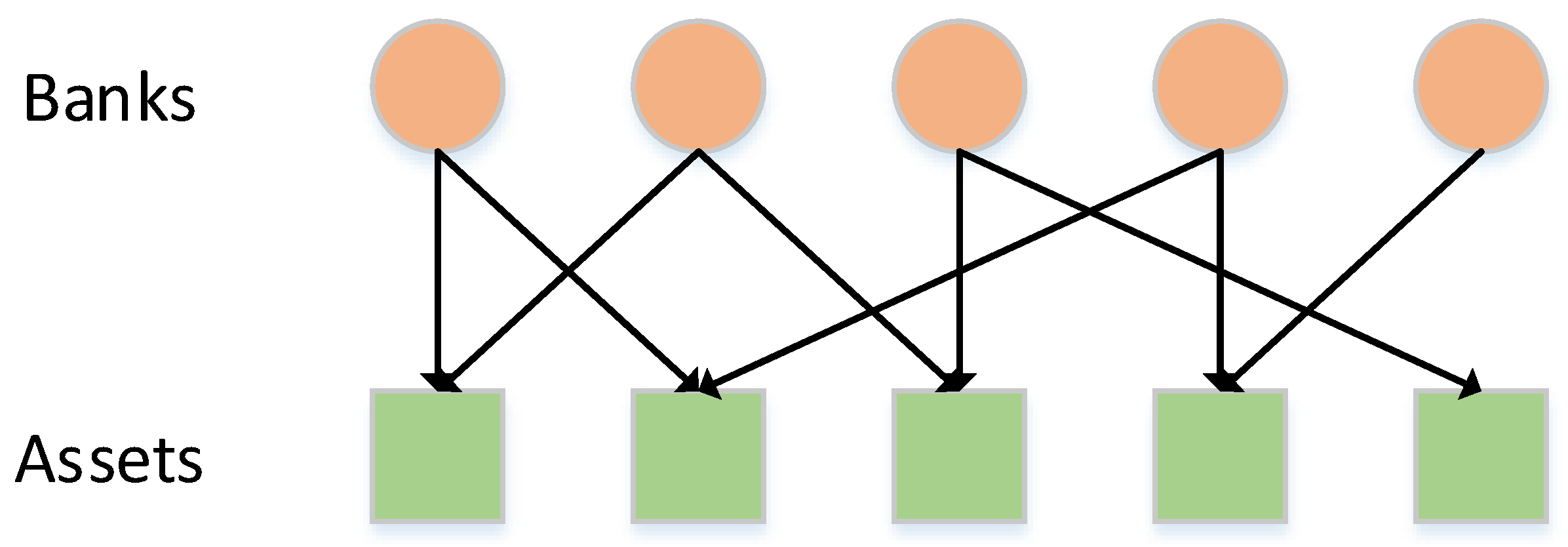
A complex network can be regarded as a set of non-empty finite point V and a binary relation E, where E refers to the edge set formed by the specific relationship between nodes. For a bank–asset bipartite network model, commercial banks and assets are regarded as 2 groups of nodes with different properties. The directional connection represents the relationship between banks holding assets. As shown in Figure 1, if commercial bank i holds asset j, a link from bank i to asset j is generated.
When establishing complex networks of real systems, we take the proportion of asset investment as the weight of the edges. First, we establish a matrix , in which the element represents the value of the asset j held by bank i. Then, we divide each by the sum of the elements in the i-th row in matrix A and derive a quantity . represents the percentage of the total value of each asset held by the bank i. After that, we establish an investment matrix E, whose -th entry equals and where the sum of the elements in each row of E is equal to 1. The element is used to represent the weight of the edge between bank node i and asset node j. According to matrix E, the bank–asset bipartite network model can be constructed. For the bipartite network, the edges are directional and only exist between bank nodes and asset nodes. Since the two group nodes can be effectively connected, the relationship between the banks and the assets in the financial system can be displayed more truly and intuitively.
2.2. A Bank Correlation Network Model
Based on a bank–asset bipartite network, we construct connected edges among banks based on the correlation of all banks’ investment portfolios and establish a connected network model among banks [23]. For any 2 bank nodes i and j, we calculate the correlation coefficient of their investment portfolio vector and obtain the correlation coefficient matrix:
where . The value of is close to 1, indicating a strong positive correlation between two bank nodes’ investment portfolios; conversely, a value close to −1 indicates a strong negative correlation. In order to avoid the negative weight of the connected edges in the network, we refer to the work of Mantegna (1999) [10] and convert the correlation coefficient to the distance value , whose calculation formula is as follows:
where . At this point, the relationship between and is monotonically decreasing. In order to ensure that the correlation coefficient and the weight of the edge change in the same direction, we introduce another formula as follows:
According to this formula, we obtain the final weight matrix . By combining this with the set of nodes, the bank correlation network can be constructed. The correlation network is a weighted and undirected network. Furthermore, since there is a correlation-based connection between any two banks, the network is a complete network model.
2.3. Community Division and Louvain Algorithm
Newman et al. (2003) defined a quantity called modularity to measure the quality of community structure [24]. Modularity refers to the ratio of edges in the community to all edges in the network minus the expected value of such a ratio when the degree of all nodes in the network remains the same but the connections are uniformly randomly generated. The formula of modularity is as follows:
where m represents the sum of the weights of all edges in the network, represents the sum of the weights of all edges of node i, represents the weight of the edges between node i and node j, and and represent the community including node i and j. The function indicates whether node i and node j are in the same community. If they are in the same community, ; otherwise, it is . The module Q can reflect the closeness of the nodes within the community, and its value range is [0, 1]. The larger the value of Q is, the closer the community is.
Based on the concept of modularity, Vincent et al. (2008) proposed a fast community division algorithm, the Louvain algorithm [25], which can accelerate the running time and rapid convergence of a community merger. The idea of the algorithm is: first, each node is regarded as an independent community. At this time, the number of communities is the same as the number of nodes. Then, we allocate node i to the communities where its neighbor nodes are located in turn and calculate the modular change after the allocation. The neighbor node with the largest value of is recorded as k. If the largest value of is greater than 0, then we allocate node i to the community where that neighbor node is located; otherwise, it remains unchanged. We repeat this process until the community structure to which all nodes belong is no longer changed, then the first iteration ends. In the process, the formula for calculating when moving an isolated node i to a community C is as follows:
where is the sum of the weights of the edges inside the community C, is the sum of the weights of the edges incident to nodes in C, is the sum of the weights of the edges incident to node i, represents the sum of the weights of the edges from i to the nodes in community C, and m represents the sum of the weights of all the edges in the network.
At the end of the first-stage iteration, the local modularity will reach its maximum value. Then, the second stage is opened, and all the nodes in the same community are regarded as a new node. This new node will have a closed loop pointing to itself, whose weight is sum of the weights of the edges in the community. The weight of the edges between any two new nodes is the sum of the weights of all the edges between the two communities. Then, we repeat the process of the first-stage iteration until the modularity of the entire network is no longer changed and the community structure is divided.
In addition, Renaud Lambiote (2003) introduced a parameter called “Resolution” to flexibly control the number and size of community division [26]. The resolution parameter can enlarge and reduce the number and scale of the community so as to realize the community division under different resolution levels and help to find the appropriate resolution level. When the resolution parameter approaches 1, the division is rough, the community scale is large, and the number of communities is small. When the resolution parameter approaches 0, the division is refined, the community scale is small, and the number of communities is large.
2.4. Nodes Importance and PageRank Algorithm
A node’s importance reflects the importance of the node in the network. There are many methods to measure the importance of nodes, such as node centrality, K-shell decomposition, the PageRank algorithm, and the LeaderRank algorithm [27]. We will apply the PageRank algorithm [28] developed by Lawrence Page to rank the importance of nodes, which has both speed and accuracy. The PageRank algorithm was originally developed to rank web pages by importance, and its basic assumption is that: (1) if a web page can be linked by many other web pages, the importance of the web page is higher; (2) if a highly important page links to another page, the importance of the page being linked to will also increase. The PageRank algorithm initially assigns the same importance score to each page, then designs an iterative algorithm based on these two assumptions to calculate the updated importance score of each page until the score is stable. The PageRank algorithm can be applied to any entity set that has the characteristic of mutual reference, and it is also suitable for ranking the importance of the nodes in a complex network. The PageRank value (PR) of node i can be expressed as follows:
where is the PageRank value of the node i to be evaluated, is the damping factor, and can be understood as the probability of a random jump to other nodes. Generally, , represents the collection of all nodes pointing to node i, and represents the sum of the weights of node j pointing to other nodes. The value is closely related to the in-degree of the node, and when the in-degree of a node is large, the value of that node tends to be larger.
Some studies show that, in a real network, the degree of most nodes is often very low and a few nodes will have a higher degree (these are called the central nodes). Only these central nodes can have a strong impact on other nodes. For many nodes, their connection path to the central nodes may be quite long, so the influence of the central nodes on them may be slow. To find out which other nodes will affect these nodes faster and more directly, the communities in which these nodes are located should also be explored, and their status in the community and their connections with other nodes should be judged. Therefore, the risk of a node is also most likely to be related to the community in which it is affected, which gives us a certain theoretical basis for studying the financial systemic risk from the perspective of community.
Since there are many methods of community division and the result of the division is not unique, it is necessary for us to use certain methods to test the reliability of the obtained community division result. In our previous paper [29], we used the Lovain algorithm to divide the communities of several types of networks with typical structures and analyzed the importance of nodes in the community sub-network. The results obtained show that there are obvious differences in the importance of nodes between different communities, and the importance ranking of all nodes in a community sub-network is highly consistent with their importance ranking in the original network, which fully demonstrates the significant effect of the community division. Based on this, we will first test the effectiveness of community structure division on bank correlation networks through the analysis of nodes importance, further analyze the differences in systemic risk between different community networks, and then explore the general law of financial systemic risk and community structure.
3. Results
3.1. Data Processing and Network Modeling
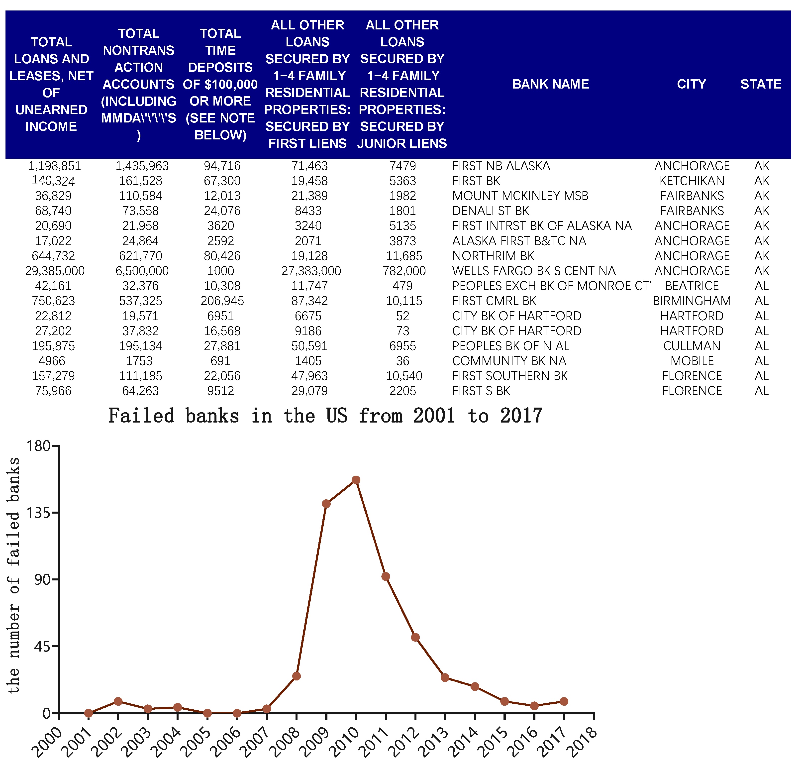
Considering the financial crisis of the U.S. in 2008, we used the U.S. commercial banks’ balance sheet data from 31 December 2007, compiled by Wharton Business School. (Data sources: https://wrds-web.wharton.upenn.edu/wrds/, accessed on 25 April 2021). The table contains the asset data of all commercial banks in 50 states of the United States, which are recorded on a quarterly basis. Some of the original data are shown in the top panel of Figure 2. In addition, we also collected the failure data of all commercial banks in 50 states of the United States from 2001 to 2017. (Data sources: http://www.fdic.gov/bank/individual/failed/banklist.html, accessed on 25 April 2021). A diagram was drawn based on the data of failed banks from 2001 to 2017, as shown in the bottom panel of Figure 2. Huang et al. (2013) elected the data from 2008 to July 2011 to examine the risk contagion of the 2008 financial crisis [30]. Combined with the overall changes in the number of failed banks since 2001, it is obvious that the number of banks failing after 2013 is quite small. Therefore, we can basically conclude that the main reason for bank failures after 2013 was not the impact of the 2008 financial crisis.
All the data in the balance sheet of U.S. banks are grouped according to the state where the bank is located. Extracting the data on 31 December 2007, we can first establish a bank–asset bilateral investment network for each state, forming 50 networks. (The data on 31 December 2007, were chosen based on the fact that the number of banks failing between 2008 and 2013 was extremely large, which can be attributed to the risk contagion caused by the 2008 financial crisis. Thus, it is necessary to establish networks close to the time when many of the banks failed, as that is when the risk contagion begins). In the balance sheet, the type of investment assets of each bank has nearly 100 indicators. However, the data on asset refinement for a large number of banks are missing. In these cases, we summarized the total assets into six types (actually, the price fluctuations of many assets will have a certain correlation. It is reasonable to regard common assets held by banks as one type of asset if they are highly correlated. Furthermore, if the asset division is too fine, the heterogeneity among banks will be quite strong and the correlation according to the investment portfolios among banks will be quite small, which will cause the weights of the edges in the bank correlation network to be small. In this case, the connection tightness among nodes in the network will be very low, which is not a positive situation for our research on the community division of the bank correlation network), which are cash in hand + reserves + loans + fixed assets + securities + other assets. Reserves include allowances for loan lease losses and allocated transfer risk reserves. Loans include real estate mortgage loans, agricultural loans, commercial and industrial loans, loans to individuals, and all other loans. Fixed assets include intangible assets, premises and fixed assets (including capitalized lease), and the total assets held in the trading account. Securities are the market value of the total investment securities. The value of other assets is calculated as the total assets minus all the other five types of assets. For a few banks, the data on securities are sometimes missing. In this case, our treatment is to set the value of other assets as 0, while the security is the total assets minus the value of the other five assets.
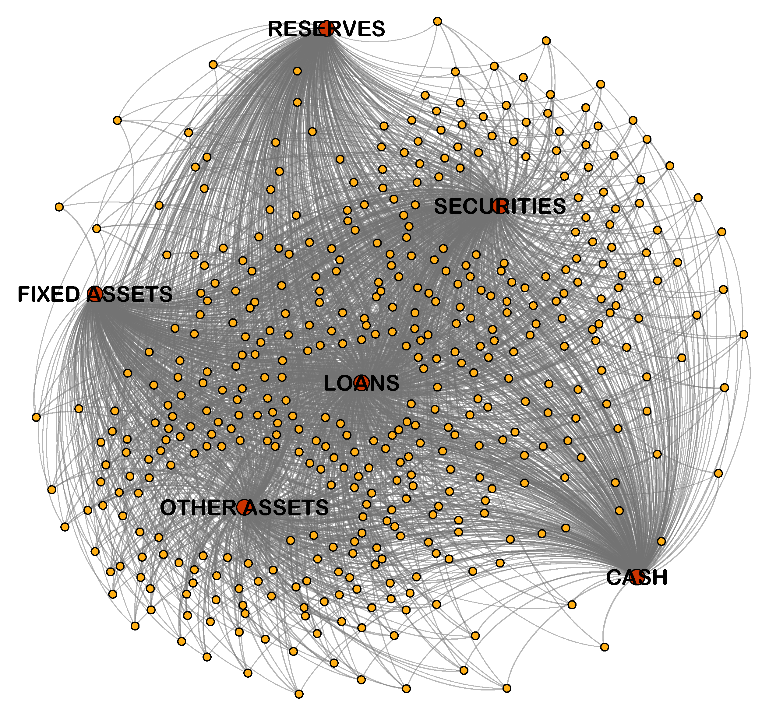
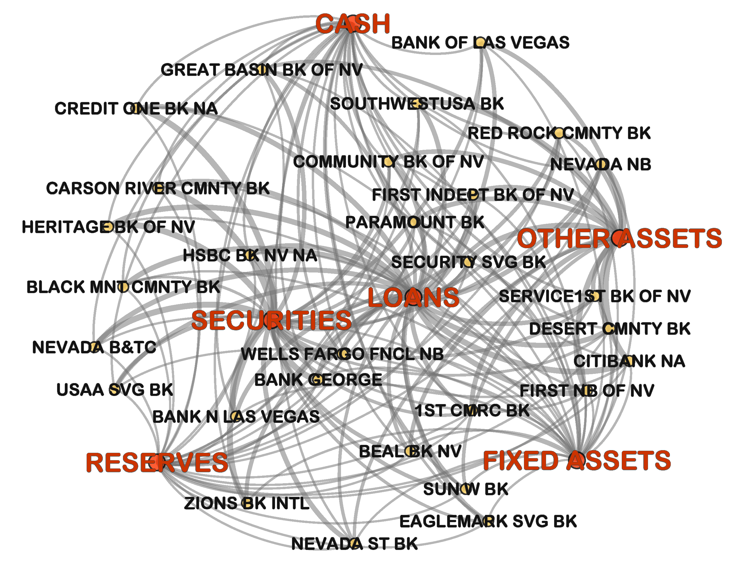
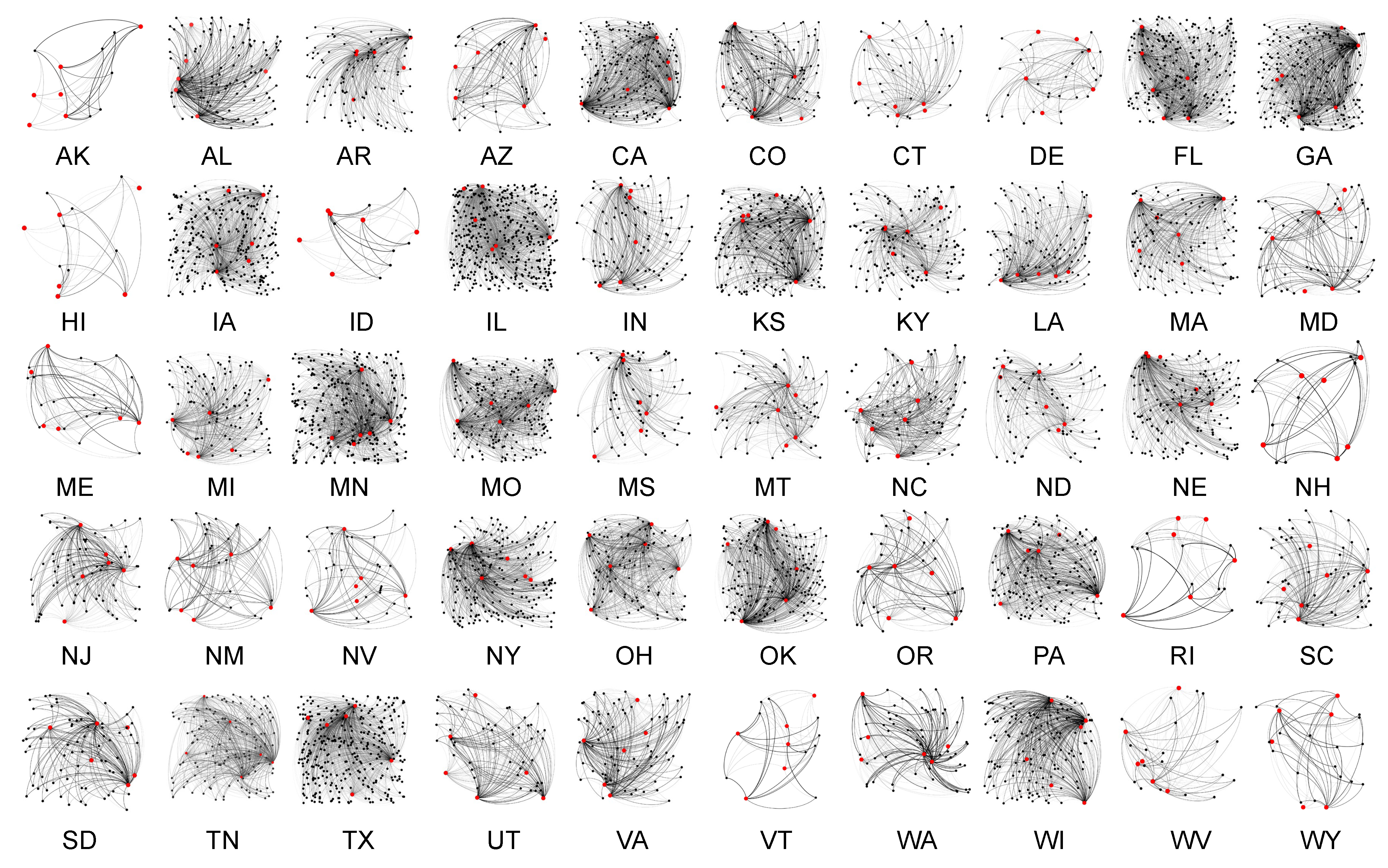
According to the above asset division, we can calculate the investment matrix E of each state on 31 December 2007, (see Section 2.2), thereby constructing a bank–asset bilateral network of each state, as shown in Figure 3. This figure shows the bank–asset bilateral networks of Illinois (IL) and Nevada (NV) on 31 December 2007. In the figure, the yellow nodes represent banks and the orange nodes represent the six types of assets, including loans, fixed assets, cash in hand, securities, reserves, and other assets. Moreover, the weight of each edge is the ratio of the investment of the asset node to the total assets of the bank node. Furthermore, the bank–asset bilateral networks of all the other states are shown in Figure 4. These figures were all created using the Gephi software. From these figures, it is obvious which states have more banks and which ones have fewer banks.
3.2. Analysis of Bank Correlation Network Model
Based on each established bank–asset bilateral network, a bank correlation network of each state can be further established. Next, we will carry out a community division and analysis of the relevant community structure of the bank correlation networks.
3.2.1. Community Division and Nodes Importance Analysis
We focused on a comparative study of states with a large number of banks, including Texas (TX), Minnesota (MN), Missouri (MO), Iowa (IA), and Illinois (IL). First, the Louvain algorithm was used to divide the five correlation networks into communities, and the resolution parameter of the division was set to 1.0 by default. Then, the PageRank algorithm was used to quantify the importance of all nodes, and scatter diagrams of the PR (PageRank) values of all the nodes in different communities were drawn for five networks, which are shown in Figure 5. The figure shows that the most important several nodes always tend to be clustered in the same community. Furthermore, we performed a statistical analysis of the PR values of the nodes in each community, as shown in Figure 5. The results are shown in Table 1, which shows that the distribution of node importance between different communities is obviously different. All the phenomena show the significance of the community division method for the bank correlation networks.
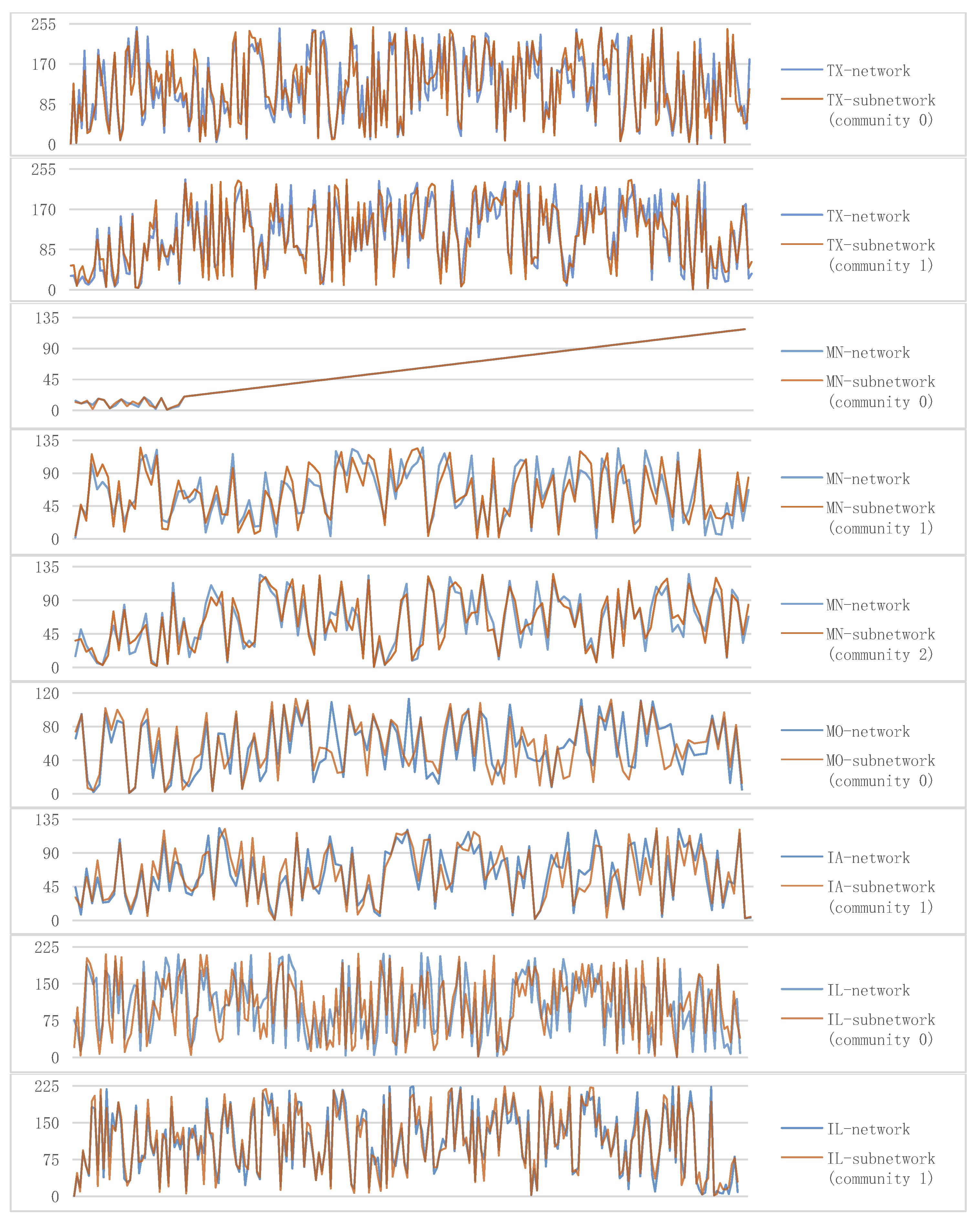
Furthermore, for each divided community, we retained the nodes and connecting edges inside this community and removed the nodes outside this community and the connections between this community and other communities to form an independent community sub-network. Then, the new PR values of these nodes in the sub-network were recalculated. The new PR value ranking of these nodes in the sub-network was compared with their PR value ranking in the original network. All the comparison results are shown in Figure 6. It can be seen that, for a group of nodes in the same community, their new PR value rank in the sub-network is highly consistent with the rank of the PR value of this group of nodes in the original network. Therefore, it can be asserted that the order trend of the two groups of PR values has a high similarity. Based on that a node’s importance reflects the important position of the node in the network and the degree of its influence on the other nodes, Figure 6 shows that, after the community division of a bank correlation network, removing the edges between communities will have little impact on the interaction between the nodes within a community. Namely, the connections between communities have little effect on the interactions between nodes within communities. Thus, after the community division, each community can basically retain the nature of these nodes in the original network.
Through the community division, some nodes that are closely connected can be divided into the same community, while the connection between two communities is lower. For a bank correlation network, nodes in the same community mean that these banks have very similar asset portfolio ratios, while the bank investment allocations between different communities are quite different. Moreover, the node importance is a very important structural characteristic of a network. A bank node with a stronger importance means that the bank has a similar asset portfolio ratio, with a greater number of banks. The different distributions of node importance among different communities show that the network structure of different communities varies greatly. The physical characteristics of the network, including systemic risk, are often determined by its basic structure. It is the great difference in node importance in different communities that provides a certain basis for us to study systemic risk from the perspective of community division. For a community sub-network, the rank of node importance is consistent with the rank of the node importance of these nodes in the original network, showing that community division does not affect the mutual relationship of nodes in a community, and the nature of the nodes in the original network can be preserved roughly. These characteristics of community division ensure the reliability of our research.
3.2.2. Community Division and Systemic Risk
Now, we focus on studying the relationship between the community sub-network structure and systemic risk of the bank correlation networks. The systemic risk is measured by the proportion of bank failures in a network from 2008 to 2013. The previous community division was carried out under the default resolution parameter of 1.0. If the resolution parameter is smaller, the division level is deeper and the number of communities obtained is larger. In this section, we set the resolution parameter to a range of [0.6, 1.0] for the network and take the values at 0.05 intervals for community division. If we take IL, with the greatest risk of bankruptcy, as an example and calculate the proportion of bankruptcies in each community under different resolution parameters, we can obtain the results shown in Figure 7. For the bank correlation network of IL, when the resolution of community division is set to be 1.0 the systemic risk of the two communities is 0.084906 and 0.084071, which means that the rough community division does not significantly distinguish the number of failed banks; if the resolution parameter is set to be 0.85, the community with the highest systemic risk reaches 0.3333, while the average risk of other communities is only 0.0607. Thus, the community division with a resolution parameter of 0.85 is more effective in distinguishing communities with higher systemic risk than that with a resolution parameter of 1.0, and this uncovers some nodes with higher risk possibilities. Bringing attention to such communities will help us to effectively supervise and control the systemic risk of the financial system.
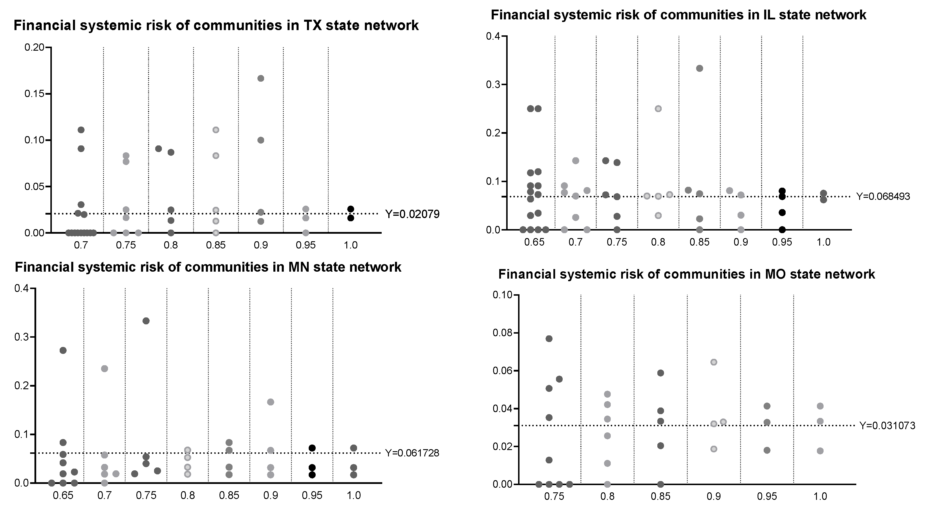
Then, we carried out community division for the bank correlation networks of TX, IL, MN, and MO states, which have a larger number of banks. The resolution parameter range was also [0.6, 1.0], and its value was taken at intervals of 0.05. The results are shown in Figure 8, where the horizontal coordinate is the resolution value and the vertical coordinate is the failure ratio of the community—namely, the systemic risk of the community. The horizontal dotted line is the entire failure ratio of the state. It can be seen that the overall systemic risks of different states vary significantly. In addition, for the same resolution, the systemic risks of different communities are quite different. Taking MN state as an example, only one of the three communities obtained under the resolution parameter of 1.0 has a higher systemic risk than the overall systemic risk value. After the resolution parameter gradually decreases, the number of communities whose systemic risk is higher than the overall systemic risk value gradually increases, and the systemic risks of different communities become more different.
Therefore, a more detailed community division may lead to significant differences in systemic risk between communities. These conclusions show that deep community divisions can effectively divide high-risk and low-risk communities.
4. Discussion
In this section, we will first examine the robustness of the community division results in the previous section. Then, we will further analyze the relationship between the sub-network structure obtained by the community division and systemic risk.
4.1. Robustness of Community Division
We used the Louvain algorithm to perform the community division of bank correlation networks. The realization of the Louvain algorithm was also based on the idea of modularity proposed by Newman et al. (2003) [24]. It is acknowledged that modularity may suffer from a resolution limit when the number of links increases. Although bank correlation networks are weighted networks and the resolution limit is less preponderant, it is necessary to test the robustness of the results of our community division. Next, we take the network of IL as an example and check the robustness of the community division results when the resolution parameter is 0.8 by retaining only the subset of links with statistically significant correlations in the bank correlation network of IL.
As for how to calculate the statistical correlation of edges, the work of Bongiorno et al. [31] gives us some inspiration. In this work, a weighted projected network is established based on a bipartite network. Then, some edges are deleted from the projected network based on some of the connection characteristics of the bipartite network itself, resulting in a statistically correct network. Since a bank correlation network is also established from the bank–asset network, it is similar to the projected network. However, the bipartite network in Bongiorno et al. is an unweighted network and just considers whether there is a connection between two nodes, while the bank–asset bipartite network we study is a weighted and nearly fully connected network that each bank invested in almost all six types of assets. Thus, the approach we take is to simply remove some edges in the bank correlation network whose weights are too small and at the same time ensure that these is at least one edge for any node. In this way, through simple calculation, we find that 25.79% of the edges with a small weight will be deleted and the remaining 74.21% edges can be retained in the bank correlation network of IL, thus obtaining a new bank association network.
Now, we will compare the community division of the new bank correlation network when the resolution parameter is set to a default of 1 with the previous community division of the IL network when the resolution parameter is 0.8. The work [31] proposed some widely used indicators to compare the accuracy and precision of the detection of pairs of nodes in a given partition. The Rand index is essentially the accuracy of the pair classification and is defined as:
In the formula, TP is the number of true positive pairs, which represents the number of pairs of nodes in the same community both in the considered and reference division. FP is the number of false positive pairs, which represents the number of pairs of nodes in the same community in the considered partition but in different communities in the reference division. (TN) is the number of true negative pairs, which represents the number of pairs when each node of the pair does not belong to the same community both in the considered division and in the reference division. Lastly, FN is the number of false negative pairs, which represents the number of pairs when each node of the pair does not belong to the same community in the considered partition while both nodes belong to the same community in the reference division. Furthermore, there is a adjusted Rand index (ARI), which is defined as
where is the expected value of the true pair classifications estimated between a random partition and the reference partition.
The precision of the pairwise classification is defined as
and an adjusted version of the index is
where
Based on these indicators, we first apply the Louvain algorithm several times by using a different initializing node sequence. Then, the output is stochastic and a different community division can be obtained. The average values of these indicators is
The results of ARI are less than desirable, which may due to the fact that the bank correlation network is a fully connected network. Nevertheless, from the results of the quantities and , the robustness of community division is quite satisfactory. Thus, the community division of the bank correlation network by the Louvain algorithm under different resolution parameters is statistically highly precise.
4.2. Relationship between Systemic Risk and Community
According to the results in Figure 8, we drew a scatter diagram of the number of community nodes and the systemic risk of the community, which is shown in Figure 9. It can be seen from Figure 9 that for these four states, communities with extremely high systemic risk often contain fewer banks. With the increase in community size, the fluctuation of systemic risk gradually decreases and is finally distributed around the value of the overall failure rate (see the horizontal dotted line in the figure).
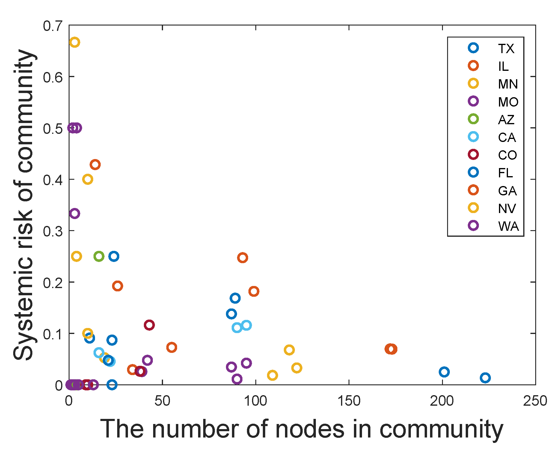
Moreover, in addition to the states TX, IL, MN, and MO, we also considered seven states with a high bank failure rate—Arizona (AZ), California (CA), Colorado (CO), Florida (FL), Georgia (GA), Nevada (NV), and Washington (WA)—and carried out the community division of the correlation networks of these states with a resolution of 0.8, resulting in a total of 69 communities. The number of nodes in these communities and the systemic risk of these communities were analyzed, and the results are plotted in Figure 10. It can be seen from this figure that, for small-scale community sub-networks, systemic risk may be extremely high or extremely low, with a wide range of values, and the sub-network is quite likely to suffer from high systemic risk. Meanwhile, for large-scale community sub-networks, the systemic risks of different communities are relatively close to a low level with a relatively narrow range of values, and the community is not prone to suffer from particularly high systemic risk.
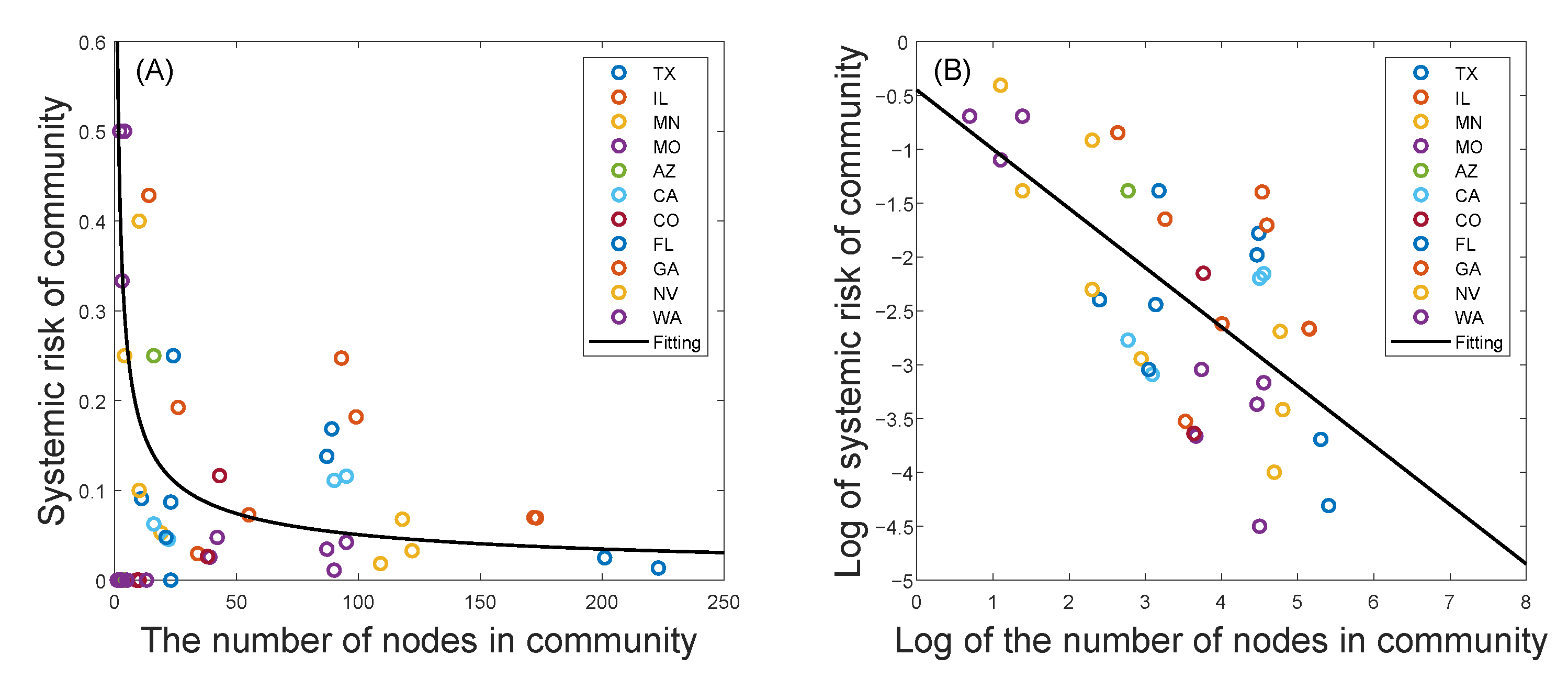
In order to deeply study the dependence of systemic risks on the size of community sub-networks, we carried out a regression analysis. According to the changing law of the nodes in Figure 10, we performed a power law distribution regression analysis on all the nodes, and the model was . Considering that the dependent variable in the model will not be equal to 0, we excluded 19 points in Figure 10 with a systemic risk value of 0 and left 50 sample points to perform the regression analysis. The results of the model are as follows:
where n represents the number of nodes in a community, represents the systemic risk of the community, and a and b are the coefficients of the model. If we take the logarithm of both sides of the model, a linear model can be obtained:
At this point, we take logarithms of the horizontal and vertical values of the points in Figure 10. The linear regression analysis result gives and , then the model is as follows:
The significant levels of and b are 0.067 and 0.000, respectively, showing that the regression effect is quite significant. With , we can derive in the original power law model. The scatter plot of the nodes in Figure 10 and the function curve of the original power law distribution are both depicted in Figure 11A. If the horizontal and vertical values of the points in Figure 10 are all logarithmic values, the function curve of the linear regression analysis function is shown in Figure 11B.
Because the community samples with systemic risk to be 0 are removed in the regression analysis, the power law distribution model can only reflect the results when the community sub-network is at risk. This is to say that, when there are certain risks in the community sub-network, the systemic risk and the size of the community show a roughly decreasing trend. Furthermore, from the characteristics of the power law distribution function, when the community size increases from a small value the systemic risk will drop sharply at the beginning, then the downward trend will gradually slow down until it is close to a small stable value. This result is consistent with the phenomenon that the financial network is “Too Big to Fail” in previous studies.
In reality, for small-scale communities, due to the small number of banks, when the network is subject to external shocks, these banks may face great risks, resulting in a sharp rise in systemic risk. It is also possible that none of these banks are affected by the external shocks and the systemic risk in this community is very low or even zero. Thus, the supervision of small-scale communities must be more vigilant due to their high probability of suffering extreme high systemic risk. Large-scale communities are usually more closely connected, and risks are diversified along the value investment relationship. Therefore, these communities may have better anti-risk ability in the face of external shocks; thus systemic risk in such communities varies little, and systemic risk will tend to be stable and be maintained at a low level.
5. Conclusions
This paper studies the systemic risks of real financial networks based on the division of community structure. In a large-scale real financial network, the use of the community division method to analyze and monitor a community sub-network can effectively simplify the network model and allow for the exploration of the potential laws of the network, which plays an important role in the study of financial network systemic risk.
Firstly, based on the investment portfolio data of all commercial banks in the United States in 2008, the correlation between banks is calculated, a correlation network model of commercial banks in each state is constructed, and the community structure of each correlation network is divided. The distribution of node importance among different communities is obviously different. Moreover, for a community sub-network, the importance ranking of all nodes in a community sub-network is highly consistent with their ranking in the original network, which verifies the effectiveness of community division for the bank correlation network established in this paper. In addition, the robustness of the community division results is tested by extracting a portion of statistically significant edges from the bank correlation network.
Then, we use the proportion of bank failures from 2008 to 2013 to measure the systemic risk and found that, for small communities, the financial systemic risk will appear to have obvious volatility. Specifically, systemic risk may be quite large or quite small, and the range of possible systemic risk is very wide. Meanwhile, there is an extremely high probability that the systemic risk of a small-scale community will be quite large. With the number of nodes in the community increasing, the systemic risk will tend towards a stable and low level. However, if only communities with failed bank are considered, the systemic risk will gradually decrease with the increase in community size, which almost conforms to the law of power law distribution. Therefore, the application of community structure division can help to identify communities with high financial systemic risk, thereby reducing the scope of network supervision from a whole network to a community sub-network, which plays a guiding role in maintaining the stability of the financial system and controlling the risk of the financial system.
In the future, it will be valuable to obtain, if possible, more actual data on bank liabilities or interbank interconnections to carry out more in-depth research and analysis. Besides this, we will further investigate the order of bank failures, analyze the type of communities in which they are located, and try to obtain the latest data to analyze the dynamic behavior of the network and assess the change in systemic risk over time. In addition, differences in actual conditions such as industry and national conditions will lead to the existence of many types of networks with different topology characteristics. In the follow-up study, the applicability of our research method in more different types of networks will be further discussed.
Author Contributions
Conceptualization, Y.H.; methodology, Y.H.; software, F.C.; validation, Y.H. and F.C.; formal analysis, Y.H. and F.C.; investigation, F.C.; resources, Y.H.; data curation, F.C.; writing—original draft preparation, F.C.; writing—review and editing, Y.H.; visualization, Y.H.; supervision, Y.H.; project administration, Y.H.; funding acquisition, Y.H. All authors have read and agreed to the published version of the manuscript.
Funding
The contribution to this research by Y.H. was supported by the Fundamental Research Funds for the Central Universities (Grant no. BLX201722).
Institutional Review Board Statement
Not applicable.
Informed Consent Statement
Not applicable.
Data Availability Statement
Publicly available datasets were analyzed in this study. These data can be found on the website: https://wrds-web.wharton.upenn.edu/wrds/ and http://www.fdic.gov/bank/individual/failed/banklist.html (accessed on 1 April 2021).
Acknowledgments
This work was supported by the Fundamental Research Funds for the Central Universities (Grant no. BLX201722).
Conflicts of Interest
The authors declare that they have no conflict of interest to report regarding the present study.
References
- Elliott, M.; Golub, B.; Jackson, M.O. Financial networks and contagion. Am. Econ. Rev. 2014, 104, 3115–3153. [Google Scholar] [CrossRef] [Green Version]
- Hart, O.; Zingales, L. How to Avoid a New Financial Crisis; Working Paper; University of Chicago: Chicago, IL, USA, 2009. [Google Scholar]
- Brunnermeier, M.K. Deciphering the liquidity and credit crunch 2007–2008. J. Econ. Perspect. 2009, 23, 77–100. [Google Scholar] [CrossRef] [Green Version]
- Diamond, D.W.; Dybvig, P.H. Bank Runs, Deposit insurance and liquidity. J. Political Econ. 1983, 91, 401–419. [Google Scholar] [CrossRef]
- Lenzu, S.; Tedeschi, G. Systemic risk on different interbank network topologies. Phys. A Stat. Mech. Appl. 2012, 391, 4331–4341. [Google Scholar] [CrossRef] [Green Version]
- Chinazzi, M.; Fagiolo, G. Systemic Risk, Contagion, and Financial Networks: A Survey; Institute of Economics, Scuola Superiore Sant’Anna, Laboratory of Economics and Management (LEM): Pisa, Italy, 2015. [Google Scholar]
- Raffestin, L. Diversification and systemic risk. J. Bank. Financ. 2014, 46, 85–106. [Google Scholar] [CrossRef]
- Ma, Q.; He, J.; Li, S.; Sui, X. Investigating banking systemic risk within an endogenous network. J. Dalian Univ. Technol. (Soc. Sci.) 2018, 39, 32–39. [Google Scholar]
- Yang, H.F.; Liu, C.L.; Chou, R.Y. Bank diversification and systemic risk. Q. Rev. Econ. Financ. 2020, 77, 311–326. [Google Scholar] [CrossRef]
- Mantegna, R.N. Hierarchical structure in financial markets. Eur. Phys. J. B-Condens. Matter Complex Syst. 1999, 11, 193–197. [Google Scholar] [CrossRef] [Green Version]
- Onnela, J.P.; Chakraborti, A.; Kaski, K.; Kertesz, J. Dynamic asset trees and Black Monday. Phys. A Stat. Mech. Appl. 2003, 324, 247–252. [Google Scholar] [CrossRef] [Green Version]
- Brida, J.G.; Risso, W.A. Multidimensional minimal spanning tree: The Dow Jones case. Phys. A Stat. Mech. Appl. 2008, 387, 5205–5210. [Google Scholar] [CrossRef]
- Huang, W.Q.; Zhuang, X.T.; Yao, S. A network analysis of the Chinese stock market. Phys. A Stat. Mech. Appl. 2009, 388, 2956–2964. [Google Scholar] [CrossRef]
- May, R.M.; Arinaminpathy, N. Systemic risk: The dynamics of model banking systems. J. R. Soc. Interface 2010, 7, 823–838. [Google Scholar] [CrossRef]
- Beale, N.; Rand, D.G.; Battey, H.; Croxson, K.; May, R.M.; Nowak, M.A. Individual versus systemic risk and the regulator’s dilemma. Proc. Natl. Acad. Sci. USA 2011, 108, 12647–12652. [Google Scholar] [CrossRef] [Green Version]
- Glasserman, P.; Young, H.P. How likely is contagion in financial networks? J. Bank. Financ. 2015, 50, 383–399. [Google Scholar] [CrossRef] [Green Version]
- Caccioli, F.; Shrestha, M.; Moore, C.; Farmer, J.D. Stability analysis of financial contagion due to overlapping portfolios. J. Bank. Financ. 2014, 46, 233–245. [Google Scholar] [CrossRef] [Green Version]
- Fortunato, S. Community detection in graphs. Phys. Rep. 2010, 486, 75–174. [Google Scholar] [CrossRef] [Green Version]
- Derry, J.; Mangravite, L.; Suver, C.; Furia, M.; Henderson, D.; Schildwachter, X.; Izant, J.; Sieberts, S.; Kellen, M.; Friend, S. Developing predictive molecular maps of human disease through community-based modeling. Nat. Prec. 2011, 1. [Google Scholar] [CrossRef]
- Papadopoulos, S.; Kompatsiaris, Y.; Vakali, A.; Spyridonos, P. Community detection in social media. Data Min. Knowl. Discov. 2012, 24, 515–554. [Google Scholar] [CrossRef]
- Bedi, P.; Sharma, C. Community detection in social networks. Wiley Interdiscip. Rev. Data Min. Knowl. Discov. 2016, 6, 115–135. [Google Scholar] [CrossRef]
- Johnson, N.F.; Zheng, M.; Vorobyeva, Y.; Gabriel, A.; Qi, H.; Velásquez, N.; Manrique, P.; Johnson, D.; Restrepo, E.; Song, C.; et al. New online ecology of adversarial aggregates: ISIS and beyond. Science 2016, 352, 1459–1463. [Google Scholar] [CrossRef] [Green Version]
- Onnela, J.P.; Kaski, K.; Kertész, J. Clustering and information in correlation based financial networks. Eur. Phys. J. B 2004, 38, 353–362. [Google Scholar] [CrossRef]
- Newman, M.E.J.; Girvan, M. Finding and evaluating community structure in networks. Phys. Rev. E 2004, 69, 026113. [Google Scholar] [CrossRef] [PubMed] [Green Version]
- Blondel, V.D.; Guillaume, J.L.; Lambiotte, R.; Lefebvre, E. Fast unfolding of communities in large networks. J. Stat. Mech. Theory Exp. 2008, 2008, P10008. [Google Scholar] [CrossRef] [Green Version]
- Lambiotte, R. Multi-scale modularity and dynamics in complex networks. In Dynamics on and of Complex Networks; Birkhuser: New York, NY, USA, 2013; Volume 2, pp. 125–141. [Google Scholar]
- Li, Q.; Zhou, T.; Lv, L.; Chen, D. Identifying influential spreaders by weighted LeaderRank. Phys. A Stat. Mech. Its Appl. 2014, 404, 47–55. [Google Scholar] [CrossRef] [Green Version]
- Brin, S.; Page, L. The anatomy of a large-scale hypertextual Web search engine. Comput. Netw. ISDN Syst. 1998, 30, 107–117. [Google Scholar] [CrossRef]
- Chen, F.; Huang, Y. Research on the Nodes Importance in Complex Networks Based on Community Partition. In Proceedings of the 2nd International Conference on Big Data Technologies, Jinan, China, 28 August–30 August 2019; pp. 272–277. [Google Scholar]
- Huang, X.; Vodenska, I.; Havlin, S.; Stanley, H.E. Cascading failures in bi-partite graphs: Model for systemic risk propagation. Sci. Rep. 2013, 3, 1219. [Google Scholar] [CrossRef] [Green Version]
- Bongiorno, C.; London, A.; Miccichè, S.; Mantegna, R.N. Core of communities in bipartite networks. Phys. Rev. E 2017, 96, 022321. [Google Scholar] [CrossRef] [PubMed] [Green Version]
Figure 1.
A bilateral network of banks and assets.

Figure 2.
The top panel: the data of the balance sheet. The bottom panel: the number of banks that failed each year from 2001 to 2017.
Figure 2.
The top panel: the data of the balance sheet. The bottom panel: the number of banks that failed each year from 2001 to 2017.

Figure 3.
The bilateral bank–asset networks of IL (the top one) and NV (the bottom one) states. The big yellow nodes represent banks, the small orange nodes represent the six types of assets, and the thickness of each edge is proportional to its weight.
Figure 3.
The bilateral bank–asset networks of IL (the top one) and NV (the bottom one) states. The big yellow nodes represent banks, the small orange nodes represent the six types of assets, and the thickness of each edge is proportional to its weight.


Figure 4.
The bilateral bank–asset network of each state in the United States. The black nodes represent banks, the orange nodes represent the six types of assets, and the thickness of each edge is proportional to its weight.
Figure 4.
The bilateral bank–asset network of each state in the United States. The black nodes represent banks, the orange nodes represent the six types of assets, and the thickness of each edge is proportional to its weight.

Figure 5.
Scatter diagrams of PR values for communities in the five networks of TX, MO, MN, IL, and IA.
Figure 5.
Scatter diagrams of PR values for communities in the five networks of TX, MO, MN, IL, and IA.

Figure 6.
Comparison of the PR values in the original network and community sub-network of five networks.
Figure 6.
Comparison of the PR values in the original network and community sub-network of five networks.

Figure 7.
The results of the community division of the IL network with a different resolution.

Figure 8.
Comparison of the systemic risk of different communities of four networks.

Figure 9.
Relationship between systemic risk and the number of nodes in the community.

Figure 10.
Relationship between systemic risk and the number of nodes in the community when the resolution parameter is 0.8.
Figure 10.
Relationship between systemic risk and the number of nodes in the community when the resolution parameter is 0.8.

Figure 11.
The results of regression analysis on the nodes in Figure 10. (A) shows the power law distribution of points in Figure 10. (B) shows the result after taking the logarithm to the horizontal and vertical values of points in (A).


Table 1.
Statistical analysis of the PR values of nodes in each community shown in Figure 5.
Table 1.
Statistical analysis of the PR values of nodes in each community shown in Figure 5.
| Community | N | Mean of PR Values | Variance of PR Values |
|---|---|---|---|
| TX | 248 | 2.22523743548387 | 0.0215978777464978 |
| TX | 233 | 1.92335242060086 | 0.0659583239182102 |
| MO | 120 | 2.81006100453333 | 0.107091500416574 |
| MO | 121 | 2.51621886913223 | 0.0255431313667735 |
| MO | 113 | 3.17106368377876 | 0.0049496146085455 |
| MN | 118 | 2.71631342961864 | 0.0469145350950722 |
| MN | 125 | 2.624615255376 | 0.0338409023282173 |
| MN | 125 | 2.811184867392 | 0.0160391232523291 |
| IL | 212 | 2.3452891415849 | 0.0132360279522334 |
| IL | 226 | 2.22477301762389 | 0.0512349427066714 |
| IA | 122 | 3.85486265188524 | 0.0200009060100606 |
| IA | 17 | 3.31266943647059 | 0.0154961123730195 |
| IA | 123 | 3.84871037436585 | 0.130251077681873 |
a The subscripts indicate the different communities in the state’s banks correlation network. b N respresents the number of nodes in each community.
Publisher’s Note: MDPI stays neutral with regard to jurisdictional claims in published maps and institutional affiliations. |
© 2021 by the authors. Licensee MDPI, Basel, Switzerland. This article is an open access article distributed under the terms and conditions of the Creative Commons Attribution (CC BY) license (https://creativecommons.org/licenses/by/4.0/).
Share and Cite
MDPI and ACS Style
Huang, Y.; Chen, F. Community Structure and Systemic Risk of Bank Correlation Networks Based on the U.S. Financial Crisis in 2008. Algorithms 2021, 14, 162. https://0-doi-org.brum.beds.ac.uk/10.3390/a14060162
AMA Style
Huang Y, Chen F. Community Structure and Systemic Risk of Bank Correlation Networks Based on the U.S. Financial Crisis in 2008. Algorithms. 2021; 14(6):162. https://0-doi-org.brum.beds.ac.uk/10.3390/a14060162
Chicago/Turabian StyleHuang, Yajing, and Feng Chen. 2021. "Community Structure and Systemic Risk of Bank Correlation Networks Based on the U.S. Financial Crisis in 2008" Algorithms 14, no. 6: 162. https://0-doi-org.brum.beds.ac.uk/10.3390/a14060162
Note that from the first issue of 2016, this journal uses article numbers instead of page numbers. See further details here.