
Efficient and Scalable Initialization of Partitioned Coupled Simulations with preCICE


1
Institute for Parallel and Distributed Systems (IPVS), University of Stuttgart, 70569 Stuttgart, Germany
2
Scientific Computing in Computer Science, Technical University of Munich (TUM), 85748 Garching, Germany
*
Author to whom correspondence should be addressed.
Algorithms 2021, 14(6), 166; https://0-doi-org.brum.beds.ac.uk/10.3390/a14060166
Submission received: 30 April 2021
/
Revised: 22 May 2021
/
Accepted: 25 May 2021
/
Published: 27 May 2021
(This article belongs to the Special Issue High-Performance Computing Algorithms and Their Applications 2021)
Abstract
:preCICE is an open-source library, that provides comprehensive functionality to couple independent parallelized solver codes to establish a partitioned multi-physics multi-code simulation environment. For data communication between the respective executables at runtime, it implements a peer-to-peer concept, which renders the computational cost of the coupling per time step negligible compared to the typical run time of the coupled codes. To initialize the peer-to-peer coupling, the mesh partitions of the respective solvers need to be compared to determine the point-to-point communication channels between the processes of both codes. This initialization effort can become a limiting factor, if we either reach memory limits or if we have to re-initialize communication relations in every time step. In this contribution, we remove two remaining bottlenecks: (i) We base the neighborhood search between mesh entities of two solvers on a tree data structure to avoid quadratic complexity, and (ii) we replace the sequential gather-scatter comparison of both mesh partitions by a two-level approach that first compares bounding boxes around mesh partitions in a sequential manner, subsequently establishes pairwise communication between processes of the two solvers, and finally compares mesh partitions between connected processes in parallel. We show, that the two-level initialization method is fives times faster than the old one-level scheme on 24,567 CPU-cores using a mesh with 628,898 vertices. In addition, the two-level scheme is able to handle much larger computational meshes, since the central mesh communication of the one-level scheme is replaced with a fully point-to-point mesh communication scheme.
1. Introduction
Numerical methods to solve multi-physics problems can be generally categorized into two groups, monolithic and partitioned. In a monolithic approach, all governing equations from different domains are discretized and solved as a single large system. On the other hand, in a partitioned approach, the problem is divided into different sub-domains according to the occurring physics. As a result, this method employs separate solvers for various sub-problems and adopts a coupling technique to account for the interaction of the domains. Partitioned approaches provide the opportunity to use the most adapted and well-validated numerical methods and software for each sub-problem, which reduces the software development effort. However, this approach requires the coupling between the separate solvers. preCICE is a library designed for black-box coupling of several simulation codes. It allows to establish multi-physics multi-code simulation environments. Typical use cases of preCICE encompass fluid-structure interaction in aerodynamics [1] or blood flow simulations [2,3], interactions between free flow and flow in porous media in geoscience and environmental engineering [4], or hybrid turbulence models [5]. To realize the coupling, preCICE offers all necessary ingredients, in particular communication between parallel simulation codes [6], data mapping between non-matching discretizations [7], and iterative implicit coupling along with convergence acceleration techniques such as under-relaxation and advance quasi-Newton methods (e.g., [8,9,10]). preCICE particularly targets multi-physics simulations on high performance computers. Such parallel simulations allow for mirroring the model accuracy of sophisticated multi-physics models in corresponding high resolution of the numerical schemes. To be able to exploit large high performance computing systems, these simulations are usually parallelized for distributed memory systems by use of MPI (Message Passing Interface (https://www.mpi-forum.org/)) and partitioning of the whole simulation domain into sub-domains (partitions). In this paper, we present latest performance and scalability improvements of the coupling library preCICE.
To couple MPI-parallel codes, preCICE uses a pure peer-to-peer concept avoiding any server-like central entity. Coupling numerics (such as radial-basis function interpolation or quasi-Newton acceleration) are computed directly within the library on the processes of the coupled codes [6]. Coupling data are exchanged in a point-to-point manner between coupled codes. This makes the computational cost of the actual coupling per time step negligible compared to the typical run time of the coupled codes themselves, even for very large cases on ten thousands of processes [11]. So far, the performance of the initialization of the coupling was considered non-critical. The implementation used by Uekermann [11] still had multiple potential bottlenecks including sequential gather-scatter algorithms. For many coupled simulations, this is justifiable, since a very high number of time steps is required after a single initialization. However, the initialization can become a limiting factor, if we either reach memory limits in gather-scatter algorithms, or if we have to re-initialize communication relations due to dynamic changes in mutual data dependencies between coupled codes.
Lindner [12,13] already removed several initialization bottlenecks concerning the creation of communication channels, on the one hand, and neighborhood search between mesh partitions of two solvers, on the other hand. We briefly summarize both efforts in this and the following paragraph. preCICE offers two communication backends to realize communication between two codes: MPI and Transmission Control Protocol (TCP)/IP. In general, the coupled parallel use MPI for their internal communication. If MPI is chosen as communication backend, we create inter-communicators through MPI ports to connect the coupled codes. Previously, we had used one communicator for each interacting pair of processes. Lindner replaced this concept by only using a single communicator per coupling. This drastically reduced the cost for creation of communication channels and also improved efficiency of the actual data communication on some high-performance computing architectures. To establish TCP/IP-based connections, each pair of connected processes needs to exchange a connection token via the file system. Storing all tokens in a single directory can exert a heavy load on the file system. To reduce the load on the file system, Lindner introduced a hash-based scheme, which distributes the connection files among different directories in an optimal way reducing the file system load significantly.
Besides for establishing communication channels between processes of separate parallel solvers, mesh partitions of the two solvers have to be compared to determine exact data dependencies between mesh entities for data mapping between the two non-matching meshes. For data mapping, preCICE offers three methods: nearest-neighbor mapping, nearest-projection mapping, and radial basis function (RBF) interpolation. For all three methods, a neighborhood search of mesh vertices is required during initialization. Using a tree-based approach, Lindner reduced this cost in case of the nearest-neighbor mapping from to , assuming the coupling meshes of two coupled codes both have n vertices. Similarly, he was able to speed-up the initialization of the RBF interpolation system matrix.
In this contribution, we tackle two remaining initialization bottlenecks, which still hinder very large coupled simulations. Firstly (Section 3), we extend the tree-based approach neighbor search between mesh partitions to the more complex nearest-projection data mapping, where not only data points, but also edges and triangles interact. Secondly (Section 2), we remove gather-scatter components of the initialization. To briefly introduce the latter, let us consider the coupling of two codes A and B. To determine, which processes of A need communication channels to which processes of B, the partitions of the coupling meshes of both codes need to be compared during initialization. To this end, preCICE previously first gathered the whole coupling mesh of B at a single master process of B. Then, the mesh was sent from the master process of B to the master process of A and was broadcast afterwards to all processes of A. As a last step, each process of A reduced the received mesh of B to its required partition. For this last step, the partitioning of mesh A as well as the defined data mapping between A and B was used. We now replace this one-level gather-scatter approach by a two-level scheme. On the first level, we only use bounding boxes around mesh partitions in a gather-scatter manner to determine preliminary communication channels. On the second level, we then communicate full mesh data point-to-point and reduce the communication channels to their final set. We then can combine all ingredients, the improvements of Lindner and the contributions of this work, to a very efficient and scalable initialization (Section 4).
Similar coupling software as preCICE exist with different strategies to initialize communication and data mapping. We briefly compare these strategies to ours. The commercial tool MpCCI [14] initializes the coupling on a centralized coupling server [15], which degrades the scalability of the initialization [11]. DTK [16] creates a third rendezvous decomposition on additional coupling processors to correlate two independently decomposed meshes. To this end, a recursive coordinate bi-sectioning algorithm is used, which can completely operate on distributed mesh structures [17]. OpenPALM [18] follows a similar bounding-box approach for comparing mesh partitions as the one we propose in this contribution. Afterwards, octree-based data structures are used to accelerate the search process within each mesh partition. MUI [19] does not create mesh structures at initialization, but computes on-the-fly data mapping in every coupling step. This allows for the coupling of dynamically changing meshes and particle codes. To avoid all-to-all communication, each process can optionally define additional regions of interest, which are compared during initialization similar to our bounding-box comparison. Finally, CUPyDO [20] follows a similar approach as preCICE previously used [11]: mesh partitions are gathered and scattered by a single process during initialization.
2. Two-Level Initialization
In order to effectively address the scalability and memory issues of communication initialization in preCICE, explained in Section 1, we introduce a two-level approach. The new scheme is implemented in the preCICE library and is available starting from preCICE v2.0. The goal of the initialization phase is to identify required communication channels together with the respective data to be sent and received between the parallel processes of coupled solvers. The new scheme breaks down this process into two levels. The first level identifies and establishes potentially required communication channels, while the second level specifies the actual list of data to be exchanged.
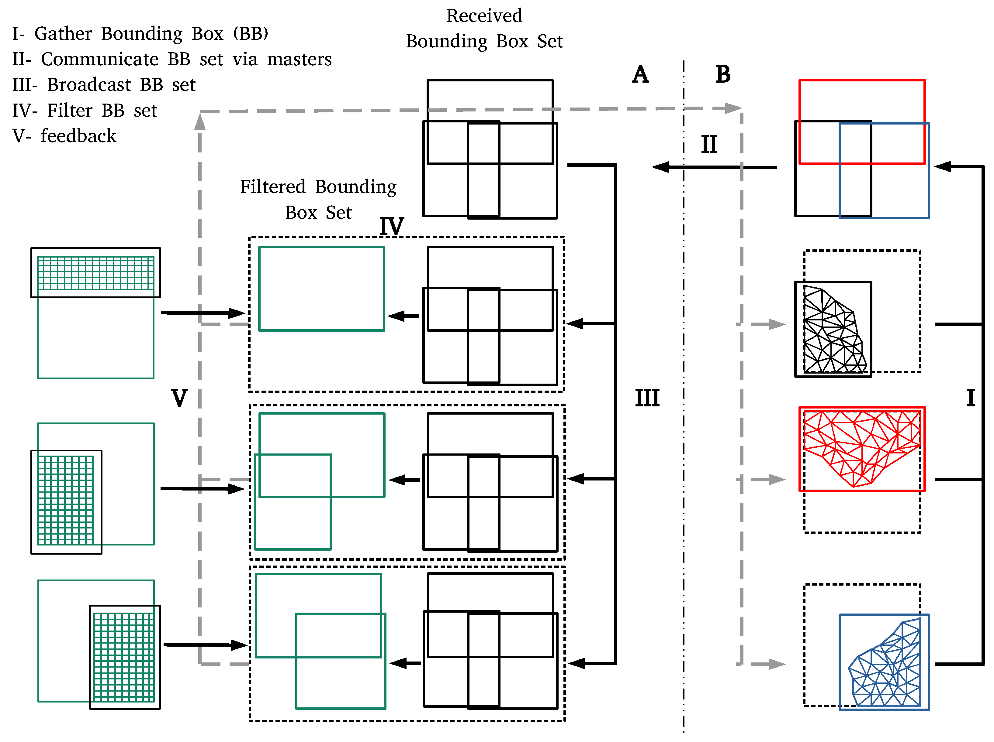
In the first level, each process located at the common interface computes a bounding box around its coupling mesh partition, see Figure 1. The bounding box is defined by the range of x-, y-, and z-coordinates of the respective mesh partition. The master process of one solver (Solver B in the example in Figure 1) gathers the bounding boxes of all processes with a non-empty coupling region (coupling processes). This corresponds to step I in Figure 1. The set of bounding boxes is communicated to the other solver via master-to-master communication and then broadcast to all coupling processes of the receiving solver (step II and III in Figure 1). Each process of the receiving solver (Solver A) compares its bounding box to the received set of boxes to identify relevant partner processes with mesh partitions that potentially interact with the own coupling mesh partition in the given data mapping (step IV). This step provides the required information regarding the list of connected processes to establish communication channels. Note, that not all pairs of processes on this list actually exchange data, but the list is already much shorter than the total number of possible pairs. preCICE uses this information to establish the communication channels. preCICE offers two options for communication channels: (i) based on MPI via MPI ports or (ii) using lower level TCP/IP sockets. For MPI-based communication, preCICE generates a single extra MPI communicator including all coupling processes of both solvers. For the TCP/IP-based communication, preCICE employs a hash-based directory and file naming scheme to store the connection tokens in an optimal distributed way. This approach reduces the load on the file system substantially. More details on creating communication channels in preCICE can be found in [12].
The presented approach eliminates the gathering of the complete coupling mesh data at the master process and the subsequent scattering at the partner solver. Thus, we remove the memory issue of our previous approach (see Section 1) and can run highly parallel high resolution simulations even if the whole coupling mesh does not fit into the memory assigned to a single process. For storing and communicating bounding boxes, preCICE uses a C++ std::map data structure, which maps the process id to its bounding box. This facilitates the bounding box set communication and filtering in the receiving partition.
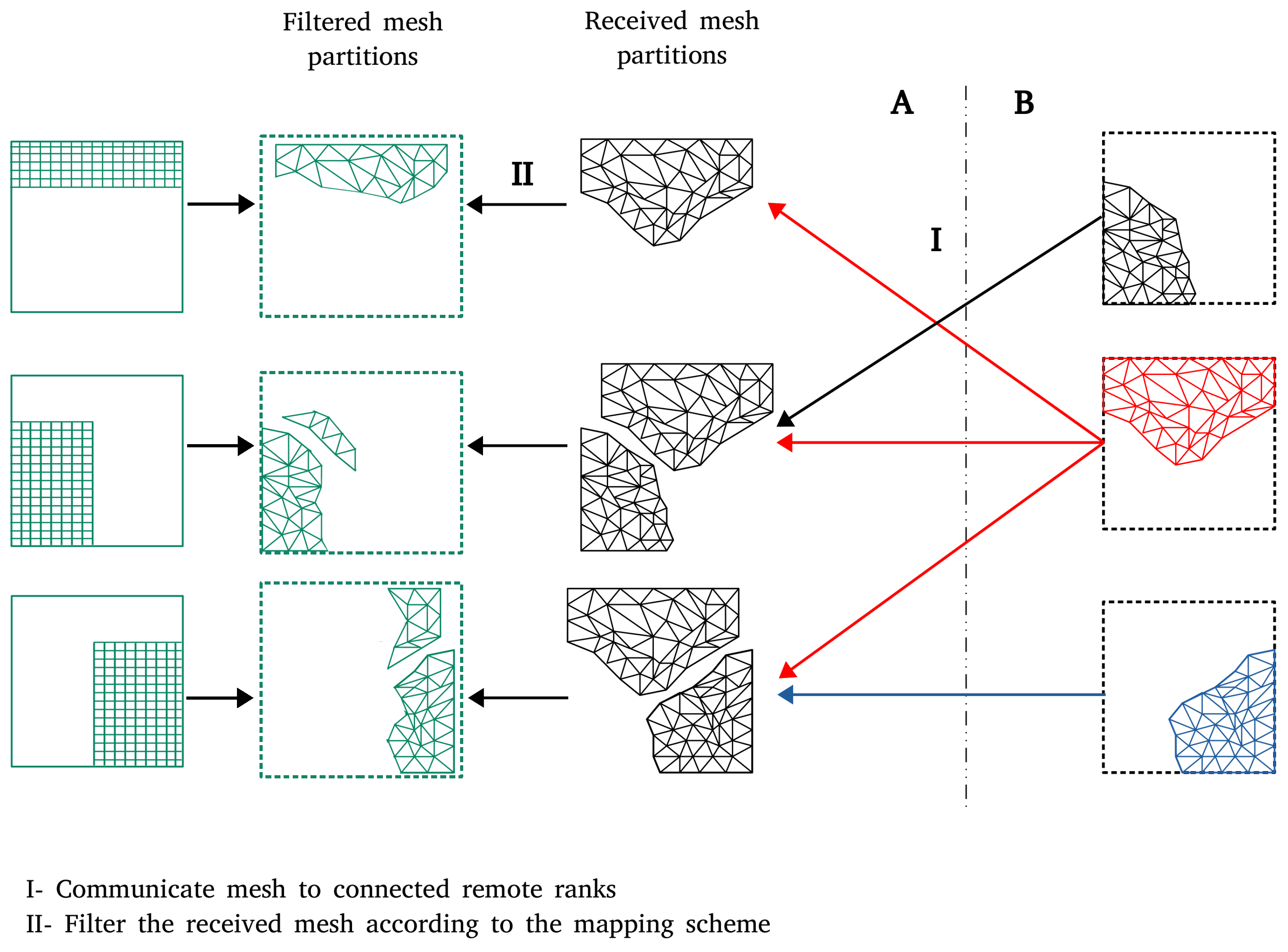
In the second level, using the point-to-point communication channels established in the first level, partner processes exchange their mesh partitions (step I in Figure 2). The processes of the receiving solver A compare their mesh partition to the received partitions to filter and identify the list of data that must be communicated during run time (step II in Figure 2). The mesh filter has to be done considering the configured data mapping scheme. The filtering process is explained in detail in Section 3. The direct mesh communication between partner processes improves the scalability of the initialization scheme since both the exchange and the filtering are executed in parallel.
3. R-Tree-Based Mesh Filtering
For the mesh filtering step (step II in Figure 2), we need to determine, which parts of the received mesh partitions are required to carry out the data mapping between both meshes, the own mesh of the receiving solver and the received mesh. preCICE supports three data mapping methods: nearest-neighbour mapping, nearest-projection mapping, and radial-basis-function interpolation. Moreover, all data mapping methods come in two flavors: consistent and conservative [21]. The required flavor depends on the type of data: Normalized quantities such as temperatures, displacements, velocities, or stresses require a consistent data mapping, while cumulative quantities such as mass or forces require a conservative data mapping. preCICE only supports consistent data mapping from the received mesh to the own mesh and conservative data mapping from the own mesh to the received mesh. If consistent (or conservative) data mapping is required in both directions, both meshes need to be communicated and repartitioned during initialization. To prepare the data mapping, we need to ’filter’ the received mesh partitions, i.e., we need to carry out a neighbor search from all data points of the own mesh partition (mesh A in Figure 2), called origin mesh in the filtering process, and data points of the received mesh partition (mesh B in Figure 2, called search mesh in the filtering process). If we assume that both mesh partitions have n data points, a naive implementation of this neighbor search requires comparisons. Each of these comparisons can involve computing a simple Euclidean distance between vertices (for nearest-neighbor mapping), but also a more complex vertex-triangle projection followed by a barycentric interpolation within the triangle (for nearest-projection mapping). Figure 3 shows 2D examples for both mappings.
In the following, we present recent improvements of spatial lookups, i.e., the identification of relevant neighbors for a single data point of the origin mesh in the search mesh for the projection-based mappings (nearest neighbor and nearest projection), which is an extension of the work presented in [12]. After introducing the used data-structure and necessary nomenclature, we briefly explain the nearest-neighbor mapping followed by the fundamentals and implementation of the nearest-projection mapping.
To accelerate spatial lookups, we use the rtree data-structure from Boost.geometry [22] with the R*-tree insertion strategy, which stores spatial data in a hierarchical data-structure. The approach for inserting data points into the tree according to the R*-tree insertion strategy aims at minimizing the area, margin, and overlap of tree nodes which leads to a good average query performance (compared to linear and quadratic R-trees) at a higher construction cost [23]. The insertion strategy can be parameterized with the maximum and minimum amount of elements per tree node, where we use the default values of Boost.geometry (16 and ) similarly to [12]. The R*-tree and the R-tree have the same complexities: an insertion complexity of and a query complexity of for n spatially distributed data points [24]. As, in general, meshes are immutable in preCICE, we choose the R*-tree as the higher construction cost pays off in terms of improved lookup performance. The Boost.geometry data structure provides k-nearest-neighbor queries, which the nearest-neighbor mapping and the nearest-projection mapping require, in . The data structure also allows for bounding box queries, which the radial-basis-function mapping requires, in .
Let the dimension d be 2 or 3. The search mesh has a vertex set and a mesh connectivity information given by an edge set with size and a triangle set with size for . We further use . The origin mesh has a vertex set . Nearest-neighbor mapping and radial-basis-function mapping operate on vertices only. Thus, it is beneficial to store each set of primitives of the search mesh (, , ) in a separate index tree to avoid overhead.
A nearest-neighbor data mapping searches for the nearest vertex in for each vertex of . This requires to insert all vertices of into the R-tree resulting in a complexity of . Afterwards, we query for the nearest-neighbor of each vertex of at a total cost of .
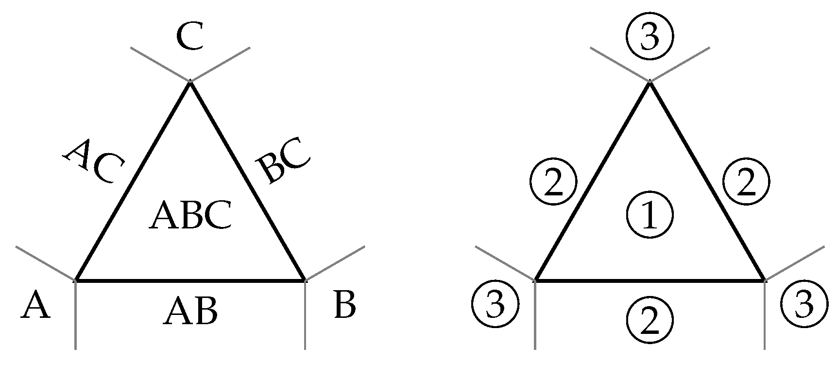
A nearest-projection data mapping searches for the nearest primitive (vertex, edge, or triangle) of for each vertex of . We use a cascading scheme: For (see Figure 4), the mapping attempts to first find an orthogonal projection onto a triangle, if this fails, it tries to compute an orthogonal projection onto an edge, and finally, if this also fails, selects the closest vertex. For , the above method starts at projecting onto an edge.
For a more precise description, let us categorize primitives by their degree: for vertices, edges, and triangles, respectively. Then, a nearest projection of degree 1 of a vertex is simply a nearest-neighbor search. More interestingly, to find the nearest projection of degree or of ,
- we fetch the k nearest primitives of degree m of vertex ,
- we sort them by ascending distance to ,
- we process the list of primitives and calculate interpolation weights for data interpolation from the primitive’s vertices to the projection point on the respective plain or line,we terminate and return the current primitive, if all weights are positive ,
- we return the nearest projection of degree of vertex u if no valid projection of degree m could be found.
This cascading scheme requires to probe all primitives and, thus, to index the complete search mesh in an R-tree. This is of total complexity
In the best case, the cascading algorithm will only probe primitives with the highest dimension. Therefore, only the R-tree index for said primitives is required for the mapping. As we only generate the R-tree structure for lower dimensional primitives if required, the best case total cost is
4. Performance Results
We present a test case, where we can evaluate the two new features in preCICE—the two-level initialization and the improved nearest-projection mapping—in an isolated setting, where we use realistic coupling meshes, but two dummy solvers.
4.1. Test Case Description
We perform two comparisons: Firstly, we compare the old one-level with the new two-level initialization schemes of preCICE described in Section 2. Secondly, we compare the naive version of the nearest-projection mapping with the improved version described in Section 3. To achieve this, we use the outdated version 1.5.2 of preCICE with the current version 2.2.0. Both were extended with additional time measuring commands and are available on the public preCICE git repository (https://github.com/precice/precice/tree/performance-paper).
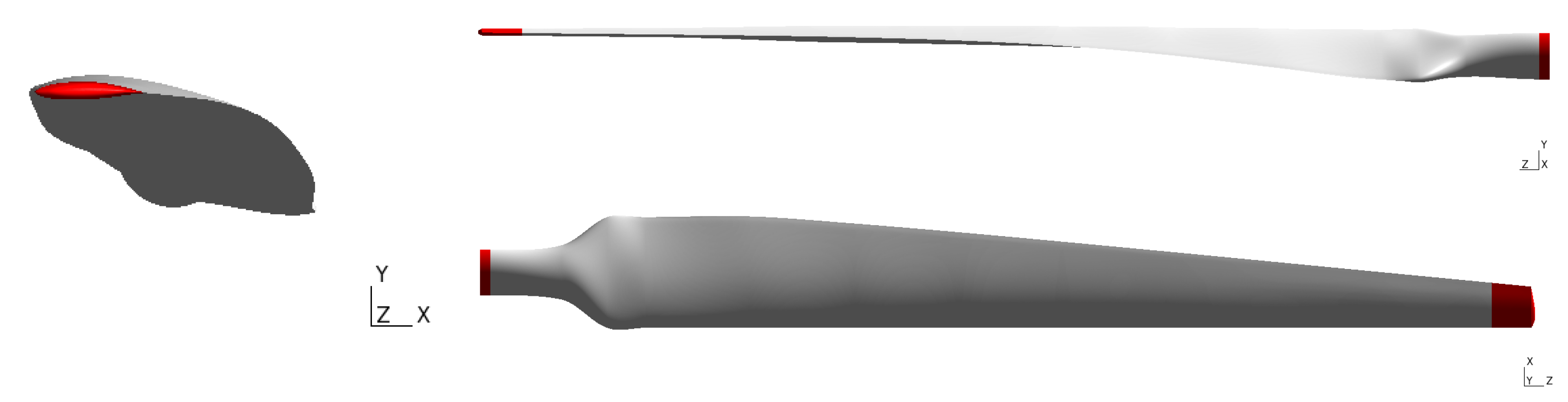
The used coupling meshes are surface meshes of a turbine blade geometry (Wind Turbine Blade created by Ivan Zerpa, 7 February 2012, https://grabcad.com/library/wind-turbine-blade–4) shown in Figure 5. The geometry was triangularized using GMSH [25] fixing the edge-length to achieve an almost uniform element size and shape.
As dummy solvers, we use the Abstract Solver Testing Environment (ASTE) (https://github.com/precice/aste/tree/mapping-tests), a framework, which allows to imitate a parallel solver coupled via preCICE. Each rank reads mesh data from given files and hands it over to preCICE by calling the preCICE Application Programming Interface (API). This allows to inspect various performance characteristics of preCICE without the cost of using a real solver. For data mapping in preCICE, we use the nearest-projection method as introduced in Section 3.
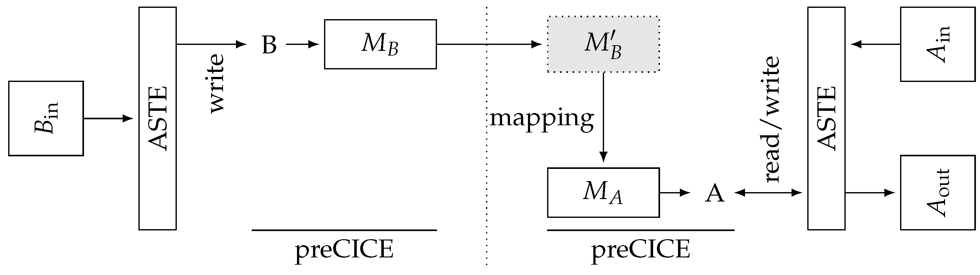
The test case setup involves two ASTE participants B and A. Participant B reads its mesh and provides both the mesh structure and physical data to preCICE. Participant A reads its mesh and provides the mesh structure to preCICE. A then receives both mesh and data from participant B, uses the configured consistent mapping to map the received data to the local mesh and finally writes the resulting vertex data to a file. See Figure 6 for an overview of this process.
4.2. Hardware Description
All measurements are carried out on the SuperMUC-NG supercomputer at the Leibniz Supercomputing Centre of the Bavarian Academy of Science and Humanities (LRZ). This machine consists of 3.1 GHz Intel Xeon Platinum 8174 (SkyLake) processors. Each node contains two processors with 24 cores per processor (48 cores per node) and 96 GB of RAM. The nodes are connected via Intel Omni-Path interconnect.
4.3. Performance Analysis
To show the complexity and scalability improvements in the new preCICE version, we conduct a numerical strong and weak scaling study. For inter-code data exchange, we use TCP/IP sockets communication. In addition, both the overall initialization times and breakdown values are reported in per core average. For all experiments, we avoided synchronization to minimize the cores waiting time and thus the initialization time. This, even though, optimizes the overall initialization time, may slightly reduce the communication-related events breakdown accuracy due to events’ time overlaying.
4.3.1. Strong Scaling
The strong scalability of the developed initialization scheme is evaluated using various computational meshes, which are given in Table 1. To compare the overall performance of the newly developed two-level initialization and the old one-level scheme, we present scalability measurements using mesh M4 (with mesh width 0.005 and 628,898 vertices) as this is the largest mesh that can be handled by both the old and the new version of preCICE. The new two-level initialization scheme would be applicable for much larger meshes as the memory bottleneck induced by sending the complete coupling meshes from A to be via master communication has been eliminated. Accordingly, we also present strong scalability measurements with finer meshes only for the two-level scheme later in this section.
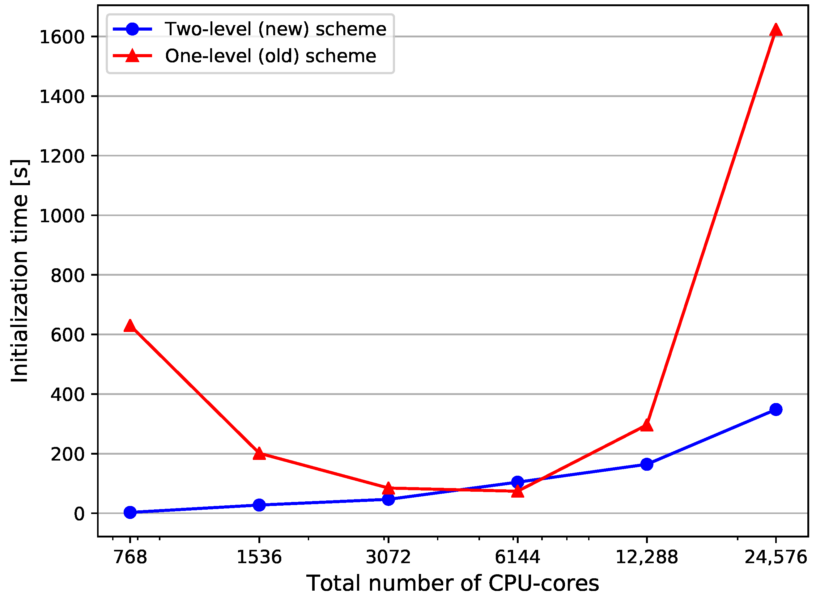
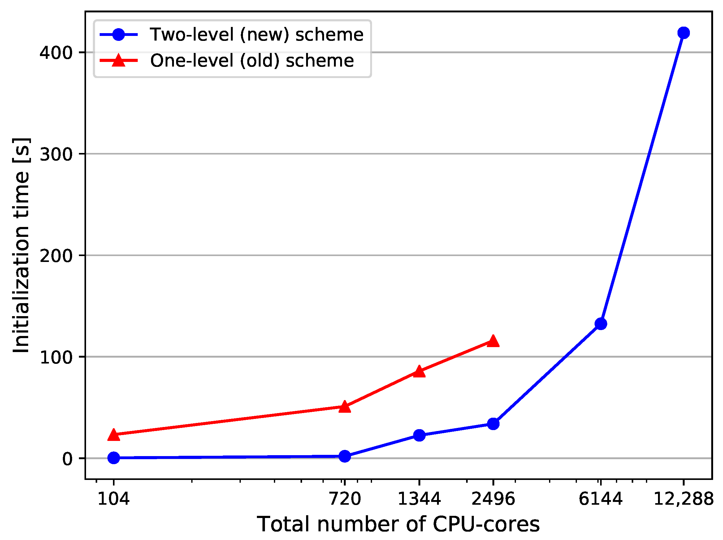
Figure 7 compares the initialization times of both versions using mesh M4. The number of CPU cores indicates the total number of processes, i.e., MPI ranks for both domains together. The available cores are divided between the domains with a ratio 1:3, which ensures, that we do not get matching partitions between both solvers.
The comparison shows, that the new scheme can significantly reduce the initialization time. The improvements are particularly large for large numbers of CPU-cores. The initialization time for 24,576 CPU-cores is less than 6 min for the two-level scheme, while the old scheme requires approximately 5 times more time. All CPU-cores exploited for this experiment are located at the common interface. In a real surface-coupled simulation, the interface ranks are only a small fraction of the total ranks. Therefore, the introduced scheme is expected to be very efficient even when a simulation exploits the whole machine capacity (several hundred thousands of CPU-cores).
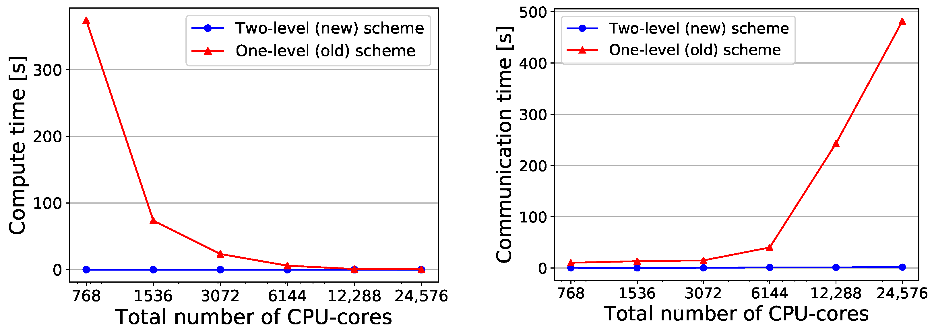
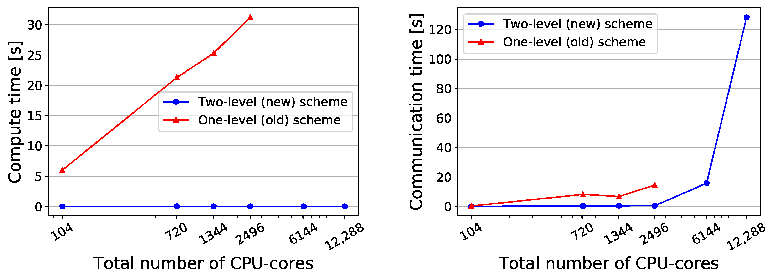
To further analyze the improvement of the preCICE initialization by introducing the new schemes and to explain the runtime evolution for an increasing number of cores, we compare two of the main sub-components of the initialization: Figure 8 compares the mapping computation time (left) and the boundary mesh communication time (right). In the mesh communication phase, coupling solvers exchange their interface mesh partitions (Figure 2, level I). The received mesh partition is filtered and the interpolation is computed in the mapping computation as explained in Section 3 and depicted in Figure 2, level II. Note, that the initialization includes other sub-components, that are not compared, since they are either not executed in both schemes or their contribution is not significant. For instance, the hash-based directory and file naming scheme, explained in Section 2, has significantly reduced the time to establish the communication channels between partner ranks, such that this part of the runtime is now small and not further considered here.
The comparison indicates, that the new scheme has significantly reduced the required time for both. For the mesh communication time, we observe the expected effect of using point-to-point communication in the new scheme instead of master communication in the old scheme: the runtime changes from strongly increasing to almost constant. Figure 8 (left) also clearly showcases the expected strong reduction of runtime in the mapping computation due to the decreasing size of the own mesh partition that each process compares to the partner solver mesh. Figure 8 (right) shows a strong increase of the runtime with increasing number of cores in the one-level scheme for the mesh communication. This can be attributed to partly sequential (in a loop over all processes) feedback collection in the master rank after mesh comparison in all processes and global calculations of vertex interactions between all involved processes in the master process.
In the following, we now focus on further analyzing the runtime and scalability of the new two-level approach in a further breakdown study for both mapping computation (breakdown in Figure 9) and bounding box and mesh communication.
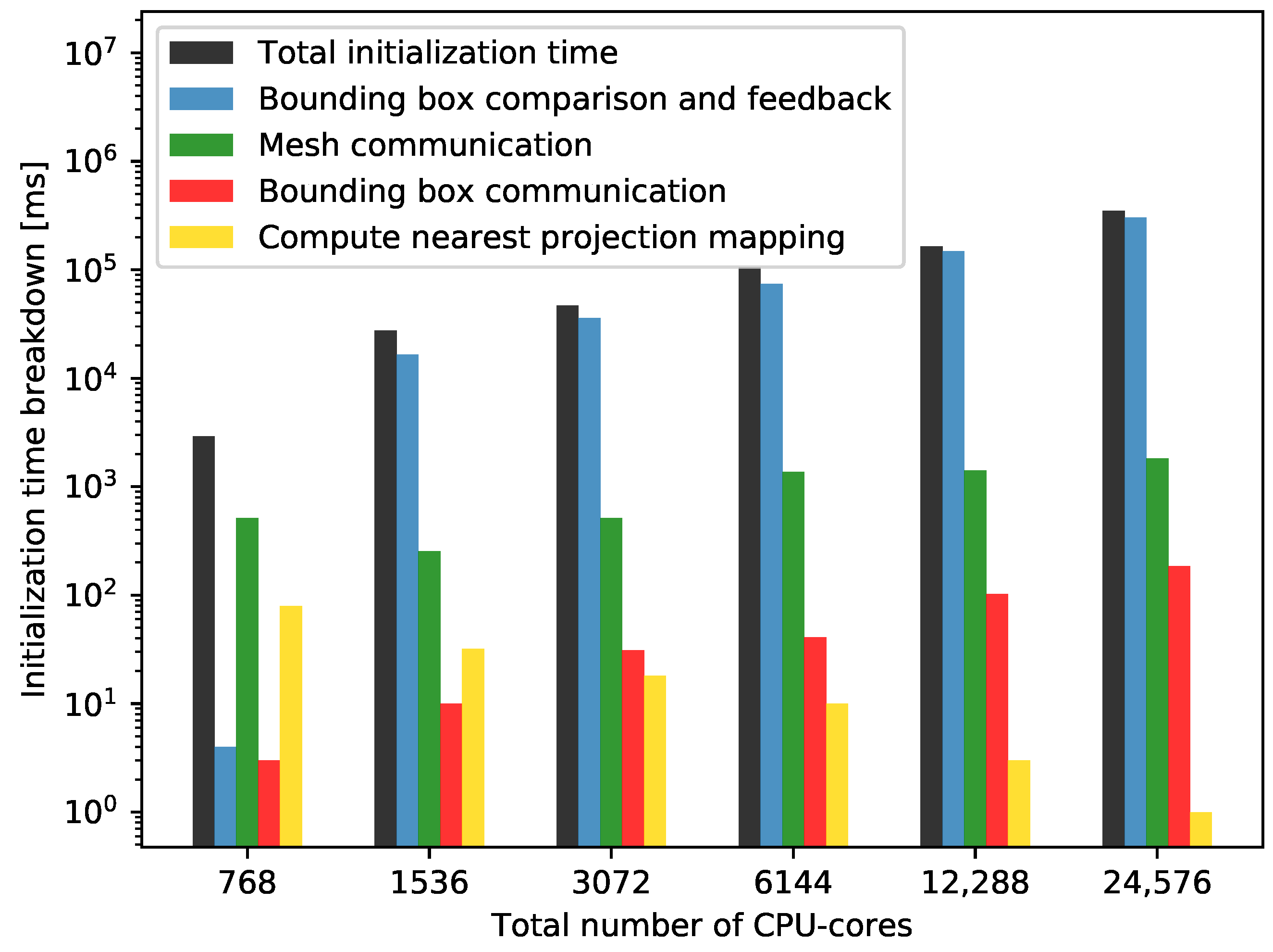
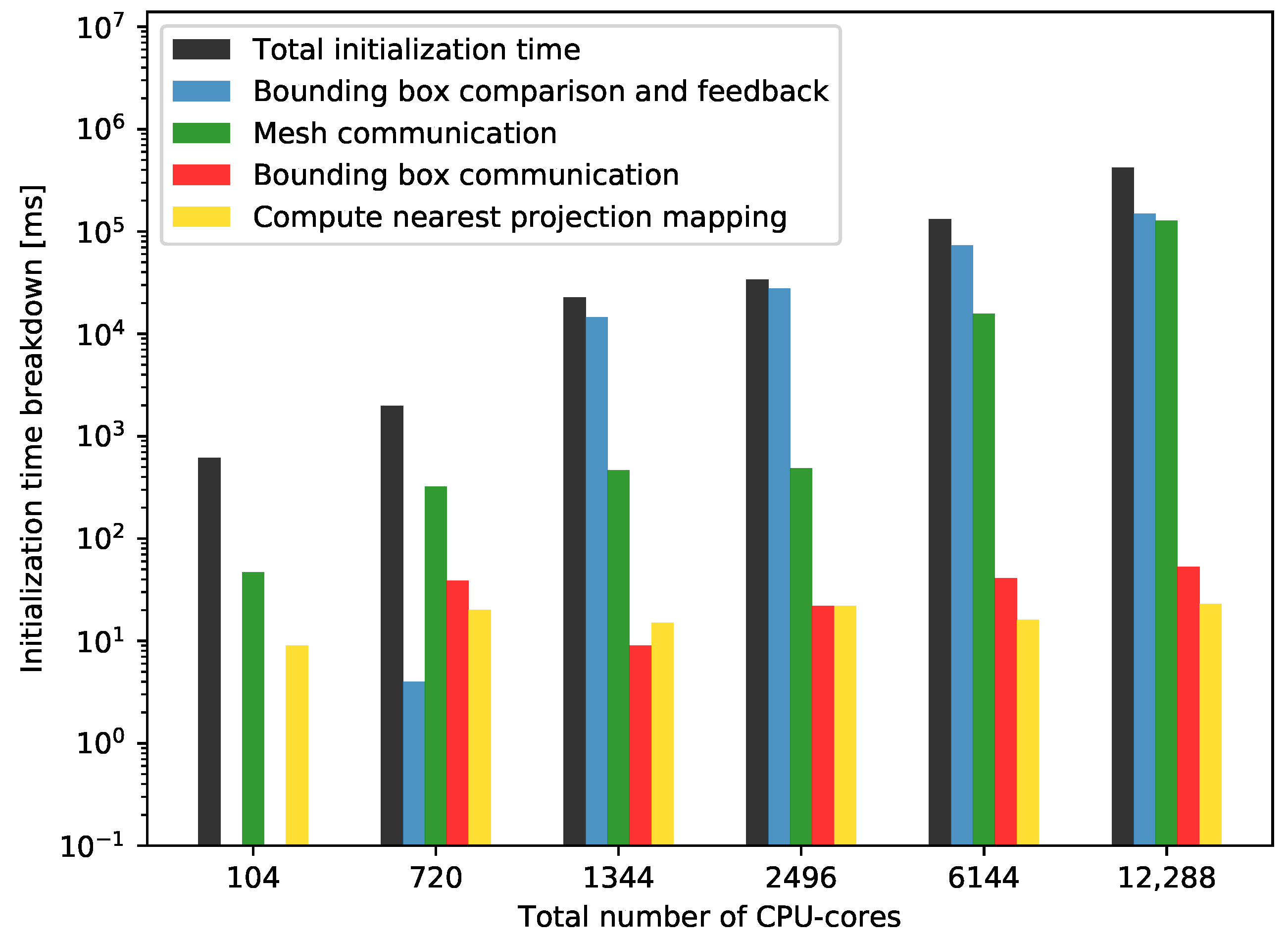
The breakdown of the complete initialization time is given in Figure 10.
The figure shows, that the bounding box comparison and feedback (Figure 1, level II and III) constitute the majority of the runtime for the new two-level initialization, in particular for core counts larger than 1536. The time spent for bounding box comparison increases with the number of processes, which is obvious, as, for a higher number of processes in the partner solver, each process needs to compare its bounding box with more partner processes. Currently, this operation is O() in the number p of processes in total and O(p) per process. In addition, the time spent for feedback, which consists of gathering feedback from processes in the master rank and communicating this to the other solver also increases with the number of processes. This is expected, as the higher number of processes implies an increase in the number of communications in the gather operation.
Figure 10 also shows, that the time required for mesh exchange decreases with increasing number of cores at the beginning and increases for more than 1536 cores. The decrease can be due to the smaller mesh partitions, that are communicated, while the later increase might be because of the higher communication overhead due to an unfavorable distribution of the communication partners on the machine. However, this communication takes only about 1 s and its contribution to the total initialization time is very small.
The time to exchange bounding boxes also increases with increasing number of cores. This is expected, since, for higher core counts, more bounding boxes are gathered in the master rank, communicated via the master ranks and broadcast to the slave ranks of the other solver (Figure 1, levels I to III). This operation is inevitable in the current approach. However, its contribution is very small. Finally, the runtime for the mapping computation decreases with increasing number of cores. This corresponds to our expectations, since a higher number of cores results in smaller mesh partitions, which makes the mesh comparison per pair of mesh partitions cheaper.
A further breakdown of the mapping computation time for nearest projection is shown in Figure 9. Note, that the timings for 12,288 and 24,576 cores are close to the timing resolution and hence difficult to interpret; they were included for completeness. We observe that the indexing, i.e., the neighbor search for triangles as required in the nearest projection mapping, is more expensive than the indexing of edges. This is due to the fact that triangles are more expensive to efficiently index. Furthermore, the lazy indexing strategy prevented the unnecessary indexing of the vertices.
Note, that the current test setup performs a vertex-based partitioning of input meshes, which discards edges and triangles connecting partitions. The amount of triangles and edges discarded grows proportionally to the number of partitions. See Table 2 for a detailed presentation of this effect.
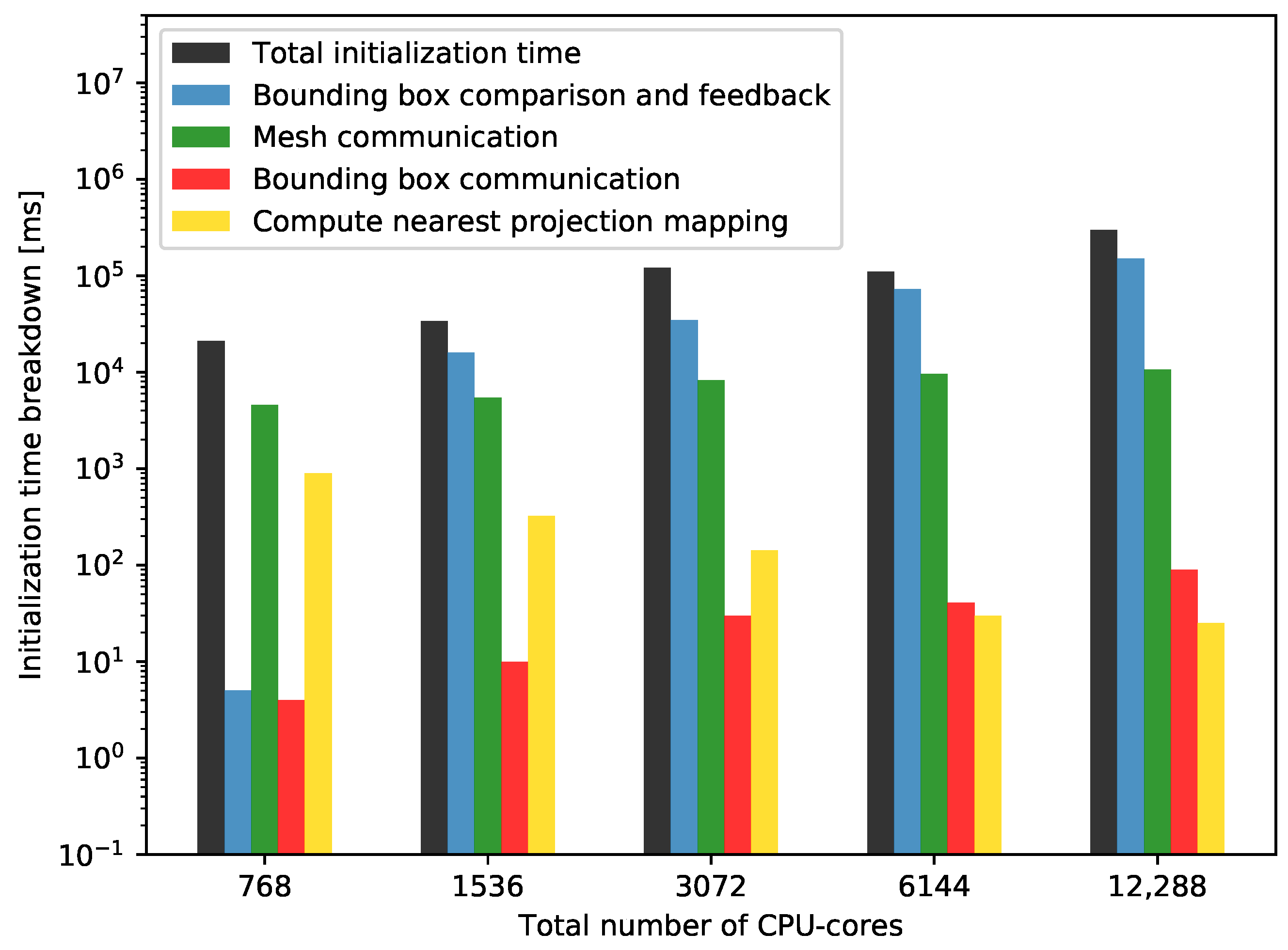
For the further analysis of the performance of the two-level scheme, we present the initialization time breakdown in Figure 11 for the case that coupling solvers use non-matching meshes. For this experiment, we use mesh M5 for solver A and M6 for solver B.
Figure 11 shows, that, even for a finer mesh, the bounding box comparison and feedback are still the most expensive components. The time spent for bounding box communication also increases with increasing number of cores. The cost for these two components is similar to the case with mesh M4 (Figure 10), since the bounding box related cost depends solely on the number of bounding boxes. In addition, we observe a gradual increase in the mesh communication time, which is probably due to a larger communication overhead for the cases with higher core number and, thus, an increasing overall number of messages. The mesh communication time is higher than for the case with mesh M4, which is due to the larger mesh. The most interesting component in this figure is the mapping computation. Even though we use a much finer mesh in this experiment than in Figure 10), the computation time is significantly smaller.
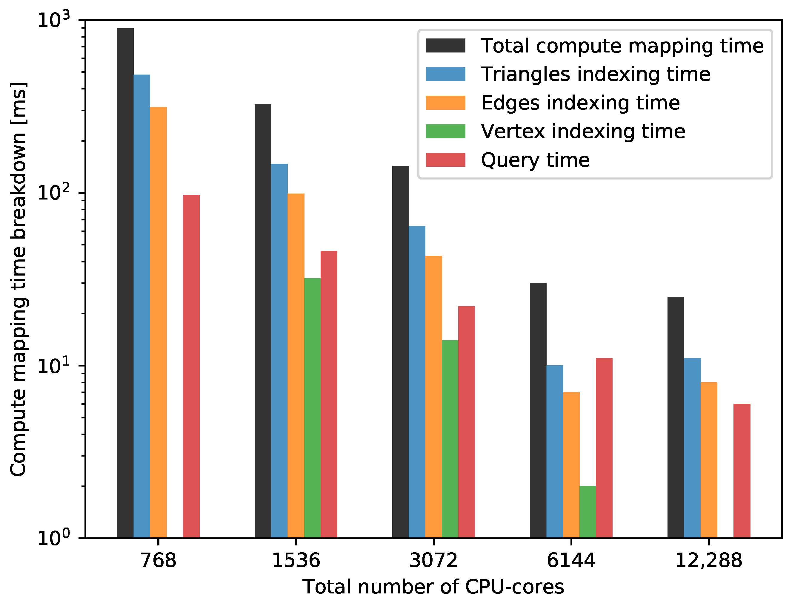
For a detailed analysis of the mapping computation time, we present the breakdown for this case as well in Figure 12. The figure shows the expected scaling for the overall compute time as well as the individual indexing as all parts are of complexity if n is the respective number of mesh entities in each mesh partition. The lazy evaluation is beneficial for the smallest number of cores and, thus, the largest partitions, as it prevents the generation of the vertex index. Higher numbers of cores, in particular 6144 and 12,288, result in partitions, which are small enough for the indexing time to reach the measurement resolution of 1 ms. However, the decreasing query time still indicates the expected behavior due to smaller partitions. Larger meshes and a potentially smaller measurement resolution are required for a conclusive analysis of the upper extreme of the scale.
4.3.2. Weak Scaling
To further analyze the performance of the new initialization scheme, including memory efficiency, we present weak scalability measurements in this section. Table 3 specifies the distribution of compute cores among the solvers A and B for all used meshes. We restrict the measurements for the old initialization scheme to meshes M1–M4, since we run out of memory for larger cases as explained in the last section. Figure 13 compares the initialization time of the new two-level approach and the old scheme for increasing mesh sizes and increasing total number of cores.
A good reduction in initialization time is observed when replacing the old method with the new two-level scheme. Figure 13 shows, that the new scheme significantly reduces the time for the two main components of the initialization stage: the computation of the data mapping and the communication of the interface mesh. In addition, the new scheme is capable of handling very large interface meshes, since it does not use any central mesh communication instance. Even though the initialization time for the finest mesh M6 and 12,288 CPU cores is still in the range of a few minutes, we observe a steep increase for larger meshes, which is due to the increase in mesh communication time as seen in Figure 14 (right).
To analyze the reason of the mentioned performance drop, we present the initialization breakdown for various mesh sizes and CPU cores in Figure 15. We observe, that the mesh communication time increases considerably for meshes M5 and M6. The bounding box communication and comparison cost only depends on the total number of cores, not on the mesh resolution as can be seen in a comparison of Figure 10 and Figure 15. For the mapping computation, we observe an almost constant runtime, which is expected as a result of the constant mesh partition size per core. The improvement of the two most costly parts—bounding box comparison and mesh communication—is work in progress. For bounding box communication, this has already been sketched in Section 4.3.1. For mesh communication, further analysis of potential bottlenecks such as synchronization issues is required.
5. Conclusions
We tackled two bottlenecks of the initialization of the coupling library preCICE. Firstly, we replaced the previous gather-scatter mesh comparison by a parallel two-level scheme. Secondly, we improved the mesh filtering of the nearest-projection data mapping from previously to now .
To evaluate the proposed algorithms, we presented strong and weak scaling measurements for an artificial turbine blade test case using various mesh resolutions. The performance analysis showed, that we can achieve five times faster initialization with the new implementations on 24,576 (interface) cores using a coupling interface mesh with 628,898 vertices. By avoiding the memory bottleneck of the old one-level (gather-scatter) scheme, we were in addition able to handle much larger meshes. The largest surface mesh we considered had nearly three million vertices, which, in a real simulation, could correspond to a coupled setup running on a complete supercomputer (several hundred thousands of cores). We were able to initialize this setup in less than six minutes.
Our analysis revealed, that the most expensive component of the new scheme is the comparison of bounding boxes and the sending of connection feedback to the coupling partner. Using more efficient data structures such as linked-cells to store the set of bounding boxes could potentially further improve the initialization.
Author Contributions
Conceptualization, A.T., F.S., B.U. and M.S.; software, A.T., F.S. and B.U.; validation, A.T. and F.S.; writing—original draft preparation, A.T., F.S. and B.U.; writing—review and editing, B.U. and M.S.; visualization, A.T. and F.S.; supervision, B.U. and M.S.; project administration, M.S.; funding acquisition, M.S. All authors have read and agreed to the published version of the manuscript.
Funding
This work was funded by Deutsche Forschungsgemeinschaft (DFG, German Research Foundation) under Germany’s Excellence Strategy—EXC 2075—390740016, through the project preDOM 391150578, International Graduate Research Group on “Soft Tissue Robotics” (GRK 2198/1) and the Priority Program 1648—SPPEXA; the European Union’s Horizon 2020 research and innovation program under the Marie Sklodowska-Curie grant agreement No. 754462; and the Competence Network for Scientific High Performance Computing in Bavaria (KONWIHR).
Institutional Review Board Statement
Not applicable.
Informed Consent Statement
Not applicable.
Data Availability Statement
The data presented in this study are openly available. Please refer to the paper text for the resource repositories.
Acknowledgments
We acknowledge the support by the Stuttgart Center for Simulation Science (SimTech). The performance measurements were carried out on SuperMUC-NG at Leibniz Rechenzentrum (LRZ).
Conflicts of Interest
The authors declare no conflict of interest.
References
- Cinquegrana, D.; Vitagliano, P.L. Validation of a new fluid—Structure interaction framework for non-linear instabilities of 3D aerodynamic configurations. J. Fluids Struct. 2021, 103, 103264. [Google Scholar] [CrossRef]
- Naseri, A.; Totounferoush, A.; González, I.; Mehl, M.; Pérez-Segarra, C.D. A scalable framework for the partitioned solution of fluid–structure interaction problems. Comput. Mech. 2020, 66, 471–489. [Google Scholar] [CrossRef]
- Totounferoush, A.; Naseri, A.; Chiva, J.; Oliva, A.; Mehl, M. A GPU Accelerated Framework for Partitioned Solution of Fluid-Structure Interaction Problems. In Proceedings of the 14th WCCM-ECCOMAS Congress 2020, online, 11–15 January 2021; Volume 700. [Google Scholar]
- Jaust, A.; Weishaupt, K.; Mehl, M.; Flemisch, B. Partitioned coupling schemes for free-flow and porous-media applications with sharp interfaces. In Finite Volumes for Complex Applications IX—Methods, Theoretical Aspects, Examples; Klöfkorn, R., Keilegavlen, E., Radu, F.A., Fuhrmann, J., Eds.; Springer International Publishing: Cham, Switzerland, 2020; pp. 605–613. [Google Scholar] [CrossRef]
- Revell, A.; Afgan, I.; Ali, A.; Santasmasas, M.; Craft, T.; de Rosis, A.; Holgate, J.; Laurence, D.; Iyamabo, B.; Mole, A.; et al. Coupled hybrid RANS-LES research at the university of manchester. ERCOFTAC Bull. 2020, 120, 67. [Google Scholar]
- Bungartz, H.J.; Lindner, F.; Mehl, M.; Scheufele, K.; Shukaev, A.; Uekermann, B. Partitioned fluid-structure-acoustics interaction on distributed data—Coupling via preCICE. In Software for Exascale Computing—SPPEXA 2013–2015; Bungartz, H.J., Neumann, P., Nagel, E.W., Eds.; Springer: Cham, Switzerland, 2016. [Google Scholar] [CrossRef]
- Lindner, F.; Mehl, M.; Uekermann, B. Radial basis function interpolation for black-box multi-physics simulations. In Proceedings of the VII International Conference on Coupled Problems in Science and Engineering (CIMNE), Rhodes Island, Greece, 12–14 June 2017; pp. 50–61. [Google Scholar]
- Mehl, M.; Uekermann, B.; Bijl, H.; Blom, D.; Gatzhammer, B.; Zuijlen, A. Parallel coupling numerics for partitioned fluid-structure interaction simulations. Comput. Math. Appl. 2016, 71, 869–891. [Google Scholar] [CrossRef]
- Scheufele, K.; Mehl, M. Robust multisecant Quasi-Newton variants for parallel Fluid-Structure simulations—And other multiphysics applications. SIAM J. Sci. Comput. 2017, 39, S404–S433. [Google Scholar] [CrossRef]
- Haelterman, R.; Bogaers, A.; Uekermann, B.; Scheufele, K.; Mehl, M. Improving the performance of the partitioned QN-ILS procedure for fluid-structure interaction problems: Filtering. Comput. Struct. 2016, 171, 9–17. [Google Scholar] [CrossRef]
- Uekermann, B. Partitioned Fluid-Structure Interaction on Massively Parallel Systems. Ph.D. Thesis, Department of Informatics, Technical University of Munich, Munich, Germany, 2016. [Google Scholar] [CrossRef]
- Lindner, F. Data Transfer in Partitioned Multi-Physics Simulations: Interpolation and Communication. Ph.D. Thesis, University of Stuttgart, Stuttgart, Germany, 2019. [Google Scholar] [CrossRef]
- Lindner, F.; Totounferoush, A.; Mehl, M.; Uekermann, B.; Pour, N.E.; Krupp, V.; Roller, S.; Reimann, T.; Sternel, D.C.; Egawa, R.; et al. ExaFSA: Parallel Fluid-Structure-Acoustic Simulation. In Software for Exascale Computing—SPPEXA 2016–2019; Springer: Cham, Switzerland, 2020; pp. 271–300. [Google Scholar] [CrossRef]
- Wolf, K.; Bayrasy, P.; Brodbeck, C.; Kalmykov, I.; Oeckerath, A.; Wirth, N. MpCCI: Neutral interfaces for multiphysics simulations. In Scientific Computing and Algorithms in Industrial Simulations; Springer: Cham, Switzerland, 2017; pp. 135–151. [Google Scholar] [CrossRef]
- Joppich, W.; Kürschner, M. MpCCI—A tool for the simulation of coupled applications. Concurr. Comput. Pract. Exp. 2006, 18, 183–192. [Google Scholar] [CrossRef]
- Slattery, S.; Wilson, P.; Pawlowski, R. The data transfer kit: A geometric rendezvous-based tool for multiphysics data transfer. In Proceedings of the International Conference on Mathematics & Computational Methods Applied to Nuclear Science & Engineering (M&C 2013), Sun Valley, ID, USA, 5–9 May 2013; pp. 5–9. [Google Scholar]
- Plimpton, S.J.; Hendrickson, B.; Stewart, J.R. A parallel rendezvous algorithm for interpolation between multiple grids. J. Parallel Distrib. Comput. 2004, 64, 266–276. [Google Scholar] [CrossRef]
- Duchaine, F.; Jauré, S.; Poitou, D.; Quémerais, E.; Staffelbach, G.; Morel, T.; Gicquel, L. Analysis of high performance conjugate heat transfer with the openpalm coupler. Comput. Sci. Discov. 2015, 8, 015003. [Google Scholar] [CrossRef] [Green Version]
- Tang, Y.H.; Kudo, S.; Bian, X.; Li, Z.; Karniadakis, G.E. Multiscale universal interface: A concurrent framework for coupling heterogeneous solvers. J. Comput. Phys. 2015, 297, 13–31. [Google Scholar] [CrossRef] [Green Version]
- Thomas, D.; Cerquaglia, M.L.; Boman, R.; Economon, T.D.; Alonso, J.J.; Dimitriadis, G.; Terrapon, V.E. CUPyDO-An integrated Python environment for coupled fluid-structure simulations. Adv. Eng. Softw. 2019, 128, 69–85. [Google Scholar] [CrossRef]
- De Boer, A.; van Zuijlen, A.; Bijl, H. Comparison of conservative and consistent approaches for the coupling of non-matching meshes. Comput. Methods Appl. Mech. Eng. 2008, 197, 4284–4297. [Google Scholar] [CrossRef]
- Boost. Boost Library. Available online: http://www.boost.org/ (accessed on 15 April 2021).
- Beckmann, N.; Kriegel, H.P.; Schneider, R.; Seeger, B. The R*-tree: An efficient and robust access method for points and rectangles. In Proceedings of the 1990 ACM SIGMOD International Conference on Management of Data, Atlantic City, NJ, USA, 23–25 May 1990; pp. 322–331. [Google Scholar] [CrossRef] [Green Version]
- Guttman, A. R-trees: A dynamic index structure for spatial searching. In Proceedings of the 1984 ACM SIGMOD International Conference on Management of Data, Boston, MA, USA, 18–21 June 1984; pp. 47–57. [Google Scholar] [CrossRef]
- Geuzaine, C.; Remacle, J.F. Gmsh: A 3-D finite element mesh generator with built-in pre-and post-processing facilities. Int. J. Numer. Methods Eng. 2009, 79, 1309–1331. [Google Scholar] [CrossRef]
Figure 1.
Two-level initialization scheme: the first level exchanges bounding boxes and establishes the communication channels between partner processes. The master processes of B gathers the bounding boxes from other processes (I) and sends them to the master process of solver A (II). The master process of solver A broadcasts the received bounding boxes to all other processes of solver A (III). Each process of A compares the received set of bounding boxes to its own bounding box to find the partner processes in solver B (IV). The complete set of sent bounding boxes is drawn in black, while the green boxes represent the subset relevant for the respective process of solver A. The filtered set of bounding boxes is communicated to the processes of solver B via master communication, such that not only the processes of solver A, but also the processes of solver B know their potential communication partners (V).

Figure 2.
Two-level initialization scheme: the second level exchanges mesh partitions between partner processes to identify the exact list of data that have to be communicated during the simulation. Each process of solver B directly communicates its mesh partition to the relevant partner processes of solver A (I), that have been identified in level one. Each process of solver A compares its own mesh partition to the received mesh partitions and identifies, which data must be communicated during run time (II). The complete received mesh partitions are drawn in black while, the parts that actually have to be communicated in green.

Figure 3.
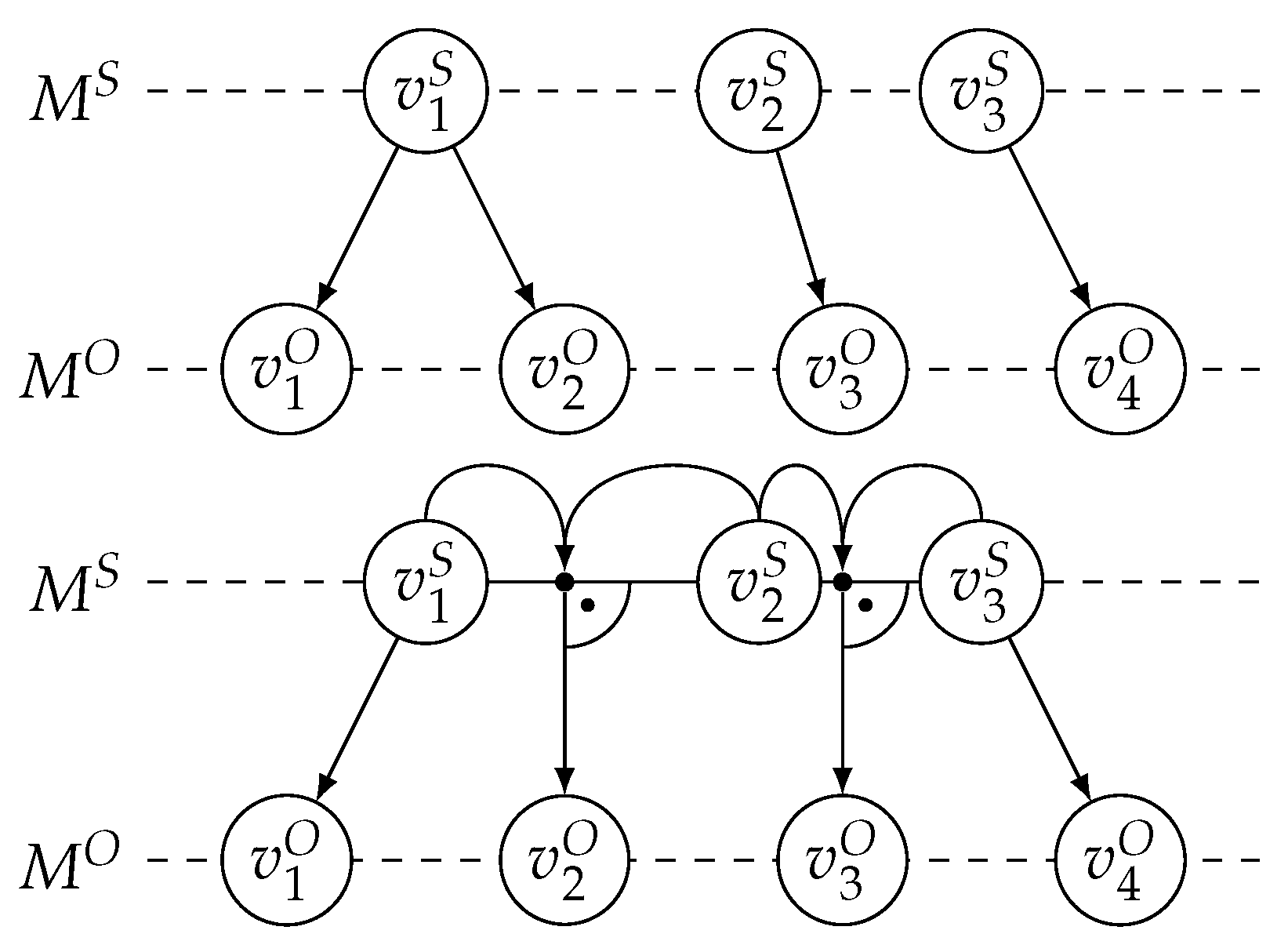
Comparison of the nearest-neighbour mapping (top) and the nearest-projection mapping (bottom). Both mappings are consistent and map from the search mesh to the origin mesh . The nearest-projection mapping prevents extrapolation by mapping to the closest vertex for and . The vertices and are projected onto the edges and , resulting in interpolation.
Figure 3.
Comparison of the nearest-neighbour mapping (top) and the nearest-projection mapping (bottom). Both mappings are consistent and map from the search mesh to the origin mesh . The nearest-projection mapping prevents extrapolation by mapping to the closest vertex for and . The vertices and are projected onto the edges and , resulting in interpolation.

Figure 4.
Spatial lookup for nearest-projection mapping: The selection zones of the cascading algorithm used by the nearest-projection onto a single triangle ABC. If the location of the orthogonal projection of the original data point is outside of ABC, the projection onto edges are considered before finally projecting onto vertices. The image on the right describes the order in which the zones are considered.

Figure 5.
Different perspectives on the turbine-blade test geometry.

Figure 6.
Test configuration using ASTE. Participant B on the left reads the mesh structure and physical data from a file . Participant A on the right reads the mesh structure from the file . B and A initialize communication, then data are transferred from to , mapped to using a nearest-projection mapping and finally written to a file .

Figure 7.
Strong scalability measurements: Total initialization time comparison between the two-level approach and the previously used one-level scheme. A mesh with mesh width 0.005 and 628,898 vertices (Table 1, M4) is used for conducting the analysis.
Figure 7.
Strong scalability measurements: Total initialization time comparison between the two-level approach and the previously used one-level scheme. A mesh with mesh width 0.005 and 628,898 vertices (Table 1, M4) is used for conducting the analysis.

Figure 8.
Strong scalability measurements: Comparison of run times for mapping computation (left) and mesh communication (right) between between the two-level and the one-level scheme. The mesh M4 is used for conducting the analysis.
Figure 8.
Strong scalability measurements: Comparison of run times for mapping computation (left) and mesh communication (right) between between the two-level and the one-level scheme. The mesh M4 is used for conducting the analysis.

Figure 9.
Strong scalability measurements: Breakdown of the mapping computation time of the two-level approach. The mesh M4 is used for conducting the analysis.
Figure 9.
Strong scalability measurements: Breakdown of the mapping computation time of the two-level approach. The mesh M4 is used for conducting the analysis.

Figure 10.
Strong scalability measurements: Initialization time breakdown for the two-level initialization approach using mesh M4. Only parts significantly contributing to the runtime are depicted: 1—Bounding box comparison and feedback (Figure 1 levels IV and V). 2—Mesh communication (Figure 2 levels II). 3—Bounding box communication (Figure 1 levels II and III). 4—Compute nearest projection mapping (Figure 2 level II).

Figure 11.
Strong scalability measurements: Initialization time breakdown for the two-level initialization approach using mesh M5 for solver A and mesh M6 for B. Only parts significantly contributing to the runtime are depicted: 1—Bounding box comparison and feedback (Figure 1 levels IV and V). 2—Mesh communication (Figure 2 levels II). 3—Bounding box communication (Figure 1 levels II and III). 4—Compute nearest projection mapping (Figure 2 level II).

Figure 12.
Strong scalability measurements: Breakdown of the mapping computation time of the two-level approach. The mapping projects vertices from mesh M5 onto connectivity information of mesh M6.
Figure 12.
Strong scalability measurements: Breakdown of the mapping computation time of the two-level approach. The mapping projects vertices from mesh M5 onto connectivity information of mesh M6.

Figure 13.
Weak scalability measurements: Total initialization time comparison between the two-level and the one-level schemes. The core distribution and the mesh information are given in Table 3.
Figure 13.
Weak scalability measurements: Total initialization time comparison between the two-level and the one-level schemes. The core distribution and the mesh information are given in Table 3.

Figure 14.
Weak scalability measurements: Comparison of mapping computation (left) and mesh communication (right) time between the two-level and the one-level scheme. The core distribution and the mesh information are given in Table 3.
Figure 14.
Weak scalability measurements: Comparison of mapping computation (left) and mesh communication (right) time between the two-level and the one-level scheme. The core distribution and the mesh information are given in Table 3.

Figure 15.
Weak scalability measurements: Initialization time breakdown for the two-level initialization scheme. Only algorithmic parts with significant contributions to the initialization runtime are depicted: 1—Bounding box comparison and feedback (Figure 1 levels IV and V). 2—Mesh communication (Figure 2 levels II). 3—Bounding box communication (Figure 1 levels II and III). 4—Compute nearest projection mapping (Figure 2 level II). The core distribution and the mesh information are given in Table 3.


Table 1.
Strong scalability measurements: Meshes for the wind turbine blade at varying mesh resolutions (mesh width). The mesh width indicates the average edge length used to construct the surface mesh.
Table 1.
Strong scalability measurements: Meshes for the wind turbine blade at varying mesh resolutions (mesh width). The mesh width indicates the average edge length used to construct the surface mesh.
| Mesh ID | Mesh Width | Number of Vertices | Number of Triangles |
|---|---|---|---|
| M4 | 0.0005 | 628,898 | 1,257,391 |
| M5 | 0.0004 | 1,660,616 | 3,321,140 |
| M6 | 0.0003 | 2,962,176 | 5,924,260 |
Table 2.
Number of triangles of mesh 4 and mesh M6 that are discarded due to the vertex-based partitioning (in absolute and relative values). The original mesh M4 contains 1,257,391 triangles and the original M6 mesh contains 5,924,260 triangles.
Table 2.
Number of triangles of mesh 4 and mesh M6 that are discarded due to the vertex-based partitioning (in absolute and relative values). The original mesh M4 contains 1,257,391 triangles and the original M6 mesh contains 5,924,260 triangles.
| Cores | M4 | M6 | ||||
|---|---|---|---|---|---|---|
| Total | B | A | Lost Triangles | Rel [%] | Lost Triangles | Rel [%] |
| 768 | 192 | 576 | 44,244 | 3.52 | 90,195 | 1.52 |
| 1536 | 384 | 1152 | 62,003 | 4.93 | 154,358 | 2.61 |
| 3072 | 768 | 2304 | 86,085 | 6.85 | 246,937 | 4.17 |
| 6144 | 1536 | 4608 | 118,313 | 9.41 | 376,108 | 6.35 |
| 12,288 | 3072 | 9216 | 165,085 | 13.13 | 552,797 | 9.33 |
| 24,576 | 6144 | 18,432 | 230,556 | 18.34 | 797,042 | 13.45 |
Table 3.
Weak scalability measurements: Meshes for the wind turbine blade at varying mesh resolution (mesh width). The mesh width indicates the average edge length used to construct the surface mesh. The total number of cores is approximately proportional to the number of mesh vertices. The available CPU cores are distributed with a 1:3 ratio between the solvers.
| Mesh | Mesh | #Vertices | Cores | #Vertices per Core | |||
|---|---|---|---|---|---|---|---|
| ID | Width | Total | Total | B | A | B | A |
| M1 | 0.0025 | 25,722 | 104 | 26 | 78 | 989 | 330 |
| M2 | 0.0010 | 165,009 | 720 | 192 | 528 | 859 | 312 |
| M3 | 0.00075 | 330,139 | 1344 | 336 | 1008 | 982 | 328 |
| M4 | 0.0005 | 628,898 | 2496 | 624 | 1872 | 1007 | 336 |
| M5 | 0.0004 | 1,660,616 | 6144 | 1536 | 4608 | 1081 | 361 |
| M6 | 0.0003 | 2,962,176 | 12,288 | 3072 | 9216 | 964 | 321 |
Publisher’s Note: MDPI stays neutral with regard to jurisdictional claims in published maps and institutional affiliations. |
© 2021 by the authors. Licensee MDPI, Basel, Switzerland. This article is an open access article distributed under the terms and conditions of the Creative Commons Attribution (CC BY) license (https://creativecommons.org/licenses/by/4.0/).
Share and Cite
MDPI and ACS Style
Totounferoush, A.; Simonis, F.; Uekermann, B.; Schulte, M. Efficient and Scalable Initialization of Partitioned Coupled Simulations with preCICE. Algorithms 2021, 14, 166. https://0-doi-org.brum.beds.ac.uk/10.3390/a14060166
AMA Style
Totounferoush A, Simonis F, Uekermann B, Schulte M. Efficient and Scalable Initialization of Partitioned Coupled Simulations with preCICE. Algorithms. 2021; 14(6):166. https://0-doi-org.brum.beds.ac.uk/10.3390/a14060166
Chicago/Turabian StyleTotounferoush, Amin, Frédéric Simonis, Benjamin Uekermann, and Miriam Schulte. 2021. "Efficient and Scalable Initialization of Partitioned Coupled Simulations with preCICE" Algorithms 14, no. 6: 166. https://0-doi-org.brum.beds.ac.uk/10.3390/a14060166
Note that from the first issue of 2016, this journal uses article numbers instead of page numbers. See further details here.