Damage Identification of Long-Span Bridges Using the Hybrid of Convolutional Neural Network and Long Short-Term Memory Network

Abstract

The shallow features extracted by the traditional artificial intelligence algorithm-based damage identification methods pose low sensitivity and ignore the timing characteristics of vibration signals. Thus, this study uses the high-dimensional feature extraction advantages of convolutional neural networks (CNNs) and the time series modeling capability of long short-term memory networks (LSTM) to identify damage to long-span bridges. Firstly, the features extracted by CNN and LSTM are fused as the input of the fully connected layer to train the CNN-LSTM model. After that, the trained CNN-LSTM model is employed for damage identification. Finally, a numerical example of a large-span suspension bridge was carried out to investigate the effectiveness of the proposed method. Furthermore, the performance of CNN-LSTM and CNN under different noise levels was compared to test the feasibility of application in practical engineering. The results demonstrate the following: (1) the combination of CNN and LSTM is satisfactory with 94% of the damage localization accuracy and only 8.0% of the average relative identification error (ARIE) of damage severity identification; (2) in comparison to the CNN, the CNN-LSTM results in superior identification accuracy; the damage localization accuracy is improved by 8.13%, while the decrement of ARIE of damage severity identification is 5.20%; and (3) the proposed method is capable of resisting the influence of environmental noise and acquires an acceptable recognition effect for multi-location damage; in a database with a lower signal-to-noise ratio of 3.33, the damage localization accuracy of the CNN-LSTM model is 67.06%, and the ARIE of the damage severity identification is 31%. This work provides an innovative idea for damage identification of long-span bridges and is conducive to promote follow-up studies regarding structural condition evaluation.

1. Introduction

Owing to the joint effect of the tough service environment and the long-term over-limit load, bridges will inevitably suffer deterioration during operation. Thus, health monitoring systems have been widely used in the condition alarming of long-span bridges. Accordingly, the comprehensive exploitation of bridge monitoring information and accurate identification of the location and extent of damage is of crucial scientific research significance and engineering application value to ensure bridge safety and smooth road networks [1].

The essence of structural damage identification is the problem of pattern recognition, which can be realized using artificial intelligence algorithms [2,3]. Generally, traditional artificial intelligence algorithm-based damage identification methods include two steps: (i) extraction of damage sensitive features (DSFs). Time series analysis, frequency spectrum analysis, statistical analysis, and other means are used to extract features that characterize the damage state from the structural response [4,5]; (ii) prediction of damage. Artificial intelligence algorithms are employed to establish the mapping relationship between DSFs and damage location and severity [6,7]. For instance, Arangio et al. [8] utilized probabilistic logic methods to develop a two-step Bayesian framework for damage localization and extent prediction of the suspension bridge main cables and hangers. Casciati et al. [9] applied the firefly and the artificial bee colony algorithms to diagnose the damage caused by the decrease in stiffness of the cable and main beam. Due to the high uncertainty of the measurement and finite element modeling, Ding et al. [10] established the objective function using modal data and sparse regularization technology, and they developed a hybrid group intelligence technology involving the Jaya and tree-seed algorithm to identify structural damage. Meng et al. [11] used modal flexibility as DSF and performed damage diagnosis of suspension bridge hangers based on a genetic algorithm. Guan et al. [12] recruited wavelet coefficient modulus maxima as DSF and employed an artificial neural network (ANN) and particle swarm algorithm to complete the damage identification of a suspension bridge. Seyedpoor et al. [13] developed a two-step structural damage identification method. First, the support vector machine was used to initially determine the damage location to reduce the search space dimension, and then, the evolutionary algorithm was used to accurately and quickly search for the damage location. The above study shows that current research on conventional artificial intelligence algorithms-based damage identification methods mainly focuses on traditional machine learning and evolutionary algorithms. However, traditional machine learning algorithms, such as ANN and naive Bayes, are shallow learning. The trained model has insufficient ability to recognize complicated nonlinear damage, and the accuracy largely depends on the sensitivity of the selected DSFs. Meanwhile, it is easy to fall into the local optimal solution problem during the solution process of evolutionary algorithms. Hence, it is essential to explore more effective ways to solve the aforementioned issues.

In 2006, Hinton et al. [14] proposed deep belief networks and introduced a layer-by-layer pre-training method, which laid the foundation for the development of deep learning. Shallow learning mostly relies on manual experience or feature conversion methods to obtain features. In contrast, deep learning processes the original data through multilayer nonlinear transformation, and then, it outputs higher-dimensional and more abstract features, thereby avoiding complicated and repetitive feature engineering.

Convolutional neural networks (CNNs) and long short-term memory networks (LSTM), which are of great application value, have gradually captured widespread attention from scholars in the engineering field. Various research studies have been conducted, which can be summarized into three aspects. (i) Structural defects detecting. Cha et al. [15] designed a concrete crack detection method combining computer vision (CV) and CNN, which can detect concrete cracks, steel corrosion, bolt corrosion, and steel delamination. Gao et al. [16] introduced VGGNet for structural damage detection through transfer learning technology, which shows that transfer learning technology has broad application prospects in image-based structural defects recognition. Xu et al. [17] formulated a framework for crack recognition and extraction of bridge steel box girders based on a restricted Boltzmann machine. (ii) Structural damage identification. Lin et al. [18] devised a CNN-based damage recognition method to accurately identify the damage location and degree of the simply supported beam finite element model and automatically learn the low order of the mode shape. Abdeljaber et al. [19] used the vibration response signal as the model input for the CNN and separately trained the model for each node of the planar steel frame structure to determine the bolt connection state. Yu et al. [20] proposed a novel method based on deep CNNs for identifying and locating damage to building structures equipped with intelligent control equipment. (iii) Data processing and state prediction. Bao et al. [21] work out an anomaly detection method of structural health monitoring data based on CV and CNN. Zhang et al. [22] applied the advantages of LSTM to model time series changes and used it to predict the depth of groundwater levels in agricultural areas. Zhang et al. [23] utilized LSTM for sewer overflow monitoring and achieved better results than multilayer perception and wavelet neural networks. The above-mentioned research demonstrates that CNN does have a superior performance in feature extraction, and LSTM also has unique advantages in describing time series changes.

Recently, the hybrid architecture of CNN and LSTM has been widely adopted due to its outstanding performance. For instance, Yang et al. [24] introduced CNN-LSTM architecture to non-contact computer vision-based vibration measurement and used the structural vibration video to identify its basic modal frequency. Zhao et al. [25] employed the hybrid architecture to establish the mapping relationship between the external excitation and the nonlinear response, thereby detecting the early damage of the structure. Petmezas et al. [26] proposed to use the CNN-LSTM model to help clinicians detect common atrial fibrillation in real time on routine screening electrocardiograms. Wigington et al. [27] utilized the CNN-LSTM model for handwritten font recognition, which significantly reduced the word error rate and character error rate. Qiao et al. [28] proposed a short-term traffic flow prediction method based on the 1DCNN-LSTM model, which aims to effectively solve traffic travel and management problems. Evidently, the CNN-LSTM architecture can fully combine the advantages of these two independent models, which is demonstrated to fulfill more complicated tasks.

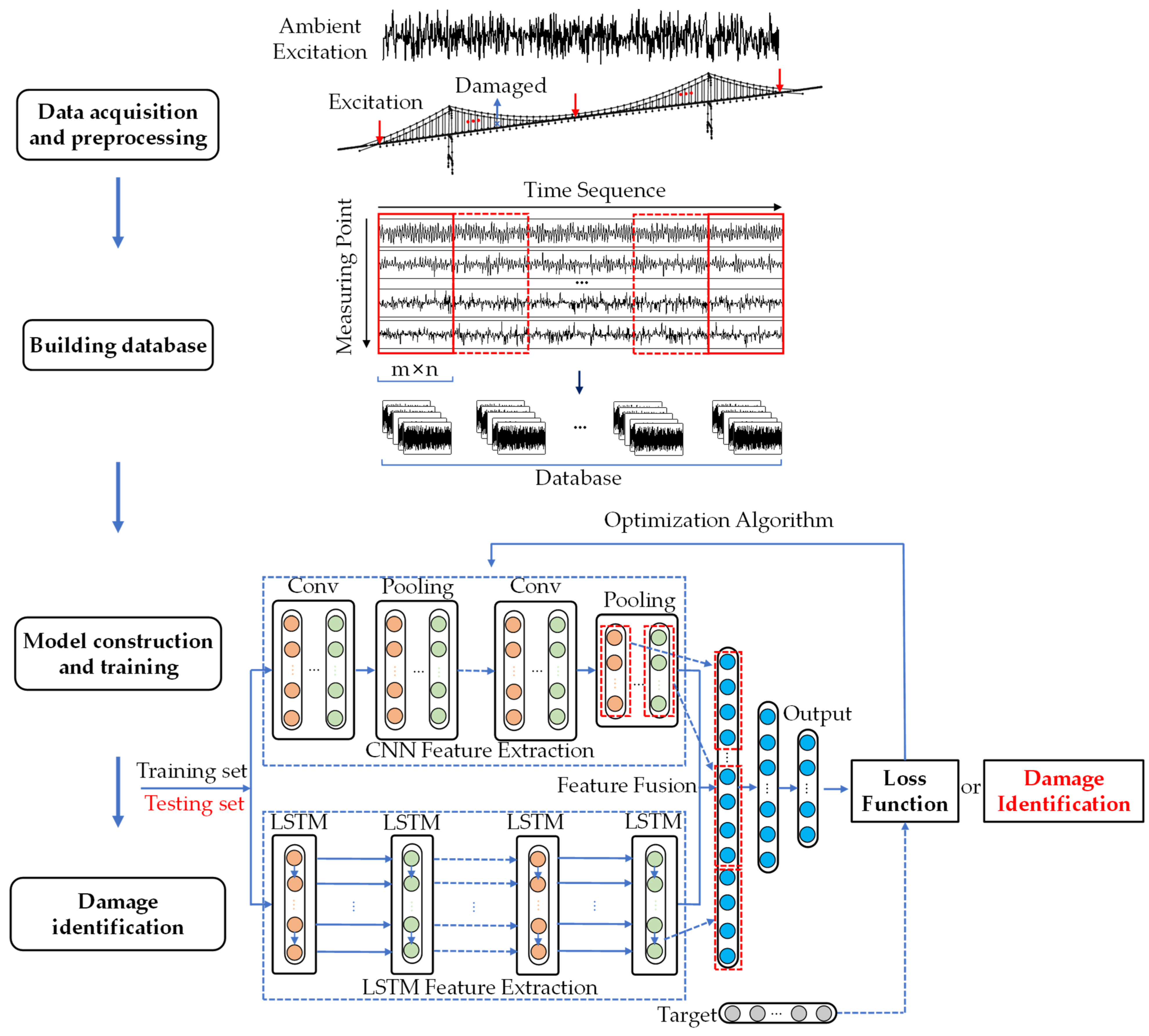
From the above literature review, the following conclusions can be drawn: (1) Shallow features used for damage identification are usually not suitable for nonlinear situations and harbor poor sensitivity. (2) CNN can extract the high-dimensional features, which is beneficial to characterize the current damage state of the structure. (3) LSTM can meticulously model the structural time history response, which is promising to depict the historical damage state. (4) CNN-LSTM model holds outstanding performance in numerous application scenes. Inspired by this, this study integrates the advantages of CNN and LSTM in feature extraction and time-series modeling. A CNN-LSTM-based damage identification method for long-span bridges is proposed. This method directly acts on the structural accelerations. It uses CNN to extract high-dimensional features of accelerations and LSTM to extract time-series features. Eventually, the extracted features are fused and input into the fully connected layer to complete the damage identification.

The remainder of this article is expanded in the following sections. Section 2 introduces the basic structure and optimization methods of CNN and LSTM and presents the procedure of the proposed method. Section 3 uses numerical simulation to obtain data samples and build a database to verify the feasibility and effectiveness of the proposed method. Section 4 discusses the influence of environmental noise on the proposed method and compares the performance of the proposed method with that of the CNN. Section 5 concludes this paper.

2. Methodology

The technical details and optimization methods of CNN and LSTM will be explained, and the implementation framework of the proposed method will be established in this section.

2.1. Convolutional Neural Network

CNNs are generally composed of convolutional blocks and fully connected layers, as described in Figure 1. The convolutional block consists of a convolution layer (C), pooling layer (P), and activation function (A), which is mainly used to extract features and perform nonlinear transformations. The fully connected layer (F) is used to output classification or regression results.

2.1.1. Convolutional Layer

The function of the convolutional layer is to extract the features of the input data, which includes multiple convolution kernels. Each convolution kernel is an independent feature extractor, thus improving the expressive ability of CNNs. Each convolution kernel slides along the input data with a fixed stride and convolves with the data in turn until all the receptive fields are traversed; subsequently, the feature map is output. This process reflects the weight-sharing characteristics of the convolutional layer, effectively reduces the model parameters, and improves the training efficiency of the network.

2.1.2. Pooling Layer

Although the network scale is significantly reduced after the convolutional layer, the dimension of the output feature map remains large. If operations such as classification are performed directly after the convolutional layer, over-fitting is prone to occur. Therefore, it is necessary to reduce the dimension of the feature maps from the convolutional layer, i.e., the pooling layer. The role of the pooling layer is to select features to ensure the invariance of features and consequently reduce the amount of calculation and number of parameters. Average and max pooling are two commonly used pooling operations. Scherer et al. [29] demonstrated that max pooling has better performance than average pooling. In this study, max pooling will be used in all pooling layers.

2.1.3. Fully Connected Layer

A fully connected layer functions as a classifier in CNNs that performs a series of nonlinear transformations on the feature map after convolution and pooling operations to obtain an output. The fully connected layer usually has several hidden layers, which is equivalent to an ANN.

2.1.4. Activation Layer

The main role of the activation function in CNNs is to enhance the representation ability of the entire network. Usually, the activation function is located after the convolutional layer or used in the fully connected layer. The most used activation functions in CNNs are the sigmoid function, tanh function, and rectified linear unit (ReLU), which can be expressed as:

$$\sigma \left(x\right)=1/\left(1+\exp \left(-x\right)\right),$$

(1)

$$\tanh \left(x\right)=\left(\exp \left(x\right)-\exp \left(-x\right)\right)/\left(\exp \left(x\right)+\exp \left(-x\right)\right),$$

(2)

$$\mathrm{ReLU}\left(x\right)=\max \left(0,x\right).$$

(3)

In general, when the input value is ≥5 or ≤−5, the gradient of the sigmoid function is close to 0. When the loss is propagated back, the gradient disappears. To solve the problem of vanishing gradient, ReLU is introduced into the neural network. It can be seen from Equation (3) that when the input value is ≥ 0, the gradient of ReLU is always 1, which improves the gradient saturation. Research [30] has shown that the ReLU activation function greatly improves the convergence speed during network training.

2.1.5. Backpropagation Updating

The training process of a CNN is divided into two stages: forward propagation and backpropagation (BP). Forward propagation refers to the process of data flow from the input layer to the output layer, and the loss function is obtained by calculating the error between the model and the target output. BP calculates the gradient of the loss function concerning each layer of parameters and then uses an optimization algorithm to minimize the loss function, thereby updating the parameters. The updating process is as follows.

(i)

Perform forward propagation from the input layer to the output layer:

$$a^{l+1}=f\left(w^l\otimes a^l{+b}^l\right),$$

(4)

where $a^l$ and $a^{l+1}$ are the input and output of layer l, respectively. Moreover, $w^l$ and $b^l$ are the corresponding weights and biases, respectively, and $f(\cdot )$ is the activation function.

(ii)

Calculate the local gradient of the output layer:

$${\delta }^n=\frac{\partial L}{\partial a^{n+1}}{f}^{\prime }\left(a^n\right),$$

(5)

where L represents the loss function, n is the depth of the proposed CNN, and $f^{\prime }(\cdot )$ is the derivative of the activation function.

(iii)

According to the chain rule, calculate the local gradient of the other layers:

$${\delta }^l={\delta }^{l+1}{w}^l{f}^{\prime }(a^l).$$

(6)

(iv)

The gradient of the weight and bias can be obtained as follows:

$$\Delta w^l=a^{l+1}{\delta }^l,\Delta b^l={\delta }^l.$$

(7)

(v)

Update the weights and biases according to the learning rate $\eta$ and momentum m:

$$w^l=m_w{w}^l-{\eta }_w\Delta w^l,b^l=m_b{b}^l-{\eta }_b\Delta b^l.$$

(8)

2.2. Long Short-Term Memory Network

LSTM is an improved model of recurrent neural networks (RNNs) that solves the problem of gradient disappearance of RNNs by introducing a gating mechanism and a memory unit. Thus, LSTM can better process long sequence data [31].

As shown in Figure 2, LSTM is composed of three gate structures: a forget gate, an input gate, an output gate, and two unit structures (hidden unit $h_t$ and memory unit $c_t$). LSTM uses a gating mechanism to select input information and update the state of the memory unit to complete the recording and transmission of long-term historical information.

2.2.1. Forget Gate

The function of the forget gate is to determine which information of the memory unit state $c_{t-1}$ needs to be forgotten or retained in the current memory unit state $c_t$. The output of the forget gate ranges from 0 to 1. When the output is closer to 0, the more previous information must be forgotten, and vice versa. The output of the forget gate is calculated by:

$$f_t=\sigma \left(W_f{x}_t+U_f{h}_{t-1}+b_f\right).$$

(9)

2.2.2. Input Gate

The function of the input gate is to determine which information of input $x_t$ at the current moment needs to be updated to the current memory unit state $c_t$. The output of the input gate is calculated as follows:

$$i_t=\sigma \left(W_i{x}_t+U_i{h}_{t-1}+b_i\right),$$

(10)

$${\tilde{c}}_t=\tanh \left(W_c{x}_t+U_c{h}_{t-1}+b_c\right).$$

(11)

2.2.3. State Updating of Memory Unit

In this phase, part of the information of the memory unit $c_{t-1}$ is forgotten, and part of the important information of $x_t$ is updated to the memory unit $c_t$, which is written as:

$$c_t=f_t\otimes c_{t-1}+i_t\otimes {\tilde{c}}_t.$$

(12)

2.2.4. Output Gate

The function of the output gate is to determine which information of the current memory unit $c_t$ needs to be output to the current hidden unit $h_t$. Additionally, $o_t$ and $h_t$ are calculated as:

$$o_t=\sigma \left(W_o{x}_t+U_o{h}_{t-1}+b_o\right),$$

(13)

$$h_t=o_t\otimes \tanh (c_t),$$

(14)

where $f_t$, $i_t$, $o_t$, $c_t$, and $h_t$ represent the output of the forget gate, input gate, output gate, memory unit, and hidden unit at time t, respectively. Additionally, $W$ and $U$ represent the weight matrix relative to the input and hidden units, respectively. Moreover, b represents the bias matrix, and $\otimes$ represents the element-wise multiplication of two vectors. The initial value is set as $c_0=h_0=0$.

2.2.5. Backpropagation through Time

The training process of LSTM, similar to CNN, is also divided into forward propagation and backpropagation phases. In contrast to the BP algorithm used in CNN, the LSTM backpropagation phase uses the backpropagation through time algorithm [32,33].

2.3. Optimization Technology

2.3.1. Batch Normalization

When training a deep learning model, every time parameter updating will change the distribution of the input data in any layer of the network. As the number of layers increases, the difference in data distribution increases, causing the network to learn to adapt to different distributions in each updating, greatly reducing the training speed of the network. The phenomenon that the internal data distribution of the deep network changes during the training process is known as an internal covariate shift. To solve such phenomenon, Ioffe et al. [34] proposed batch normalization (BN). They demonstrated that the introduction of BN into deep networks significantly improve the training speed and generalization ability.

2.3.2. Dropout

Deep learning models with a large number of parameters are prone to overfitting during the training process, leading to an unsatisfactory prediction effect of the trained model on the test set; i.e., the generalization ability of the model is seriously insufficient. Srivastava et al. [35] proposed the dropout method, which effectively solves the overfitting problem and improves the generalization ability of the model. The core idea of dropout is to randomly disconnect a slice of neurons and their corresponding connections when training deep networks so that they do not participate in the training, as shown in Figure 3. To some extent, dropout is equivalent to artificially adding noise to the model, allowing the model to learn more effective data features during the training process and improving the representation ability and robustness of the model.

2.4. Overview of the Proposed Method

Figure 4 illustrates the flowchart of the proposed damage identification method, which includes four steps:

(i)

Data acquisition and preprocessing: accelerations under different damage scenarios are obtained and normalized.

(ii)

Building database: accelerations of each measuring point obtained under the same damage scenario are stacked into a data matrix with dimensions $m\times n$, where m is the number of measuring points and n is the sequence length. Then, the data matrix is divided into k blocks with dimensions $k\times n$; consequently, the number of data samples under each damage scenario expands to k. After the database is built, it is divided into a training set and a validation set.

(iii)

Model construction and training: the framework of the CNN-LSTM model is constructed, and the features extracted by CNN and LSTM are merged in the fully connected layer. Then, the training and validation sets are utilized to train and verify the model, and the model is optimized according to the training results to find a damage identification model with better performance.

(iv)

Damage identification: accelerations under an unknown state are sent to the trained model to locate damage and predict the severity.

3. Numerical Example

In this section, a finite element model of a long-span suspension bridge is established to obtain the acceleration response under various damage scenarios, and a CNN-LSTM model for damage location and severity identification is constructed to verify the effectiveness and feasibility of the proposed method.

3.1. Details of the Long-Span Suspension Bridge

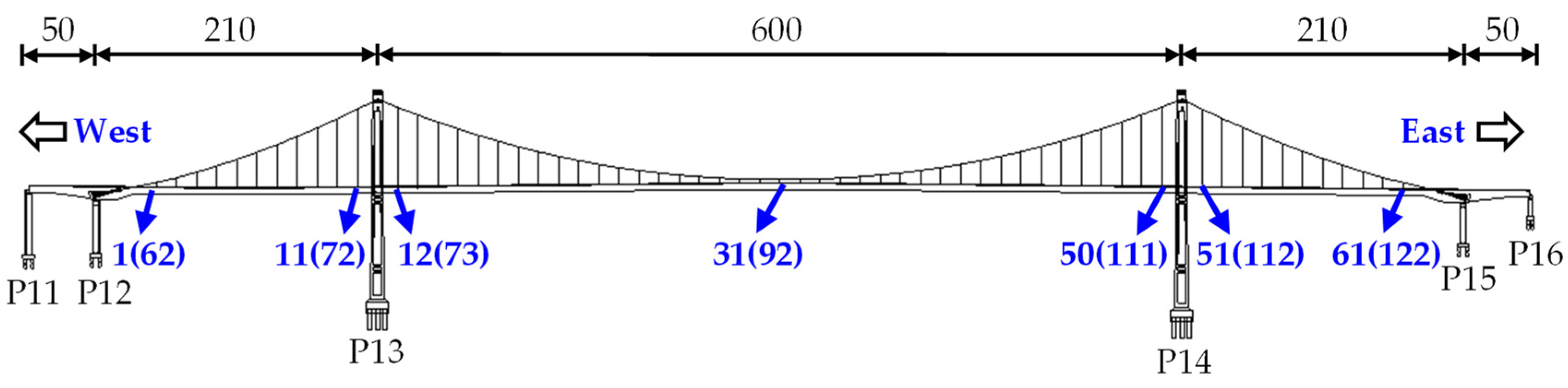
The Egongyan special track bridge is a self-anchored suspension bridge with a main span of 600 m, and it is the world’s largest bridge of its kind, as shown in Figure 5. The main bridge span combination is 50 + 210 + 600 + 210 + 50 = 1120 m: a total of five spans. The total width of the main bridge deck is 22 m. The main beam is a mixed structure of steel box and concrete box. The steel box girder section is 926.4 m long, and the concrete box girder section is 170.16 m long. A steel–concrete joint section with a length of 11.72 m is present at the junction of the steel box and the concrete box on both sides. The steel box adopts six web sections made of Q345qD and Q420qE steel. The concrete box adopts a single-box three-chamber box girder, and it is made of C55 concrete.

The suspension bridge has 122 hangers in total, with 61 hangers on the upstream and downstream sides. A three-dimensional finite element model was built using Midas/civil 2019, which is professional software for bridge structure analysis. The model is divided into 937 nodes and 924 elements (674 beam elements and 250 tension-only elements). The main beams and bridge towers are simulated by beam elements, and the main cables and hangers are simulated by tension-only truss elements (cable elements).

3.2. Setting Damage Scenarios and Building Database

Owing to the joint effects of environmental factors and external loads, damage to the hangers of suspension bridges during operation is mainly manifested in rust or breakage of wires after aging and cracking of the protective sleeve. The corrosion and fracture of the hangers will cause the effective cross-sectional area to decrease. Ignoring the changes in the quality of the entire hanger after the steel wire is corroded and broken, this study adopts a method for reducing the elastic modulus of the hanger to simulate the damage of the hanger. The damage rate is defined to represent the damage severity of the hanger, and the value of the damage rate is the reduction rate of the elastic modulus of the hanger.

For convenience, this article numbers all the hangers according to the following rules. From the west to the east side span, the hangers on the upstream side are sequentially numbered 1, 2, 3... 59, 60, 61, and those at the downstream side are sequentially numbered 62, 63, 64… 120, 121, 122, as shown in Figure 5.

To test the performance of the proposed method, this section identifies the preset single-location damage, multi-location damage, and different damage severities of the hangers. The 1–31 hangers were chosen as the damage object, and the damage scenario was defined as a combination of damage type and degree of damage. There are three types of damages: damage to a single hanger, two hangers, and three hangers. The damage severity was set as 5, 15, 25, 35, and 45%. Therefore, there are 15 damage scenarios in this study, and each scenario corresponds to multiple damage combinations. The specific settings of the damage scenarios are shown in

Table 1. Details of damage scenarios and division of samples.

Scenarios	Damage Types	Damage Severity (%)	Damage Combinations	Training Samples	Validation Samples	Test Samples
1	Single damaged hanger	5	31	327	100	100
2		15	31	327	100	100
3		25	31	327	100	100
4		35	31	327	100	100
5		45	31	327	100	100
6	Two damaged hangers 1	5	36	412	100	100
7		15	36	412	100	100
8		25	36	412	100	100
9		35	36	412	100	100
10		45	36	412	100	100
11	Three damaged hangers 1	5	35	395	100	100
12		15	35	395	100	100
13		25	35	395	100	100
14		35	35	395	100	100
15		45	35	395	100	100
$\Sigma$	/	/	510	5670	1500	1500

¹ The damage of the two hangers can only happen to nine randomly selected hangers, i.e., No. 2, 5, 10, 13, 17, 19, 24, 27, and 30; therefore, the number of corresponding damage combination is $C_9^2$. Moreover, three damages can only occur on hangers No. 5, 10, 13, 17, 19, 24, and 30, and the number of the corresponding damage combination is $C_7^3$.

.

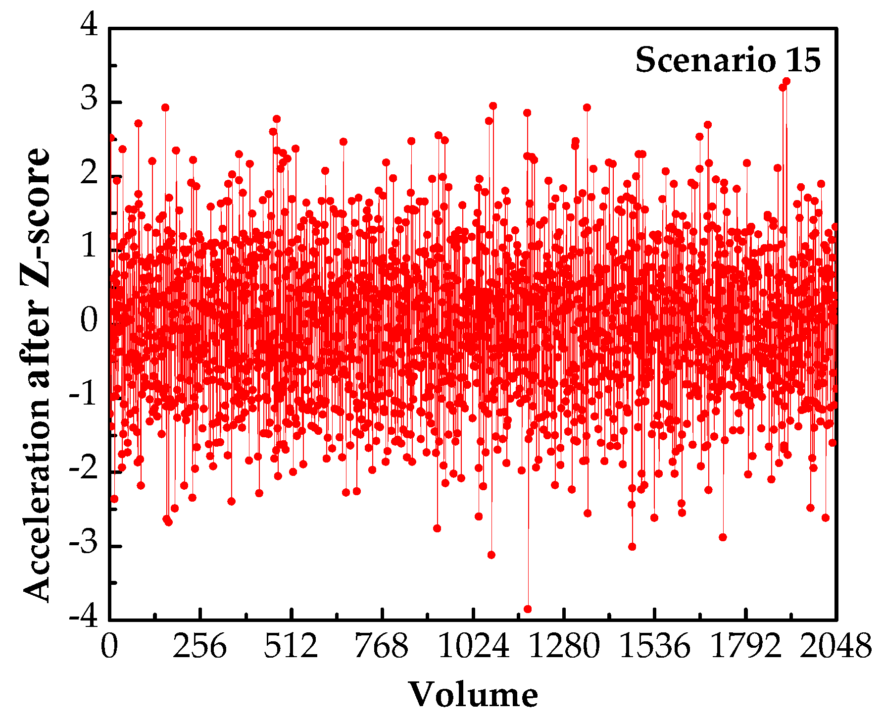
According to the damage scenarios shown in Table 1, the finite element model was subjected to ambient excitation for dynamic analysis, and the vertical acceleration of hangers 1–31 was obtained. The ambient excitation was simulated by white noise excitation with a sampling frequency of 512 Hz, and the analysis time was 34 s. Each damage combination contained 31 acceleration data, and the sequence length of each data was 17,408. The Z-score normalization method was used to preprocess the acquired data. Figure 6 is part of the preprocessed acceleration data of hanger 15 under scenario 15.

The 31 acceleration data collected under the same damage combination are composed of multi-channel data in the order of the hanger number, and a total of 510 acceleration data with a dimension of 17,408 × 31 can be obtained. Then, each piece of acceleration data is divided into 17 samples with dimensions of 1024 × 31, so a total of 8670 samples can be generated from 510 pieces of data. Each sample is marked with the damage location and degree, and all samples constitute the database. Finally, the database is divided into a training set, validation set, and test set, which approximately conforms to the ratio of 6:2:2. The number of samples is shown in Table 1.

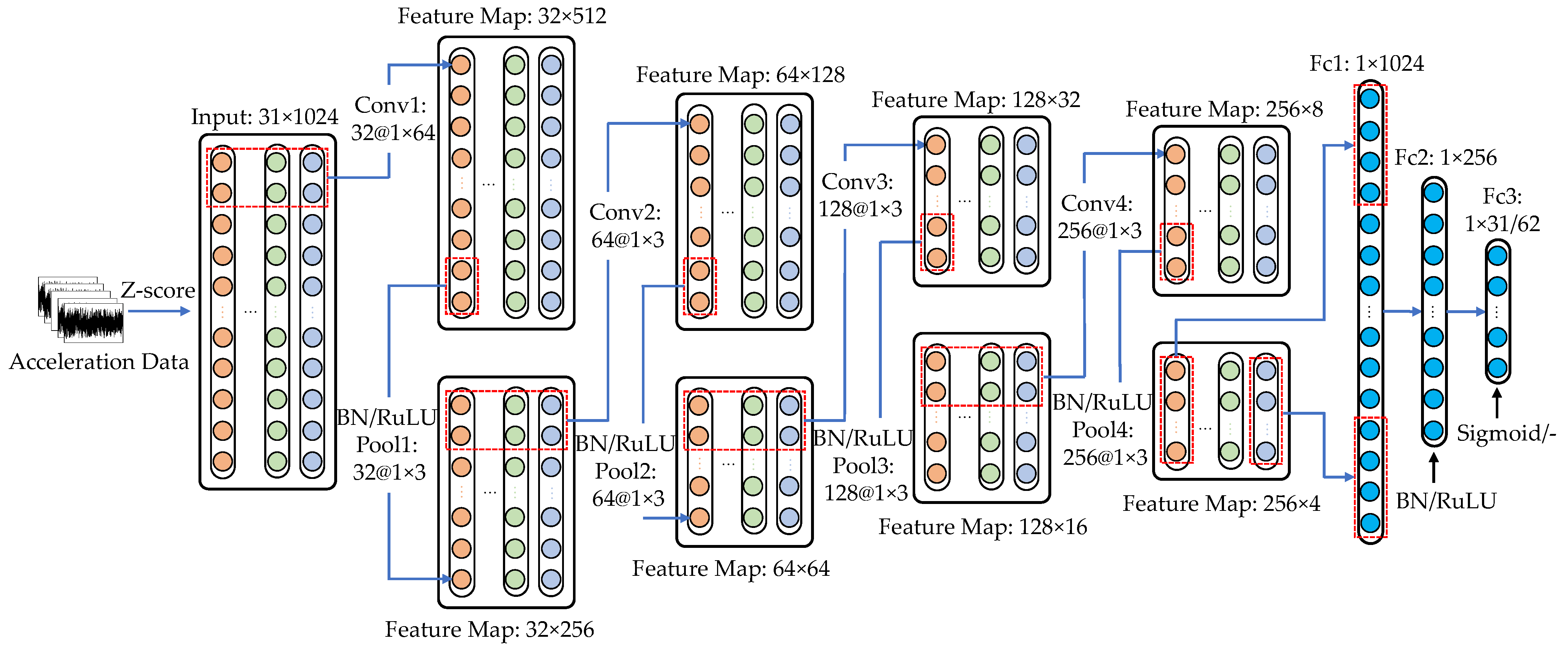
3.3. Architecture of the Proposed CNN-LSTM

A CNN-LSTM for the damage localization and severity prediction of hangers is designed. The architecture of the CNN includes four convolutional blocks for extracting the high-dimensional features of accelerations (denoted as CNN features) and three fully connected layers for damage localization or severity recognition. The architecture of LSTM uses the LSTM layer to extract the time-series features of accelerations (denoted as LSTM features). It should be noted that CNN and LSTM share the three fully connected layers. After merging the extracted CNN and LSTM features, the fused features are used as the input of the fully connected layer to predict the damage location or severity.

The model input adopts the acceleration with dimensions of 1024 × 31, where the input height 31 is the number of hangers, and the input width 1024 is the sequence length. However, the input dimension of the LSTM layer is related to the time step and sequence length. This study sets the input dimension of the LSTM layer to 64 × 496, where 64 is the time step and 496 is the sequence length. Therefore, the sample dimensions need to be converted according to the following steps. Each sample is divided into 16 parts with dimensions of 64 × 31. Then, the 16 parts of the data are spliced along the first dimension into a sequence of 496 acceleration data points, so the transformed sample dimension is 64 × 496.

The LSTM layer consists of 64 LSTM units and 496 hidden neurons. Convolutional blocks are composed of a convolutional layer, a BN layer, an activation function, and a pooling layer. Fully connected block 1 is composed of a fully connected layer and a BN layer, and fully connected block 3 is the classification layer. The size of the convolution kernel in convolutional block 1 is 64 × 1, and the size of the convolution kernel in other convolutional blocks is 3 × 1. The activation function of the convolutional block and the fully connected block 1 selects ReLU. The pooling layer in the convolutional block adopts max pooling with a stride of 2. For the prediction of damage severity, the fully connected block 3 has 31 outputs, corresponding to the number of hangers. For damage localization, each hanger has two states (damaged/undamaged), and the fully connected block 3 has a total of 62 outputs. The architecture of the proposed CNN-LSTM model is shown in Figure 7, and the parameters are shown in

Table 2. Parameters of CNN-LSTM.

Layer		Size/No.	Stride	Padding	Input/Output	Activation
Convolutional block 1	Conv1	64 × 1/32	2	SAME	31 × 1024/32 × 512	ReLU
	BN layer	-	-	-	-	-
	Pool1	3 × 1/32	2	SAME	32 × 512/32 × 256	-
Convolutional block 2	Conv2	3 × 1/64	2	SAME	32 × 256/64 × 128	ReLU
	BN layer	-	-	-	-	-
	Pool2	3 × 1/64	2	SAME	64 × 128/64 × 64	-
Convolutional block 3	Conv3	3 × 1/128	2	SAME	64 × 64/128 × 32	ReLU
	BN layer	-	-	-	-	-
	Pool3	3 × 1/128	2	SAME	128 × 32/128 × 16	-
Convolutional block 4	Conv4	3 × 1/256	2	SAME	128 × 16/256 × 8	ReLU
	BN layer	-	-	-	-	-
	Pool4	3 × 1/256	2	SAME	256 × 8/256 × 4	-
LSTM layer		-	-	-	64 × 496/64 × 256	-
Fully connected block 1	Fc1	-	-	-	1280/1280	-
	BN layer	-	-	-	256/256	ReLU
Fully connected block 2	Fc2	-	-	-	256/31(62)	-
Fully connected block 3	Fc3	-	-	-	31(62)	Sigmoid (-)

Note. The size of the parameter used for damage localization is in brackets, and the size of the parameter used for damage severity prediction is outside the brackets.

.

3.4. Model Training and Hyperparameter Optimization

This study is based on the deep learning framework Pytorch and the programming language Python to complete the model compilation work. A computer with an Intel Core i5-9300H CPU, GeForce GTX 1650 GPU, and RAM 16.00 GBs was used. Additionally, Windows 10, Pytorch 1.4.0, and Python 3.8.2 operating systems were used, as well as CUDA 10.2 software.

For deep learning algorithms, hyperparameters are critical for model performance; therefore, the model parameters need to be adjusted and optimized. The following hyperparameters were optimized and adjusted by the control variable method: learning rate, rate of dropout, mini-batch, and BN layer. The specific parameters to be adjusted are shown in

Table 3. Hyperparameters optimization of CNN-LSTM model.

Parameters to Be Adjusted	Value	Parameters to Be Adjusted	Value
Learning rate	0.01	Mini-batch	32
	0.005		64
	0.001		128
	0.0005	Rate of dropout	0
	0.0001		0.3
BN layer	Setting		0.5
	Not Setting		0.7

. The epoch was set to 50, and the average epoch duration was 9720 s. The damage recognition results of the CNN-LSTM model with different learning rates are plotted in Figure 8. It should be noted that the accuracy is the ratio of the number of samples correctly localized in the validation set. Val-Mse is the mean square error between the prediction vector of the damage severity and the target vector.

Figure 8 indicates that under different learning rates, the loss of CNN-LSTM used for damage localization and severity prediction, respectively, shows a short horizontal segment in the second to eighth epoch, and then, it continues decreasing until the value stabilizes. As shown in Figure 8a, the training speed of the damage localization is the fastest when the learning rate is 0.0001 and 0.0005, and the accuracy is higher under the same epoch, but the accuracy curve with a learning rate of 0.0005 is more volatile. Moreover, Figure 8b shows that when the learning rate is 0.0005, the loss and Val-Mse for predicting damage severity are small. Therefore, the learning rates of the CNN-LSTM model used for damage localization and damage severity prediction were set as 0.0001 and 0.0005, respectively.

The final adjustment result of other hyperparameters is that the convolutional layer and the fully connected layer are added to the BN layer, the mini-batch is 64, and the fully connected layer does not use dropout.

3.5. Damage Localization of Suspension Bridge Hangers

Based on the trained CNN-LSTM model in Section 3.4, the damage location of the test set is predicted. To intuitively display the performance of the proposed method, the number of samples for which the CNN-LSTM model correctly locates the damage in the test set is shown in

Table 4. Test results of CNN-LSTM on damage localization of the hangers.

Scenarios	1	2	3	4	5	6	7	8
No. of samples correctly identified	58	76	95	98	96	97	100	94
Scenarios	9	10	11	12	13	14	15	$\Sigma$
No. of samples correctly identified	100	100	96	100	100	100	100	1410

.

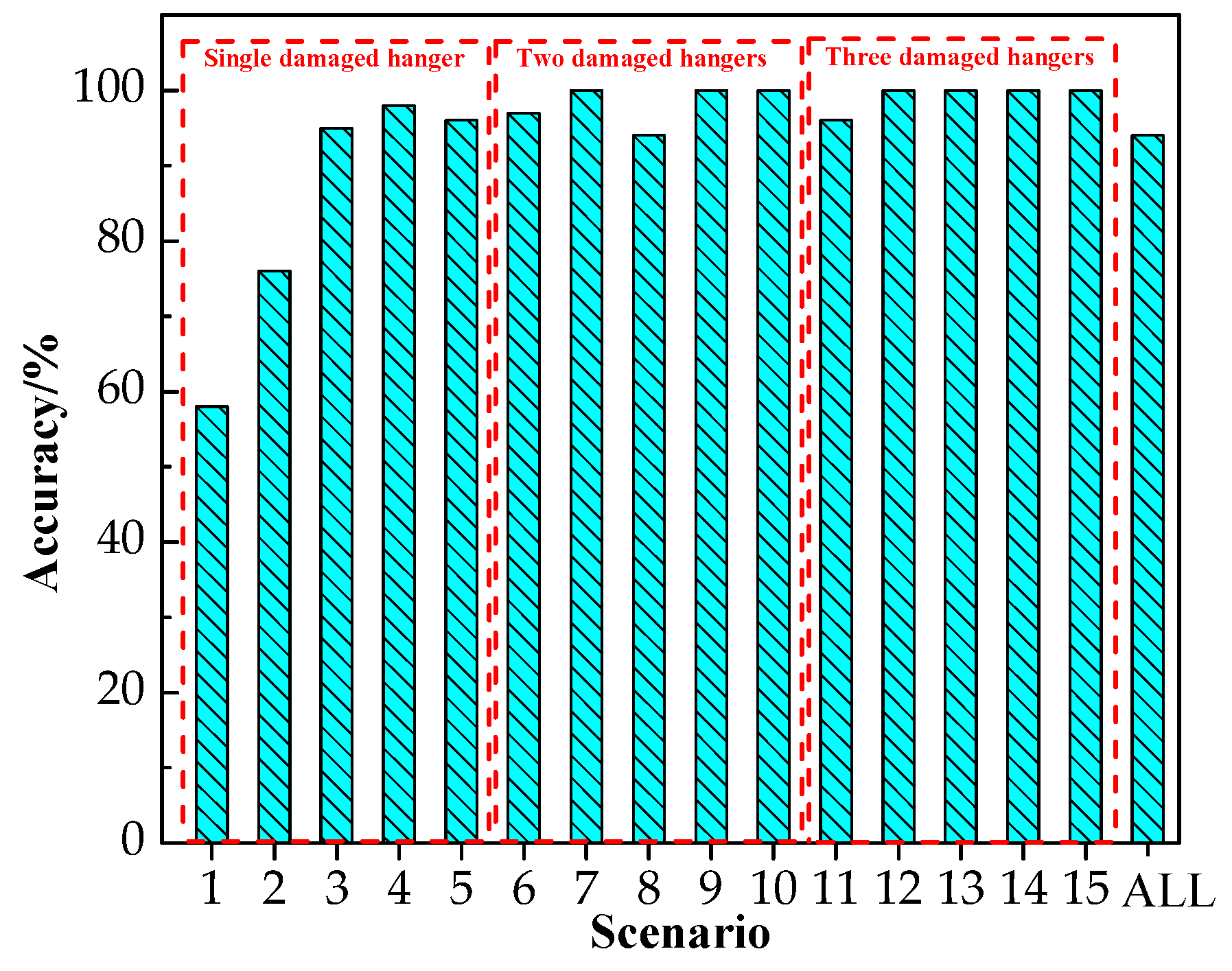
Figure 9 presents the accuracy of the damage localization of hangers under various damage scenarios. “All” in the figure denotes the accuracy of the entire test set, i.e., the average value of scenarios 1–15.

The following can be drawn from Table 4 and Figure 9.

(i)

The accuracy of damage localization of the hangers in the test set reaches 94.0%, showing that the proposed CNN-LSTM can effectively complete the task of damage localization.

(ii)

Comparing the recognition results of different damage scenarios, the accuracy of the CNN-LSTM model in damage localization is between 58.0 and 100%. The accuracy in scenarios 1 and 2 is relatively low, i.e., 58 and 76%, respectively, and the accuracy of the other scenarios remains above 94%. The comparison results show that except for scenarios 1 and 2, the CNN-LSTM-based damage identification method has higher accuracy in locating the damage of hangers.

(iii)

When comparing the recognition results of different damage types, the proposed method has little difference in the accuracy of a single damaged hanger, as well as two and three damaged hangers. The accuracy increases from 84.6 to 99.2%, which is an increase of approximately 15%. From the above results, it can be inferred that the accuracy of the proposed model in damage localization is less affected by the number of damaged hangers.

3.6. Damage Severity Prediction of Suspension Bridge Hangers

The absolute identification error (AIE) of the damage severity of the undamaged and damaged hangers under different damage scenarios is calculated in

Table 5. AIE of the damage severity of hangers under different damage scenarios.

Scenarios			Average AIE of Undamaged Hangers (%)	Average AIE of Damaged Hangers (%)
1	Single damaged hanger	5%	0.229	1.726
2		15%	0.068	2.047
3		25%	0.026	1.711
4		35%	0.017	2.070
5		45%	0.024	2.470
6	Two damaged hangers	5%	0.061	0.648
7		15%	0.005	0.913
8		25%	0.005	1.102
9		35%	0.002	1.159
10		45%	0.010	0.852
11	Three damaged hangers	5%	0.018	0.563
12		15%	0.001	1.006
13		25%	0.001	0.804
14		35%	0.003	1.012
15		45%	0.016	0.405

.

It can be seen from Table 5 that the AIE of damage severity prediction of undamaged hangers based on the CNN-LSTM model is in the range of 0.001–0.229%, where the average AIE of damage scenario 1 is the largest, and those of scenarios 12 and 13 are the smallest. Comparing the AIE of different damage types, the three damaged hangers are the lowest, the two damaged hangers are the second, and the single damaged hanger is relatively high. The AIE of the CNN-LSTM model for predicting the damage severity of damaged hangers is between 0.563 and 2.470%, where the AIE of each scenario of the single damage type is higher than that of the other damage types. According to the above analysis, the proposed model has high accuracy in predicting the severity of the undamaged hangers. The proposed model predicts that the damage severity of the damaged hangers generally performs well, but the prediction result for a single damaged hanger is relatively poor.

To evaluate the performance of the proposed damage identification method, the average relative identification error (ARIE) is used to evaluate the recognition effect of the proposed model on the prediction of the damage severity of hangers, which is expressed as:

$$ARIE={\displaystyle {\sum }_i^n\left|\frac{y_{degpred}-y_{degtarg}}{y_{degtarg}}\right|}\times \frac{100\%}{n}$$

(15)

where $y_{degpred}$ is the prediction vector of damage severity, $y_{degtarg}$ is the target vector, and n is the number of hangers under the corresponding scenarios.

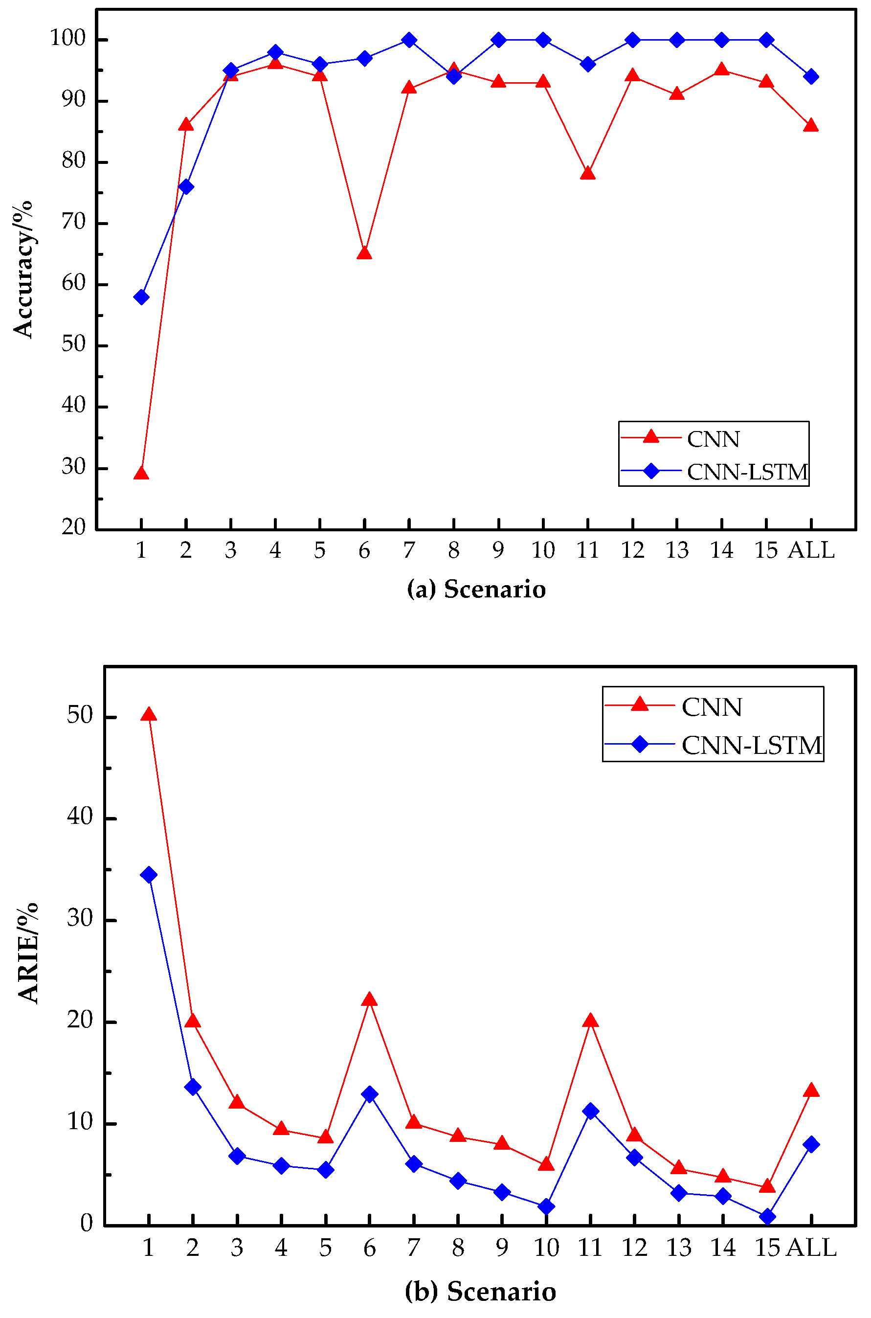
When calculating the ARIE, this study only focuses on the damaged hangers. The value of the evaluation index ARIE is calculated according to Equation (15) and presented in Figure 10.

The following conclusions can be drawn from Figure 10.

(i)

The ARIE of the CNN-LSTM model for the damage severity prediction of hangers is 8.0% in the test set. The ARIE under different damage scenarios is between 0.90 and 34.52%, and the ARIE under most damage scenarios is below 7.0%.

(ii)

For the same damage type, the ARIE decreases as the damage severity increases. The single damage scenarios decrease the fastest, with a decrease of approximately 29.03%, and the two and three damaged scenarios decrease by 11.06 and 10.37%, respectively. It can also be found from the ARIE results of the different damage severities that the CNN-LSTM model has relatively small prediction errors for larger damage severities (≥15%), while the accuracy of damage prediction for smaller damage severities (such as 5%) is poor.

(iii)

For the same damage severity, as the number of damaged hangers increases, ARIE shows an overall downward trend.

4. Discussion

The anti-noise performance of the proposed model in Section 3 will be discussed, and the prediction performance of CNN-LSTM and CNN will be compared in this section.

4.1. Influence of Environmental Noise on the Proposed Method

The bridge structure is in a tough external environment, and the structural response will inevitably be disturbed by environmental factors. Therefore, it is necessary to discuss the anti-noise performance of the proposed CNN-LSTM-based damage identification method under different noise levels. This paper adds noise to the obtained acceleration time-history response according to Equation (16), and the noise level is measured using the signal-to-noise ratio [36].

$$\begin{array}{c}\widehat{x}=x_{signal}+x_{noise}=x_{signal}+\epsilon N\left(\mu ,{\sigma }^2\right)\\ \epsilon =sqrt\left({\displaystyle {\sum }_i^n{x}_i^2}/\left(n\times {10}^{SNR/10}\right)\right)\end{array},$$

(16)

where $\widehat{x}$ and $x_{signal}$ are acceleration samples with and without noise, respectively, SNR is the signal-to-noise ratio, $N\left(\mu ,{\sigma }^2\right)$ is Gaussian noise obeying $\mu =0,{\sigma }^2=1$, and n is the length of the acceleration sample data.

Noise was added to the test samples to obtain five new test sets with signal-to-noise ratios of 20, 10, 6.67, 5, and 3.33, respectively; moreover, the trained CNN-LSTM model (i.e., first training) in Section 3.4 was used for testing. Figure 11 shows the identification results of the damage localization and severity prediction of hangers under different noise levels.

It can be seen from Figure 11 that the damage recognition effect of the CNN-LSTM model on the hangers is greatly affected by environmental noise. In terms of the overall trend, the accuracy of damage localization and the ARIE of the damage severity decreases and increases with the increase in noise level, respectively. When the SNR is 10, the damage localization accuracy can reach approximately 75%, but the ARIE of the severity prediction increases significantly. When the SNR is 3.33, the recognition accuracy is only 46.40%, which is 47.60% lower than the test result without noise, and the ARIE is close to 50%.

The CNN-LSTM model was retrained with a new training set composed of samples with Gaussian noise (SNR: 10, 5, and 3.33) and noise-free samples, and the test set with different noise levels was fed into the retrained model. The test results are shown in Figure 11. It can be seen from Figure 11 that the anti-noise performance of the CNN-LSTM model after retraining with noisy training samples was greatly improved. When the SNR is 5 and 3.33, the accuracy of the damage localization of the hangers is increased by 17.40 and 20.66%, and the ARIE of the severity prediction is reduced by 11.67 and 19.00%, respectively. The results show that using the acceleration response dataset containing noise for the second training of the model can effectively improve the anti-noise performance of the model against higher noise levels. Simultaneously, it also indicates that the proposed model can quickly learn the damage characteristics in the acceleration response with noise and has a strong learning ability.

4.2. Performance Comparison

Based on the time series modeling ability of LSTM, this paper combines it with CNN for damage identification, obtaining promising results. However, it is essential to compare the performance of the CNN-LSTM model against the CNN model to further verify the merit of this research. The architecture of the corresponding CNN model is presented in Figure 12, and the detailed parameters of such a model are tabulated in

Table 6. Parameters of the corresponding CNN model.

Layer		Size/No.	Stride	Padding	Input/Output	Activation
Convolutional block 1	Conv1	64 × 1/32	2	SAME	31 × 1024/32 × 512	ReLU
	BN layer	-	-	-	-	-
	Pool1	3 × 1/32	2	SAME	32 × 512/32 × 256	-
Convolutional block 2	Conv2	3 × 1/64	2	SAME	32 × 256/64 × 128	ReLU
	BN layer	-	-	-	-	-
	Pool2	3 × 1/64	2	SAME	64 × 128/64 × 64	-
Convolutional block 3	Conv3	3 × 1/128	2	SAME	64 × 64/128 × 32	ReLU
	BN layer	-	-	-	-	-
	Pool3	3 × 1/128	2	SAME	128 × 32/128 × 16	-
Convolutional block 4	Conv4	3 × 1/256	2	SAME	128 × 16/256 × 8	ReLU
	BN layer	-	-	-	-	-
	Pool4	3 × 1/256	2	SAME	256 × 8/256 × 4	-
Fully connected block 1	Fc1	-	-	-	1024/1024	-
	BN layer	-	-	-	256/256	ReLU
Fully connected block 2	Fc2	-	-	-	256/31(62)	-
Fully connected block 3	Fc3	-	-	-	31(62)	Sigmoid (-)

Note. The size of the parameter used for damage localization is in brackets, and the size of the parameter used for damage severity prediction is outside the brackets.

. The training set, validation set, and test set of these two models come from the database established in Section 3.2.

Figure 13 shows a comparison of the damage recognition results between the CNN-LSTM model and the CNN model.

As shown in Figure 13, compared to the CNN-based damage identification method, the overall recognition accuracy of the damage localization based on the CNN-LSTM model increases by 8.13%, and the ARIE of severity prediction decreases by 5.20%.

5. Conclusions

A new method of bridge damage identification combining CNN and LSTM is proposed. The proposed method uses LSTM to extract the time-series features of the acceleration data, which are merged with the high-dimensional features of the acceleration data extracted by CNN to realize bridge damage localization and severity prediction. A finite element model was employed to simulate the damage of the hangers of a large-span suspension bridge, and the acceleration dataset was obtained by time-history response analysis to verify the effectiveness and accuracy of the proposed model. The following work was carried out:

(1)

A database containing 8670 damage samples was constructed and divided into a training set, validation set, and test set. Afterward, the training set and the validation set were used to train and select the proposed CNN-LSTM model. For the entire test set, the accuracy of the damage localization of hangers reached 94.00%, and the ARIE of the damage severity prediction was just 8.00%.

(2)

To study the noise immunity of the proposed method, noise with different signal-to-noise ratios was added to the samples in the database, and then the CNN-LSTM model was retrained, and the test set after adding noise was predicted. The results show that when the SNR is 3.33, the accuracy of damage localization reached 67.06%, and the ARIE of the damage severity identification was 31%.

(3)

The performance improvement of the CNN-LSTM model was investigated. The damage recognition performances of the CNN and CNN-LSTM models were compared and analyzed. The results show that the accuracy of damage localization based on CNN-LSTM increased by 8.13%, and the ARIE of the damage severity prediction decreased by 5.20% compared with CNN.

From the above results, it could be concluded that the proposed method can accurately realize the identification of different damage locations and degrees of the target hangers. However, this method may possess a poorer recognition effect on the hangers with minor damage. Therefore, it is indispensable to improve the recognition effect of minor damages in the future. In addition, the main factor that affects the accuracy of the model is the similarity between the training set and the actual situation. As a result, more data under different scenarios will be collected in the future, which is expected to further improve the accuracy of the model.