
Optimization of the Weighted Multi-Facility Location Problem Using MS Excel


1
Department of Logistics, University of Defence, Kounicova 65, 662 10 Brno, Czech Republic
2
Department of Intelligence Support, University of Defence, Kounicova 65, 662 10 Brno, Czech Republic
3
Department of Quantitative Methods, University of Defence, Kounicova 65, 662 10 Brno, Czech Republic
4
Department of Fire Support, University of Defence, Kounicova 65, 662 10 Brno, Czech Republic
*
Author to whom correspondence should be addressed.
Algorithms 2021, 14(7), 191; https://0-doi-org.brum.beds.ac.uk/10.3390/a14070191
Submission received: 12 May 2021
/
Revised: 18 June 2021
/
Accepted: 23 June 2021
/
Published: 25 June 2021
(This article belongs to the Special Issue Metaheuristic Algorithms and Applications)
Abstract
:This article presents the possibilities in solving the Weighted Multi-Facility Location Problem and its related optimization tasks using a widely available office software—MS Excel with the Solver add-in. To verify the proposed technique, a set of benchmark instances with various point topologies (regular, combination of regular and random, and random) was designed. The optimization results are compared with results achieved by a metaheuristic algorithm based on simulated annealing principles. The influence of the hardware configuration on the performance achieved by MS Excel Solver is also examined and discussed from both the execution time and accuracy perspectives. The experiments showed that this widely available office software is practical for solving even relatively complex optimization tasks (Weighted Multi-Facility Location Problem with 100 points and 20 centers, which consists of 40 continuous optimization variables in two-dimensional space) with sufficient quality for many real-world applications. The method used is described in detail and step-by-step using an example.
1. Introduction
“Computers have the potential to turn the biggest math-phobe into a math user, if not a lover” wrote Andrew Vázsonyi in his book Which Door has the Cadillac Adventures of a Real-Life Mathematician [1].
The aim of this work is to find a way to solve the Multi-Facility Location Problem (MFLP) with available hardware and software and to design a simple and understandable method that’s usable in practice. We do not focus on the fastest solutions to very complex problems; we verify the proposed method (in the supplementary file) on data files corresponding to the real needs of experts in the field of logistics and perform calculations on personal computers. The first experiments to solve the MFLP problems in this way were investigated in [2] and it was proven that the results obtained on the applied benchmarks were sufficiently accurate for practical use.
We believe that the availability and ease of use of our method will support many of those who are interested in solving these types of tasks. To enable the improvement and optimization of our method, in addition to its description, we also designed test tasks suitable for their own experiments. The attached file also provides an example of how to use this method (available for download at suplementary).
To approach the practice, in this work we examine the possibility of solving Weighted MFLP problems, where the criterion of distance optimization is corrected by weights, which corresponds to, for example, the amount of material, the frequency of dispensing and more. In this work we refer to it as MFLP-W.
The article is organized as follows. The rest of this section reviews the literature concerning this topic and presents the aim of this work in detail along with the MFLP-W problem formulation. Section 2 describes the methods used. In Section 3, the three types of benchmark tasks (one is designed for the possibility of calculating the optimal value, the other is partially created by generating random values, the third is generated completely randomly) are presented, together with the optimization results obtained using the evolutionary method of the MS Excel Solver and with their comparison with the results of a metaheuristic method—simulated annealing. Each task is solved on three different hardware (HW) configurations by repeating the calculations a hundred times. The obtained results are statistically evaluated and graphically presented mainly in the form of histograms. Section 4 provides the discussion and concludes this article.
1.1. Literature Review
There are a number of sources in the literature dealing with various types of tasks related to logistics and the use of heuristics algorithms in their solution. Resources focused on the multi-facility and single-facility location problem are important for our work.
In [3] is presented a simple and effective Genetic Algorithm for the two-stage capacitated facility location problem (TSCFLP). The TSCFLP is a typical location problem that arises in freight transportation. In this problem, a single product must be transported from a set of plants to meet customers’ demands, passing out by intermediate depots. The objective is to minimize the operation costs of the underlying two-stage transportation system thereby satisfying the demand and capacity constraints of its agents. For this purpose, a genetic algorithm is proposed.
In paper [4] a new hybrid optimization method called the Hybrid Evolutionary Firefly-Genetic Algorithm is proposed, which is inspired by the social behavior of fireflies and the phenomenon of bioluminescent communication. The method combines the discrete Firefly Algorithm with the standard Genetic Algorithm.
In [5] is described a Multiple Ant Colony System to solve the Single Source Capacitated Facility Location Problem (SSCFLP). Lagrangian heuristics have been shown to produce good solutions for the Single Source Capacitated Facility Location Problem. A hybrid algorithm, which combines Lagrangian heuristics and the Ant Colony System, is developed for the SSCFLP.
In [6] a discrete version of particle swarm optimization (DPSO) is employed to solve an uncapacitated facility location problem that is one of the most widely studied in combinatorial optimization. In addition, a hybrid version with a local search is defined to get more efficient results. The results are compared with a continuous particle swarm optimization (CPSO) algorithm and two other metaheuristics studies, namely, genetic algorithm and evolutionary simulated annealing.
In [7] is proposed a novel model for the reliable facility location problem. Instead of assuming the allocation of a fixed number of facilities to each customer as in the existing works, there is set the number of allocated facilities as an independent variable in the proposed model, which makes the model closer to real-life scenarios but more difficult to be solved by traditional methods. To handle it, EAMLS is proposed. This is a hybrid evolutionary algorithm, which combines a memorable local search (MLS) method and an evolutionary algorithm (EA).
Article [8] is focused on the capacitated Multi-Facility Weber problem with rectilinear, Euclidean, squared Euclidean and lp distances. This problem deals with locating m capacitated facilities in the Euclidean plane so as to satisfy the demand of n customers at the minimum total transportation cost. The location and the demand of each customer is known and the transportation cost is proportional to the distance and the amount of flow between customers and facilities. Three new heuristic methods are presented, each of which is based on one of the three well-known metaheuristic approaches: simulated annealing, threshold accepting, and genetic algorithms.
Paper [9] is focused on a new variant of the problem known as Single-Source Capacitated Multi-Facility Weber Problem, also known as continuous location–allocation problem, entails determining the locations of a predefined number of facilities in a planar space and their related customer allocations. To tackle the problem efficiently and effectively, an iterative two-phase heuristic algorithm is put forward. This algorithm produces superior results when assessed against the proposed simulated annealing algorithm.
In article [10] an extension of the multi-Weber facility location problem is proposed with a rectilinear-distance in the presence of passages over a non-horizontal line barrier. For testing purposes, a benchmark is used based on the transformation of the main problem into an equivalent p-median problem. Experimental results evidence the efficiency and validity of the proposed heuristics, which are capable of obtaining high-quality solutions within acceptable computation times.
Based on the Plant Growth Simulation Algorithm (PGSA), study [11] proposed an intelligence optimization algorithm for solving facility location problems. This compared the calculating results of PGSA with the Genetic Algorithm (GA) for a distribution center location problem, and from the result, it was observed that PGSA is better than GA on accuracy.
Study [12] investigates the capacitated planar multi-facility location-allocation problem by considering various capacity constraints. The performance of the proposed greedy randomized adaptive search procedure is tested using benchmark data sets from literature. The computational experiments show that the proposed methods provide encouraging solutions.
The MFLP-W and related problems can be applicable in areas such as logistics, engineering, transportation, planning and scheduling, computer science, supply chains and many others. Foltin et al. [13] shows future logistics applications in the military; they discuss the planning process and its subsequent implementation to ensure logistical support to deployed units and propose discrete event simulation for professional training.
Another example where the MFLP is used is the Tactical Decision Support System (TDSS). This system was developed to support commanders in their decision-making processes [14]. This system is composed of a number of models of military tactics for optimization of the operational task at hand, see, for example, [15,16,17,18,19,20].
MFLP problem solving described in the literature uses proprietary software or specialized platforms. There is no use of ordinary office software.
1.2. Main Aim of This Work
The article discusses the use of commercial Excel software (SW) to solve the MFLP problem with weights of existing facilities (MFLP-W). It explains the method used and the benchmarks on which it is verified. Plane coordinates and the calculation of distances in a Euclidean space are used in the calculations. The calculated data should therefore be considered approximate and serve mainly as a basis for further decisions. Optimization calculations in MS Excel are compared with the results obtained using the simulated annealing method.
In this research we use three benchmarks with the same difficulty (100 points and 20 centers), but different topology. The first benchmark is designed for the possibility of calculating the optimal solution, the others are created using a random number generator. The results obtained by the calculations in the Excel environment are compared with the results obtained by the calculations using the metaheuristic method (simulated annealing). The tasks are solved on three HW configurations, to verify the influence of the hardware configuration on the accuracy of the calculations.
Excel software and its Solver add-in are commercial products. This work does not examine the algorithm used by the Solver add-in. From the point of view of this research, it is a “black box” for which the inputs, settings of basic parameters and outputs are known.
Our method uses office software (Excel with Solver add-in) for solving a Multi-Facility Location Problem with weighted existing facilities, as it is formulated in Section 1.3. The use of the proposed procedure will allow the required calculations to be performed on a personal computer with commonly available office software. No special competencies are required; user-level knowledge is sufficient. Because we hope that the availability of our solution will inspire users to improve the method, in addition to its description, we offer the benchmarks for possible experiments.
1.3. Problem Formulation
There are p points where the coordinates of their positions are known, every point has a weight. The objective is to find the positions of the c centers so that the sum of the distances multiplied by weights (weighted distance) between all the centers and their assigned points will be minimal. Each point will be assigned to exactly one center which is closest to it. Variable c is an integer greater than or equal to 1 and p is an integer greater than or equal to c.
A practical example is a company with a number of existing branches which needs to set up a number of centers that will provide services to these branches. Branches have different supply requirements. The locations of the branches are known; the centers will be built as new. The location of these centers and the branches they will serve are not specified.
The mathematical formulation of this problem is as follows. Let be a set of points (); the coordinates of these points are known. Let be a set of centers (; the coordinates of these points are not known as they are the subject of the optimization. Let every P have a weight .
The Euclidean distance between a center and any point in a two-dimensional space is calculated according to Equation (1). In general, any space, number of dimensions and distance function can be used.
where is the distance between center and point , , are coordinates of the center , and , are coordinates of point .
The objective function of the MFLP-W problem is shown in Equation (2). It corresponds to the sum of weighted distances between all points and their assigned centers which are closest to them.
The optimization goal is in Equation (3); the aim is to find the locations of c centers so that the objective function D is minimal. In the case of two-dimensional space, there are 2c continuous optimization variables.
2. Materials and Methods
For calculations, both a common office notebook designed for administrative work and powerful personal computers used for more demanding calculations and simulations were used. All computers have the Windows 10 operating system and the Office suite installed. These are easily accessible devices that do not require any special knowledge or equipment.
2.1. Evolutionary Method Excel-Solver
The evolutionary algorithms (EAs) are subset of Evolutionary Computations and belongs to a set of modern heuristics-based search methods. Due to the flexible nature and robust behavior inherited from Evolutionary Computation, it is an efficient means of problem-solving for widely used global optimization problems. It can be used successfully in many applications of high complexity [21].
In this work, the results were obtained using an evolutionary method. This method is available in the Solver add-on and is intended for solving a non-continuous problem. It uses genetic algorithms to find “good” solutions to continuous optimization problems. It relies in part on random sampling. It is a nondeterministic method that can provide different solutions in different runs.
According to [22], evolutionary algorithms can be described by means of the following main features.
In the first step, a random selection of samples is performed. The evolutionary algorithm maintains a population of candidate solutions. Only one (or several, with the same goals) of them is the “best”, but other members of the population are “role models” in other areas of the search space where a better solution can be found later. The evolutionary algorithm regularly makes random changes or mutations in one or more members of the current population, resulting in a new candidate solution (which may be better or worse than existing members of the population). The evolutionary algorithm attempts to combine elements of existing solutions in order to create a new solution with some features of each “parent”. Elements of existing solutions are combined in a crossover operation. In the end, the evolutionary algorithm performs a selection process in which the “most suitable” members of the population survive and the “least suitable” ones are excluded. In a limited optimization problem, the term “fitness” depends partly on whether the solution is feasible (i.e., whether it meets all the constraints) and partly on the value of its objective function. The selection process is a step that leads the evolutionary algorithm to ever better solutions.
The algorithm can be presented in this pseudocode notation.
START
Generate the initial population
Compute fitness
REPEAT
Population
Mutation
Crossover
Selection
Compute fitness
UNTIL population has converged
STOP
Convergence values, mutation frequency, base file size, random number, and maximum time without enhancement can also be set for this method. What the effect is of changes in these parameters on the calculation is not stated; therefore, default values were left for all calculations. The default values of parameters are listed in Table 1.
In the attached file (the link for download is in Section 1), the method is described in detail on the example of an MFLP-W task with 25 points and 5 centers.
2.2. Metaheuristic Algorithm
The metaheuristic method is used in order to compare the performance of MS Excel when solving the continuous multi-variable optimization problem. As this metaheuristic method, the simulated annealing-based algorithm is adapted for the MFLP-W problem. This choice was based on our previous experiences in using this method for position optimization problems. The algorithm was implemented by the authors in C++ programming language under the Visual Studio IDE. The concept of this method is inspired by annealing in metallurgy. See [2] for more information.
The basic steps of this method in pseudocode are as follows:
- Generate random solution.
- Set temperature to its maximum limit.
- Repeat points 4 to 6 for a predefined number of times.
- Transform current solution.
- Replace the current solution by the transformed solution with the probability given by the Metropolis criterion.
- Save the best solution if found.
- Cool the temperature.
- When the temperature is not below its lower limit, repeat the whole process in point 3.
- Terminate the algorithm and return the best solution found.
The transformation of the current solution in point 4 is based on changing one randomly selected variable using a random number generator with normal distribution. The size of the change depends on the current value of temperature. The higher the temperature, the bigger the change; this principle allows for the extensive search in the state space at the beginning of the optimization and small tuning near its end. This transformed solution replaces the original with the probability given by the Metropolis criterion in Equation (4). If the transformed solution is better than the original, it is always replaced; otherwise, it depends on the temperature and the difference in solution qualities.
where is the probability that the current solution is replaced by the transformed solution, is the objective function of the current (original) solution, is the objective function of the transformed solution, is the current value of temperature.
The cooling schedule in point 7 is performed according to Equation (5), where is the cooling coefficient ().
3. Performance Evaluation
In this section, results obtained by the benchmark calculations are analyzed. For a better understanding, the terms and abbreviations used are explained in Table 2 and Table 3.
3.1. Hardware and Software Configuration
Hardware configurations. Calculations were performed on three computers with different hardware configurations:
- HW 1-CPU: AMD A10-9620P RADEON R5 2.50 GHz; memory 8.00 GB RAM.
- HW 2-CPU: INTEL CORE i7-7700 3.60 GHz; memory 32.00 GB RAM.
- HW 3-CPU: INTEL CORE i9-9900K 3.60 GHz; memory 32.00 GB RAM.
Software configuration. A 64-bit operating system, Windows 10 Enterprise LSTC, MS Excel 2016, 64 bit, part of the Microsoft Office Suite, with the Solver add-in installed, which performs calculations. In the basic version it allows only one method of calculation using evolutionary algorithms. The Excel environment is used to enter data, calculate intermediate results, and display the result of the entire process.
3.2. Benchmark Instances
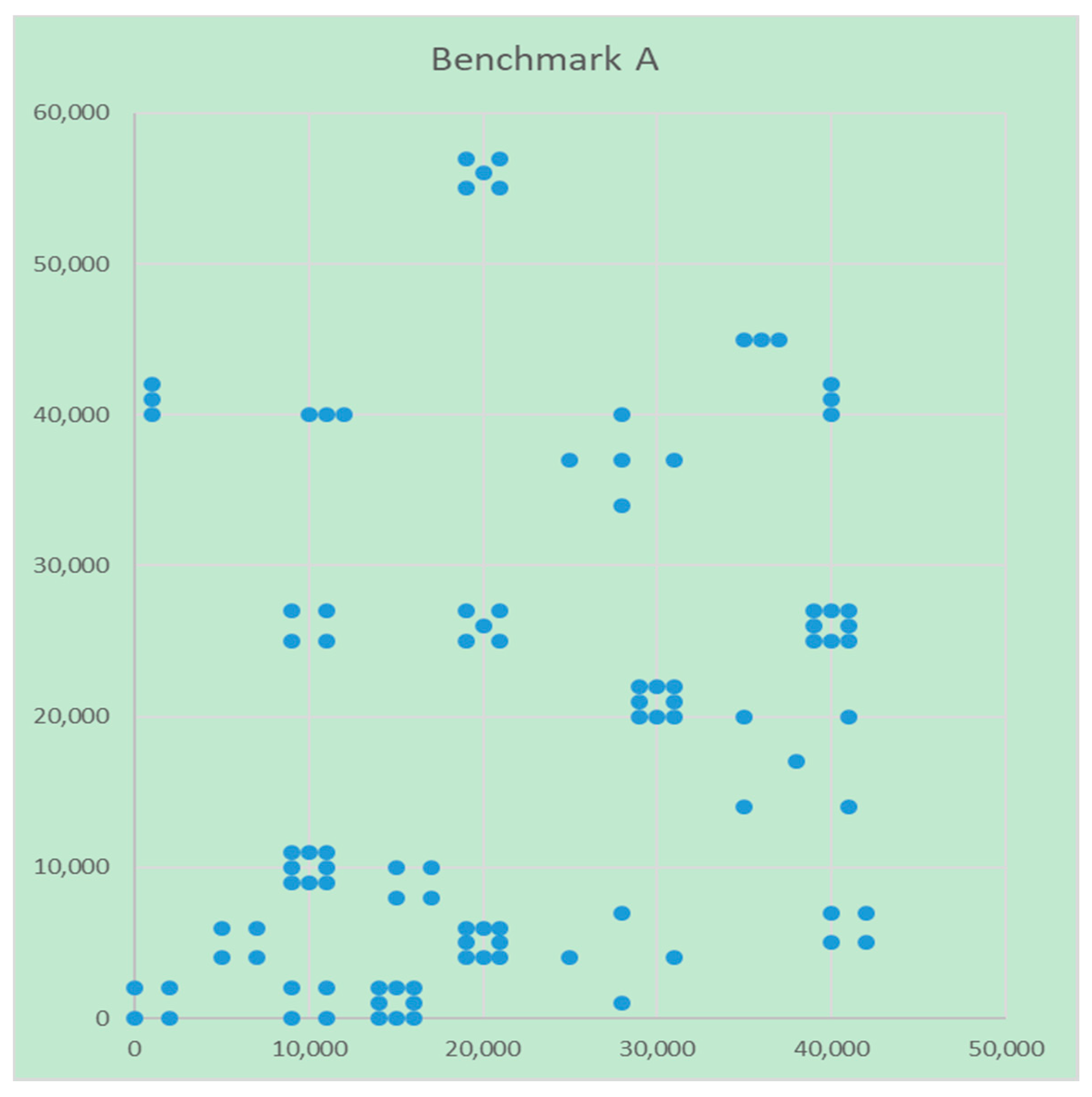
The MFLP-W task calculations will be performed on three benchmarks. The topology of points for the artificial benchmark A (Figure 1) are designed and weighted in a special way, so that it is possible to calculate the optimal solution as the reference value.
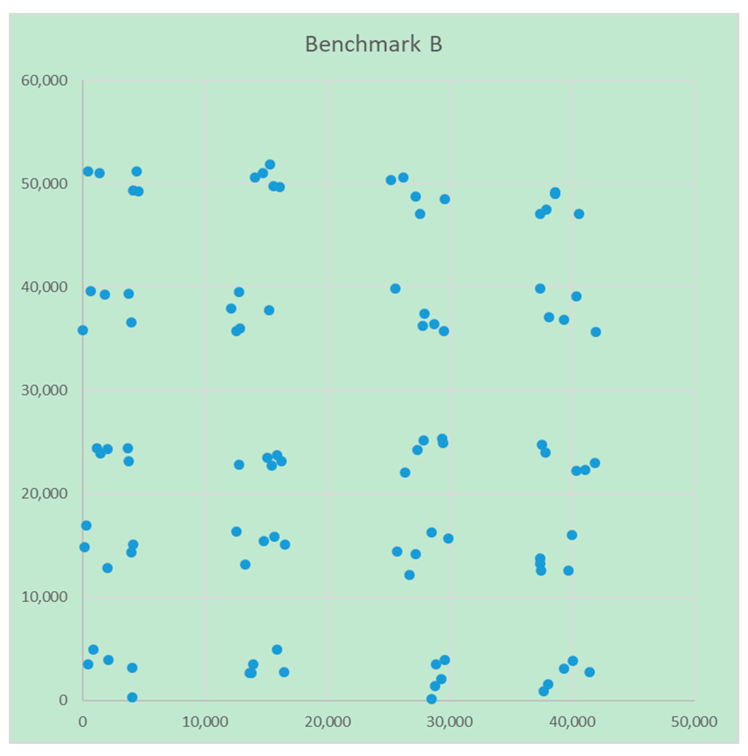
Benchmark B is a combination of twenty randomly generated groups of five points, their position in the area is designed so that there is no mutual influence (Figure 2). The optimal center positions cannot be directly calculated. For benchmark B, the reference value was obtained in three ways:
- Each group is solved separately by an evolutionary method in Excel as a Single Facility Location Problem (SFLP) task. The sum of the resulting values is then the solution of the MFLP problem with this topology (best result 360,186.787);
- The lowest value of 300 calculations by the metaheuristic method on three hardware configurations (the best result 360,186.7863)—as this method provided the best solution, it serves as a reference value.
For benchmark C, values of positions of points are generated by the Excel RANDBETWEEN function in the range 0 to 45,000 for x coordinate, range 0 to 60,000 for y coordinate, for weight in range 1 to 25 (Figure 3). For benchmark C, the reference solution is calculated using the metaheuristic method: the lowest value of 300 calculations on three HW configurations is used. Table 4 shows the reference values for the benchmark instances.
For each benchmark task, 100 optimizations were performed both in the Excel-Solver software (see Section 2.1 for details) as well as using the metaheuristic algorithm (see Section 2.2 for details).
Each task is solved in six ways (thus, in total, 1800 optimizations trials are performed):
- by Excel-Solver evolutionary method on HW1;
- by Excel-Solver evolutionary method on HW2;
- by Excel-Solver evolutionary method on HW3;
- by metaheuristic algorithm on HW1;
- by metaheuristic algorithm on HW2;
- by metaheuristic algorithm on HW3.
For each task, method and hardware configuration, the following parameters and outputs calculated from all individual solutions are recorded:
- minimal solution;
- average solution;
- standard deviation;
- coefficient of variation;
- difference between the reference and the minimal solutions in percent;
- difference between the reference and the average solutions in percent;
- histogram, classes are from 1 percent to 10 percent deviation from reference;
- graph with coordinates for result for the reference and the minimal solution.
3.3. Results
Table 5, Table 6, Table 7, Table 8, Table 9 and Table 10 record the results of the calculations of benchmark instances A, B, C obtained by evolutionary and metaheuristic methods on HW1, HW2 and HW3. The results are also presented in the form of histograms and graphs in Section 3.3.1, Section 3.3.2, Section 3.3.3.
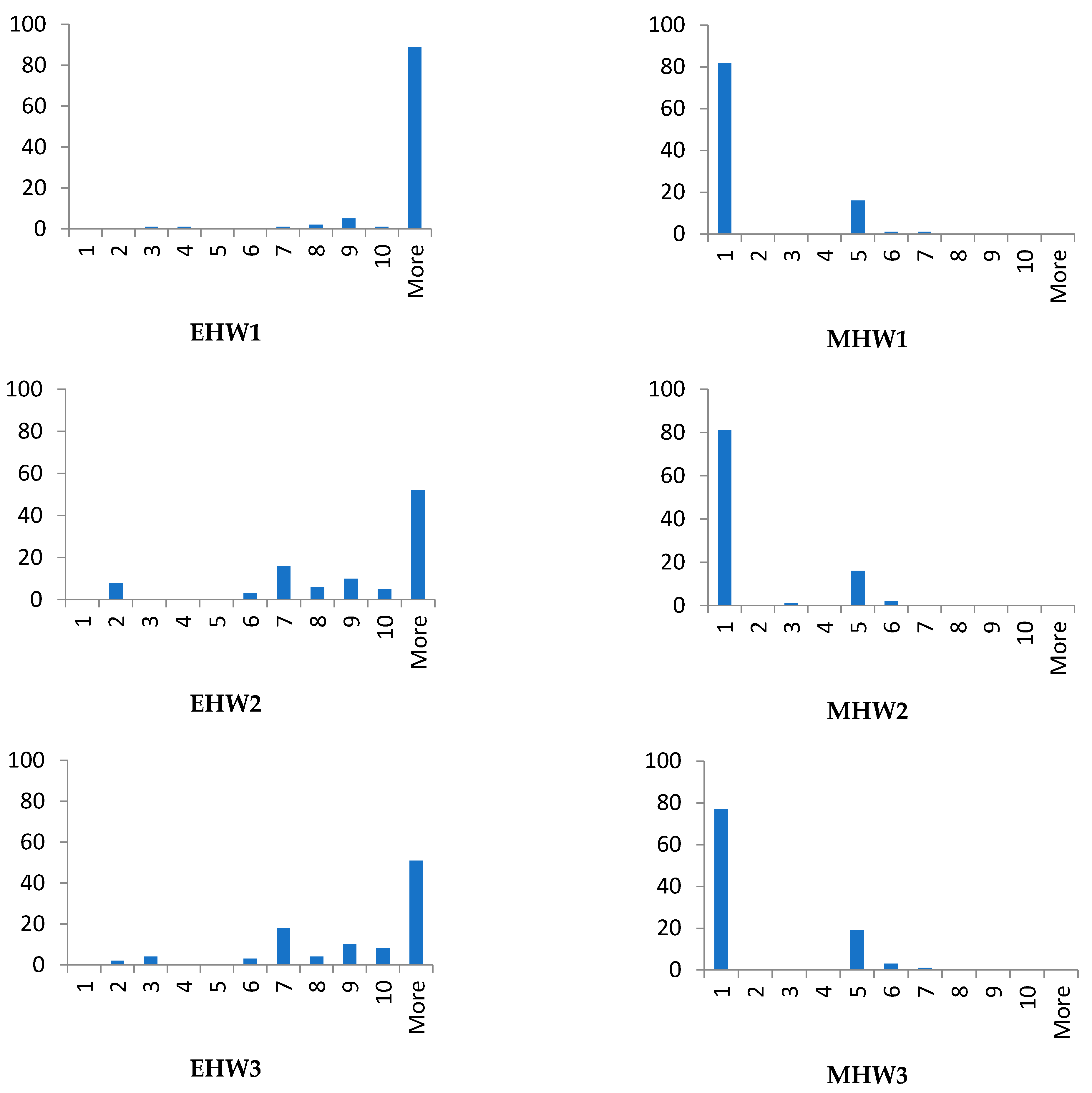
In each method, 100 different results were obtained for benchmarks A, B, and C; the difference between the minimal and the reference values are statistically evaluated using histograms. The intervals are designed in the range of 1–10% of the reference value. The histogram shows the frequency of occurrence of the obtained values in each interval. From the graphs it is possible to assess how accurate the method and influence of the hardware is, see Figure 4, Figure 5 and Figure 6.
3.3.1. Histograms and Solutions for Benchmark A
From the data given in Table 5, Table 6, Table 7, Table 8, Table 9 and Table 10 and on the histograms for benchmark A (see Figure 4), the influence of the used method and hardware configuration can be deduced. Unlike the metaheuristic method, the results of the evolutionary method depend on the performance of the hardware. The metaheuristic algorithm is often very close to the optimum value; however, in a minority number of cases it remained stuck in some local optima.
3.3.2. Histograms and Solutions for Benchmark B
The results of the comparison of the used methods, similarly to benchmark A, show that the accuracy of the metaheuristic method is better in comparison with the evolutionary method, where again the influence of the hardware used for the calculations is significant. In this case (benchmark B), the evolutionary algorithm often finds a solution at the local minimum. The histograms in Figure 5 also show the effects of topology on the results in comparison with benchmark A.
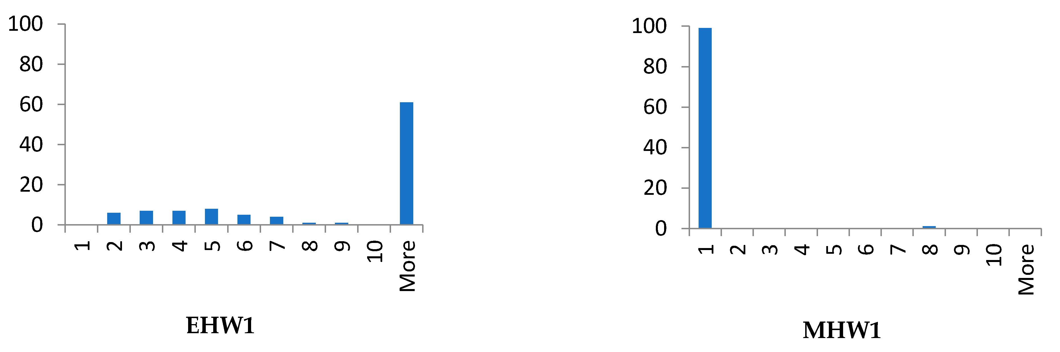
3.3.3. Histograms and Solutions for Benchmark C
The results for benchmark C show that, for randomly distributed points in the plane, the results of the evolutionary algorithm are better than benchmark A. In this case, it can be again stated the positive effect of powerful hardware, on which the optimizations were calculated with the evolutionary algorithm. The hardware configuration has no effect on the performance of the metaheuristic algorithm, only on the optimization time, see Table 11.
3.3.4. Other statistical values for the Evolutionary and Metaheuristic method
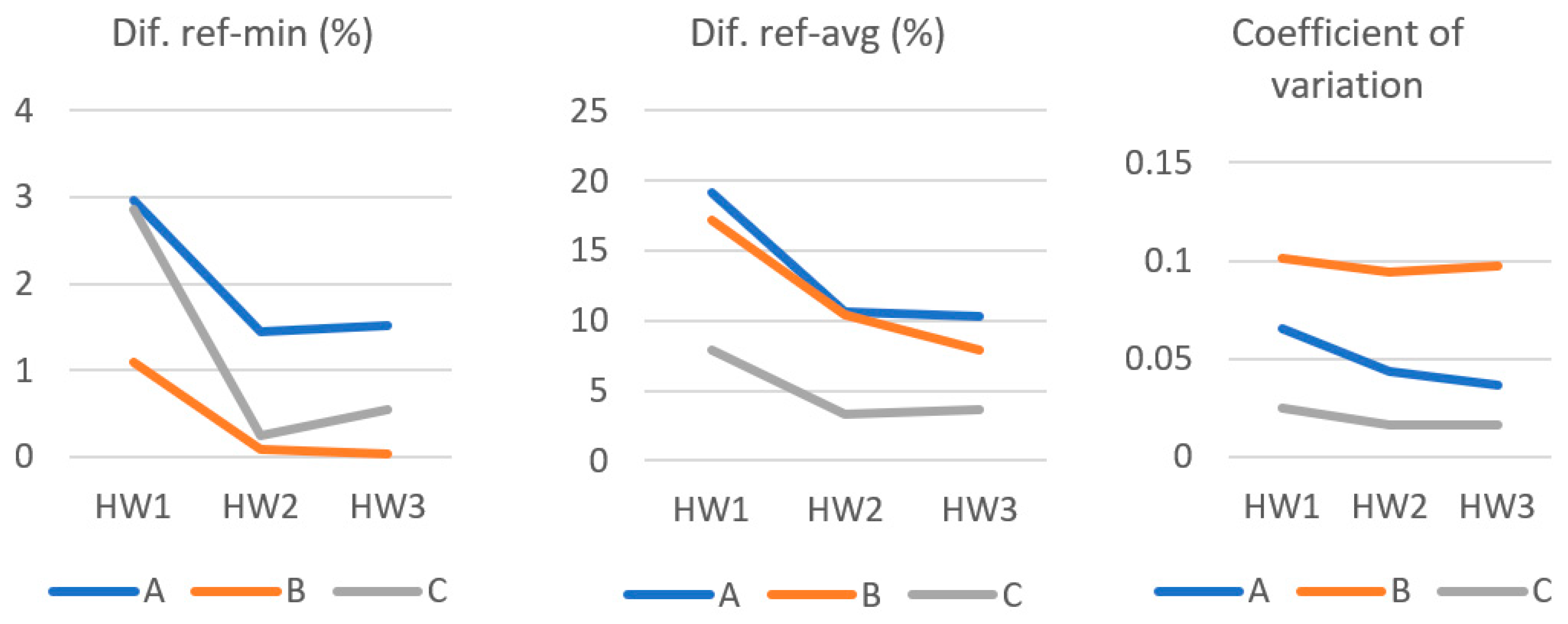
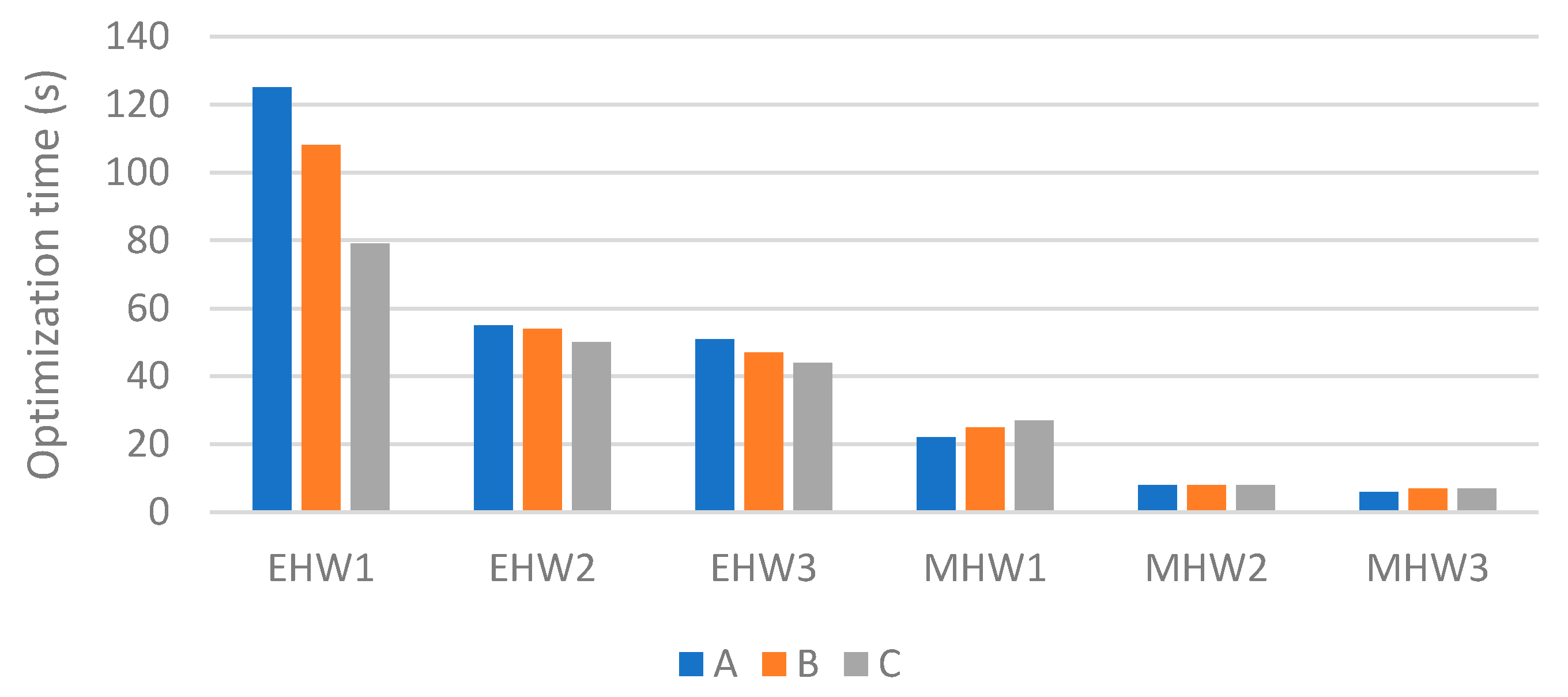
The influence of benchmark topologies and hardware (only for evolutionary algorithm) on selected parameters (Dif. ref-min (%), Dif. ref-avg (%) and coefficient of variation) can be seen in Table 12, Table 13 and Table 14, and in the graph in Figure 7. The last monitored parameter is the average optimization time in Table 15 and Figure 8.
Based on the results of 100 repetitions of calculations on three benchmarks, it can be stated that the evolutionary method depends on the hardware on which the optimizations are performed. The difference between average values and the reference values ranges from 3.7% to 19.2%. The smallest values are for benchmark C. The coefficient of variation describing the variability of the results ranged from 0.016 to 0.101. The smallest values were again reached for benchmark C.
The difference of the minimal values and reference values is more important for practical use. For the evolutionary method it ranges from 0.04% to 2.97%, depending on the hardware and the topology of benchmarks.
4. Discussion and Conclusions
In this work, we extended our research [2] into the possibility of solving MFLP using the available procedures and resources. We focused on extending the MFLP task by weight and examined the effect of the benchmark topology and hardware used for the calculations. All benchmarks have the same complexity in terms of the number of points and centers.
Benchmark A was used in the first phase to verify the accuracy of the method used. It is specially designed to contain several types of groups of points of different sizes, and it is possible to calculate the optimal value for it. The obtained results met expectations.
Benchmark B was designed as a semi-artificial one, consisting of 20 groups of five randomly generated points with weights. The groups are artificially arranged so that there can be no interaction at the values of the weights used. Such a topology corresponds to a situation in practice where there are several corporate branches in large cities. The correctness of the method used was confirmed again.
Benchmark C was created completely using a random number generator. Both positions and point weights are generated. Additionally, in this case, the results were in line with expectations.
Histograms are chosen as a suitable way to evaluate the obtained data. In addition to the already known fact that the results obtained by the metaheuristic algorithm are orders of magnitude better, it is possible to observe the influence of topology. Thus, the assumption that the topology does not significantly affect the result was not confirmed.
The histograms also show the effect of the HW configuration on the overall performance of MS Excel Solver. On HW1, the results are visibly worse than on HW2 and HW3. Results on HW2 and HW3 are comparable as these configurations are similar; they differ in the CPU type only, not in CPU frequency or installed memory.
The tables and graphs in Part 3.6 show the importance of repeating calculations using the evolutionary method. While the difference between the average and reference value is around 10% for high-performance hardware, the difference between the minimum and reference value is less than 1%.
Supplementary Materials
The following are available online at https://0-www-mdpi-com.brum.beds.ac.uk/article/10.3390/a14070191/s1.
Author Contributions
Conceptualization, P.N., M.B. and M.P.; methodology, P.N. and P.S.; software, P.N. and P.S.; validation, P.N. and J.N.; formal analysis, P.N.; investigation, P.N.; resources, P.N.; data curation, P.N. and P.S.; writing—original draft preparation, P.N. and P.S.; visualization, P.N.; supervision, P.S.; project administration, P.N.; funding acquisition, P.N. All authors have read and agreed to the published version of the manuscript.
Funding
This research received no external funding.
Data Availability Statement
Not applicable.
Conflicts of Interest
The authors declare no conflict of interest.
References
- Vazsonyi, A. Which Door Has the Cadillac: Adventures of a Real-Life Mathematician; Writers Club Press: Bloomington, IN, USA, 2002. [Google Scholar]
- Němec, P.; Stodola, P. Optimization of the Multi-Facility Location Problem Using Widely Available Office Software. Algorithms 2021, 14, 106. [Google Scholar] [CrossRef]
- Fernandes, D.R.M.; Rocha, C.; Aloise, D.; Ribeiro, G.M.; Santos, E.M.; Silva, A. A Simple and Effective Genetic Algorithm for the Two-Stage Capacitated Facility Location Problem. Comput. Ind. Eng. 2014, 75, 200–208. [Google Scholar] [CrossRef]
- Rahmani, A.; MirHassani, S.A. A Hybrid Firefly-Genetic Algorithm for the Capacitated Facility Location Problem. Inf.Sci. 2014, 283, 70–78. [Google Scholar] [CrossRef]
- Chen, C.-H.; Ting, C.-J. Combining Lagrangian Heuristic and Ant Colony System to Solve the Single Source Capacitated Facility Location Problem. Transp. Res. Part E Logist. Transp. Rev. 2008, 44, 1099–1122. [Google Scholar] [CrossRef]
- Guner, A.R.; Sevkli, M. A Discrete Particle Swarm Optimization Algorithm for Uncapacitated Facility Location Problem. J. Artif. Evol. Appl. 2008, 2008, 861512. [Google Scholar] [CrossRef] [Green Version]
- Zhang, H.; Liu, J.; Yao, X. A Hybrid Evolutionary Algorithm for Reliable Facility Location Problem. In Parallel Problem Solving from Nature–PPSN XVI. PPSN 2020. Lecture Notes in Computer Science; Bäck, T., Preuss, M., Deutz, A., Wang, H., Doerr, C., Emmerich, M., Trautmann, H., Eds.; Springer: Cham, Switzerland, 2020; Volume 12270. [Google Scholar] [CrossRef]
- Aras, N.; Yumusak, S.; Altmel, I.K. Solving the Capacitated Multi-Facility Weber Problem by Simulated Annealing, Threshold Accepting and Genetic Algorithms. In Metaheuristics, Operations Research/Computer Science Interfaces Series; Doerner, K.F., Gendreau, M., Greistorfer, P., Gutjahr, W., Hartl, R.F., Reimann, M., Eds.; Springer: Boston, MA, USA, 2007; Volume 39. [Google Scholar] [CrossRef]
- Manzour-al-Ajdad, S.M.H.; Torabi, S.A.; Eshghi, K. Single-Source Capacitated Multi-Facility Weber Problem—An Iterative Two Phase Heuristic Algorithm. Comput. Oper. Res. 2012, 39, 1465–1476. [Google Scholar] [CrossRef]
- Amiri-Aref, M.; Shiripour, S.; Ruiz-Hernández, D. Exact and Approximate Heuristics for the Rectilinear Weber Location Problem with a Line Barrier. Comput. Oper. Res. 2021, 132, 105293. [Google Scholar] [CrossRef]
- Tong, L.; Wang, Z.-T. Application of Plant Growth Simulation Algorithm on Solving Facility Location Problem. Syst. Eng. Theory Pract. 2008, 28, 107–115. [Google Scholar] [CrossRef]
- Luis, M.; Ramli, M.F.; Lin, A. A Greedy Heuristic Algorithm for Solving the Capacitated Planar Multi-Facility Location-Allocation Problem. AIP Conf. Proc. 2016, 1782, 040010. [Google Scholar] [CrossRef]
- Foltin, P.; Vlkovský, M.; Mazal, J.; Husák, J.; Brunclík, M. Discrete Event Simulation in Future Military Logistics Applications and Aspects. In Privacy Enhancing Technologies; Metzler, J.B., Ed.; Springer: Berlin/Heidelberg, Germany, 2018; Volume 10756, pp. 410–421. [Google Scholar]
- Stodola, P.; Mazal, J. Tactical Decision Support System to Aid Commanders in their Decision-Making. In Proceedings of the Modelling and Simulation for Autonomous Systems, Rome, Italy, 15–16 June 2016; pp. 396–406. [Google Scholar]
- Stodola, P.; Drozd, J.; Šilinger, K.; Hodický, J.; Procházka, D. Collective Perception Using UAVs: Autonomous Aerial Reconnaissance in a Complex Urban Environment. Sensors 2020, 20, 2926. [Google Scholar] [CrossRef] [PubMed]
- Blaha, M.; Šilinger, K. Application support for topographical-geodetic issues for tactical and technical control of artillery fire. Int. J. Circuits Syst. Signal Process. 2018, 12, 48–57. [Google Scholar]
- Hošková-Mayerová, Š.; Talhofer, V.; Otřísal, P.; Rybanský, M. Influence of Weights of Geographical Factors on the Results of Multicriteria Analysis in Solving Spatial Analyses. ISPRS Int. J. Geo-Inf. 2020, 9, 489. [Google Scholar] [CrossRef]
- Mazal, J.; Rybanský, M.; Bruzzone, A.G.; Kutěj, L.; Scurek, R.; Foltin, P.; Zlatník, D. Modelling of the microrelief impact to the cross country movement. Int. Conf. Harb. Marit. Multimodal Logist. Modeling Simul. 2020, 66–70. [Google Scholar] [CrossRef]
- Františ, P.; Hodický, J. Virtual reality in presentation layer of C3I system. In Proceedings of the MODSIM05—International Congress on Modelling and Simulation: Advances and Applications for Management and Decision Making, Proceedings 2005, Melbourne, Australia, 12–15 December 2005; pp. 3045–3050. [Google Scholar]
- Sekelova, M.; Korba, P.; Hovanec, M.; Mrekaj, B.; Oravec, M.; Szabo, S. Options of measuring the work performance of the air traffic controller. In Transport Means 2018; Kaunas University of Technology: Trakai, Lithuania, 2018; pp. 1476–1481. [Google Scholar]
- Vikhar, P.A. Evolutionary Algorithms: A Critical Review and Its Future Prospects. In Proceedings of the 2016 International Conference on Global Trends in Signal Processing, Information Computing and Communication (ICGTSPICC), Jalgaon, India, 22–24 December 2016; IEEE: Piscataway Township, NJ, USA, 2016; pp. 261–265. [Google Scholar] [CrossRef]
- ‘Solver’. Available online: https://www.solver.com/ (accessed on 1 June 2021).
- Byrd, R.H.; Mary, E.; Hribar, M.E.; Nocedal, J. An Interior Point Algorithm for Large-Scale Nonlinear Programming. SIAM J. Optimization 1999, 9, 877–900. [Google Scholar] [CrossRef]
- Gill, P.E.; Murray, W.; Wright, M.H. Practical Optimization; Academic Press: London, UK, 1981. [Google Scholar]
Figure 1.
Benchmark instance A.

Figure 2.
Benchmark instance B.

Figure 3.
Benchmark instance C.

Figure 4.
Histograms—benchmark instance A.

Figure 5.
Histograms—Benchmark instance B.


Figure 6.
Histograms—Benchmark instance C.


Figure 7.
Values of selected parameters—evolutionary method.

Figure 8.
Average optimization time.


Table 1.
Parameters used for optimization in the Excel-Solver.
| Parameter | Value |
|---|---|
| Max time | Unlimited |
| Iterations | Unlimited |
| Constraint precisions | 0.000001 |
| Convergence | 0.0001 |
| Population size | 100 |
| Random seed | 0 |
| Mutation rate | 0.075 |
| Maximum time without improvement | 30 s |
| Max subproblems | Unlimited |
| Maximum feasible solutions | Unlimited |
| Integer optimality | 1% |
Table 2.
Definitions of terms used.
| Name of Term | Explanation |
|---|---|
| Reference | Optimal or reference solution for an instance. |
| Minimal | Minimal value from set of 100 results |
| Average | Average value from set of 100 results |
| Dif. ref-min | Difference between reference and minimal value (%) |
| Dif. ref-avg | Difference between reference and average value (%) |
| Standard dev. | Standard deviation for set of 100 results |
| Coefficient of variation | Relative standard deviation for set of 100 results |
| Avg. time | Average time of computing one result in set of 100 results |
Table 3.
Definitions of abbreviations used.
| Name of Acronym | Explanation |
|---|---|
| EHW1 | Results of operations with evolutionary method on HW1 |
| EHW2 | Results of operations with evolutionary method on HW2 |
| EHW3 | Results of operations with evolutionary method on HW3 |
| MHW1 | Results of operations with metaheuristic algorithm on HW1 |
| MHW2 | Results of operations with metaheuristic algorithm on HW2 |
| MHW3 | Results of operations with metaheuristic algorithm on HW3 |
Table 4.
Benchmark instances—final values.
| Benchmark Instance | Number of Points | Number of Centers | Reference |
|---|---|---|---|
| A | 100 | 20 | 310,048.77 * |
| B | 100 | 20 | 360,186.79 |
| C | 100 | 20 | 3,399,273.00 |
* Confirmed optimum.
Table 5.
Calculations EHW1.
| Benchmark Instance | A | B | C |
|---|---|---|---|
| Reference value | 310,048.77 | 360,186.77 | 3,399,273.00 |
| Minimal | 319,256.49 | 364,155.78 | 3,496,336.34 |
| Average | 369,489.23 | 422,268.28 | 3,666,323.69 |
| Dif. ref-min (%) | 2.97 | 1.10 | 2.86 |
| Dif. ref-avg (%) | 19.17 | 17.24 | 7.86 |
| Standard dev. | 24,062.23 | 42,651.21 | 91,422.78 |
| Coefficient of variation | 0.0651 | 0.1010 | 0.0249 |
Table 6.
Calculations EHW2.
| Benchmark Instance | A | B | C |
|---|---|---|---|
| Reference value | 310,048.77 | 360,186.77 | 3,399,273.00 |
| Minimal | 314,559.20 | 360,530.87 | 3,407,806.82 |
| Average | 343,051.52 | 397,906.86 | 3,513,082.48 |
| Dif. ref-min (%) | 1.45 | 0.10 | 0.25 |
| Dif. ref-avg (%) | 10.64 | 10.47 | 3.35 |
| Standard dev. | 14,906.14 | 37,515.08 | 56,379.08 |
| Coefficient of variation | 0.0435 | 0.0943 | 0.0160 |
Table 7.
Calculations EHW3.
| Benchmark Instance | A | B | C |
|---|---|---|---|
| Reference value | 310,048.77 | 360,186.79 | 3,399,273.00 |
| Minimal | 314,772.06 | 360,344.72 | 3,417,691.86 |
| Average | 341,912.54 | 388,651.12 | 3,524,354.39 |
| Dif. ref-min (%) | 1.52 | 0.04 | 0.54 |
| Dif. ref-avg (%) | 10.28 | 7.90 | 3.68 |
| Standard dev. | 12,411.75 | 37,700.39 | 59,072.10 |
| Coefficient of variation | 0.0363 | 0.0970 | 0.0168 |
Table 8.
Calculations MHW1.
| Benchmark Instance | A | B | C |
|---|---|---|---|
| Reference value | 310,048.77 | 360,186.79 | 3,399,273.00 |
| Minimal | 310,048.77 | 360,186.79 | 3,399,273.00 |
| Average | 312,878.10 | 360,214.37 | 3,420,905.56 |
| Dif. ref-min (%) | 0 | ||
| Dif. ref-avg (%) | 0.91 | 0.01 | 0.64 |
| Standard dev. | 5747.78 | 58.32 | 17,009.00 |
| Coefficient of variation | 0.0184 | 0.0002 | 0.0050 |
Table 9.
Calculations MHW2.
| Benchmark Instance | A | B | C |
|---|---|---|---|
| Reference value | 310,048.77 | 360,186.79 | 3,399,273.00 |
| Minimal | 310,048.77 | 360,186.79 | 3,399,823.32 |
| Average | 312,993.06 | 360,484.42 | 3,419,586.89 |
| Dif. ref-min (%) | 0 | 0.02 | |
| Dif. ref-avg (%) | 0.95 | 0.08 | 0.60 |
| Standard dev. | 5639.52 | 2671.73 | 13,667.40 |
| Coefficient of variation | 0.0180 | 0.0074 | 0.0040 |
Table 10.
Calculations MHW3.
| Benchmark Instance | A | B | C |
|---|---|---|---|
| Reference value | 310,048.77 | 360,186.79 | 3,399,273.00 |
| Minimal | 310,048.77 | 360,186.79 | 3,400,034.97 |
| Average | 313,718.26 | 360,207.91 | 3,422,185.23 |
| Dif. ref-min (%) | |||
| Dif. ref-avg (%) | 1.18 | 0.66 | |
| Standard dev. | 6288.90 | 41.25 | 15,981.47 |
| Coefficient of variation | 0.0200 | 0.0001 | 0.0047 |
Table 11.
Comparation of selected values—evolutionary and metaheuristic method for benchmark C.
| Benchmark Instance | EHW1 | MHW1 |
|---|---|---|
| Dif. ref-min (%) | 2.86 | 0 |
| Dif. ref-avg (%) | 7.86 | 0.64 |
| Coefficient of variation | 0.0249 | 0.0050 |
Table 12.
Dif. ref-min (%).
| Benchmark Instance | A | B | C |
|---|---|---|---|
| EHW1 | 2.97 | 1.10 | 2.86 |
| EHW2 | 1.45 | 0.10 | 0.25 |
| EHW3 | 1.52 | 0.04 | 0.54 |
Table 13.
Dif. ref-avg (%).
| Benchmark Instance | A | B | C |
|---|---|---|---|
| EHW1 | 19.17 | 17.24 | 7.86 |
| EHW2 | 10.64 | 10.47 | 3.35 |
| EHW3 | 10.28 | 7.90 | 3.68 |
Table 14.
Coefficient of variation.
| Benchmark Instance | A | B | C |
|---|---|---|---|
| EHW1 | 0.0651 | 0.1010 | 0.0249 |
| EHW2 | 0.0435 | 0.0944 | 0.0160 |
| EHW3 | 0.0363 | 0.0970 | 0.0168 |
Table 15.
Average optimization time (in seconds).
| Benchmark Instance | A | B | C |
|---|---|---|---|
| EHW1 | 125 | 108 | 79 |
| EHW2 | 55 | 54 | 50 |
| EHW3 | 51 | 47 | 44 |
| MHW1 | 22 | 25 | 27 |
| MHW2 | 8 | 8 | 8 |
| MHW3 | 6 | 7 | 7 |
Publisher’s Note: MDPI stays neutral with regard to jurisdictional claims in published maps and institutional affiliations. |
© 2021 by the authors. Licensee MDPI, Basel, Switzerland. This article is an open access article distributed under the terms and conditions of the Creative Commons Attribution (CC BY) license (https://creativecommons.org/licenses/by/4.0/).
Share and Cite
MDPI and ACS Style
Němec, P.; Stodola, P.; Pecina, M.; Neubauer, J.; Blaha, M. Optimization of the Weighted Multi-Facility Location Problem Using MS Excel. Algorithms 2021, 14, 191. https://0-doi-org.brum.beds.ac.uk/10.3390/a14070191
AMA Style
Němec P, Stodola P, Pecina M, Neubauer J, Blaha M. Optimization of the Weighted Multi-Facility Location Problem Using MS Excel. Algorithms. 2021; 14(7):191. https://0-doi-org.brum.beds.ac.uk/10.3390/a14070191
Chicago/Turabian StyleNěmec, Petr, Petr Stodola, Miroslav Pecina, Jiří Neubauer, and Martin Blaha. 2021. "Optimization of the Weighted Multi-Facility Location Problem Using MS Excel" Algorithms 14, no. 7: 191. https://0-doi-org.brum.beds.ac.uk/10.3390/a14070191
Note that from the first issue of 2016, this journal uses article numbers instead of page numbers. See further details here.