
qRobot: A Quantum Computing Approach in Mobile Robot Order Picking and Batching Problem Solver Optimization

 ,
,
Abstract
:1. Introduction
2. Work Context
3. Quantum Circuits in the NISQ Era
Variational Quantum Eigensolver
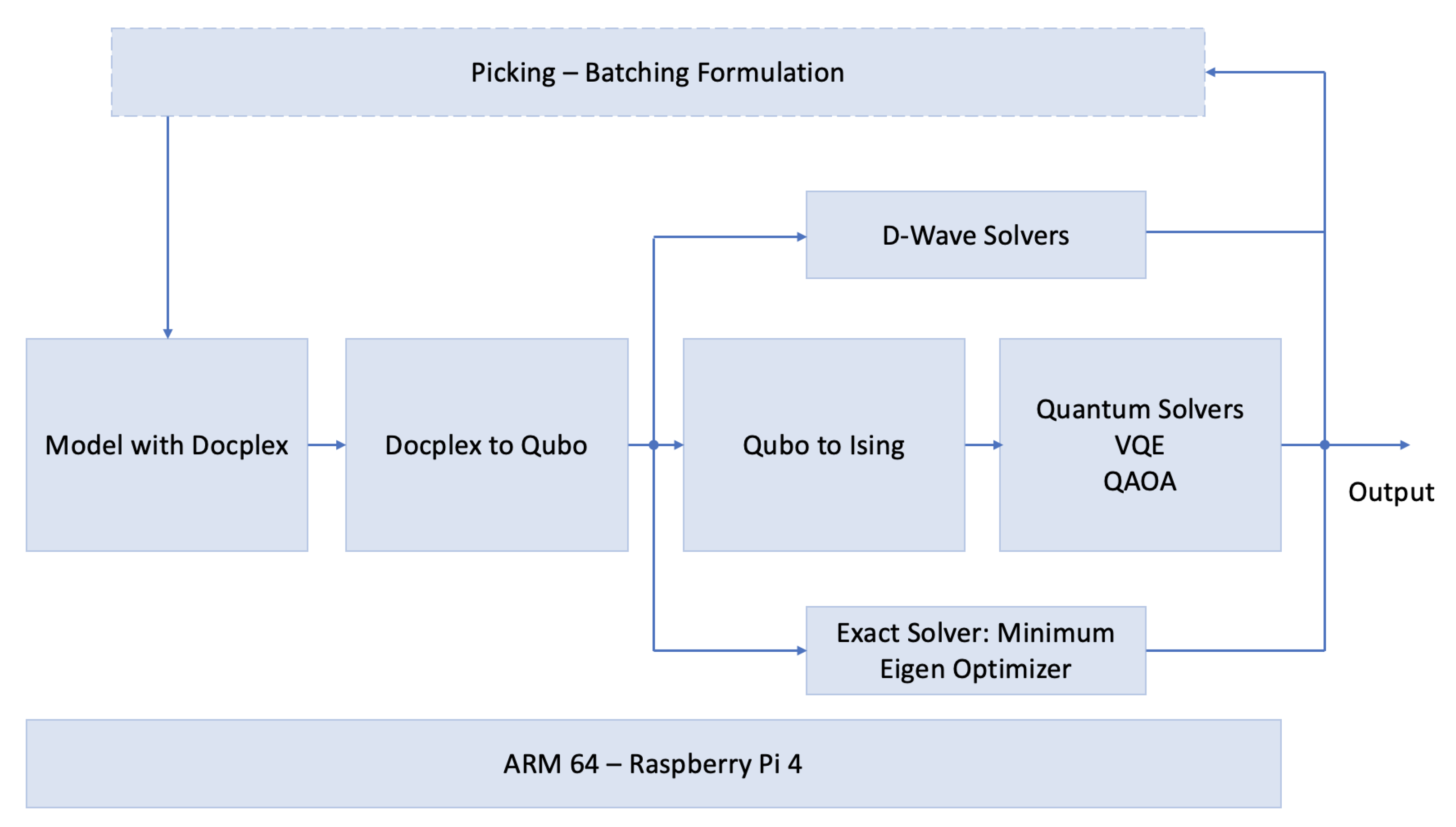
4. Implementation
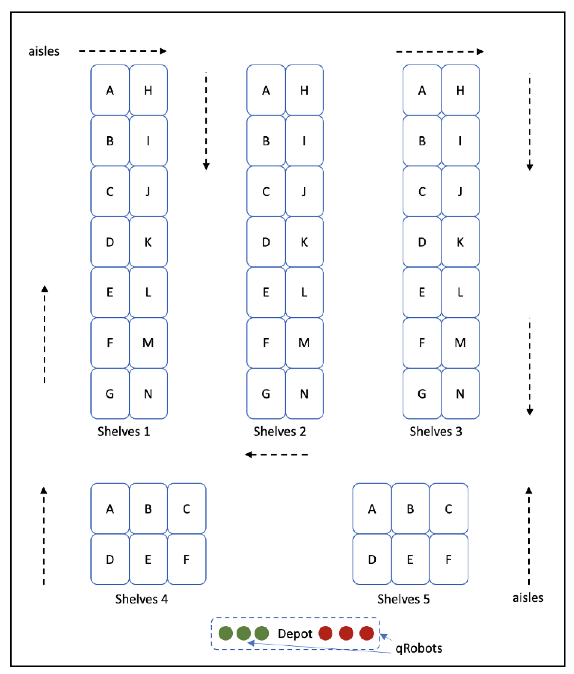
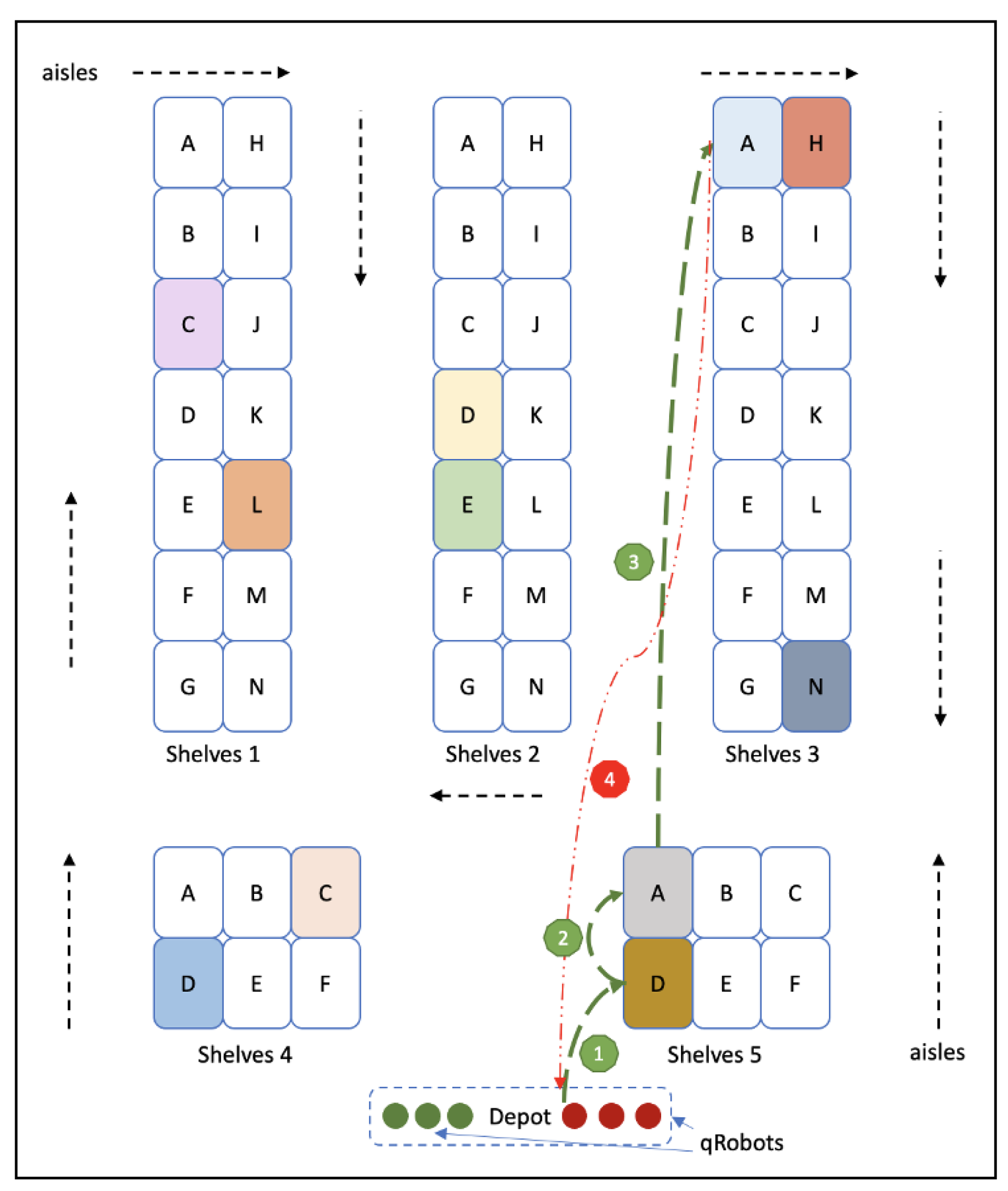
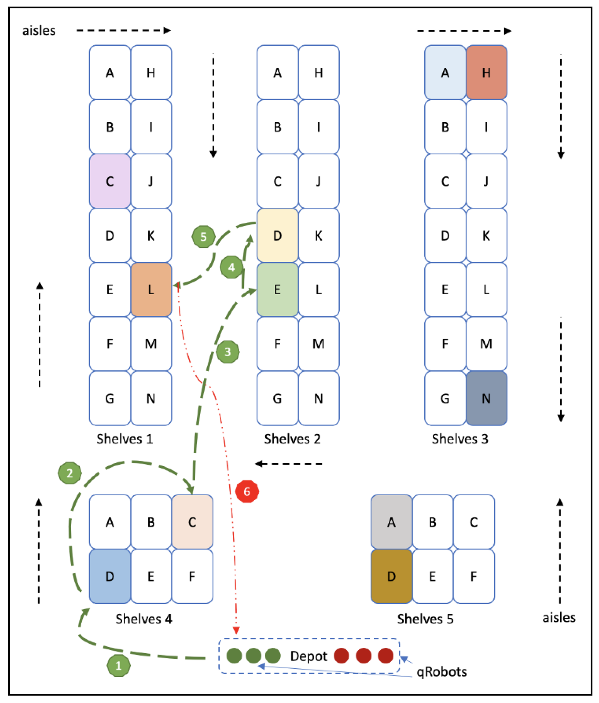
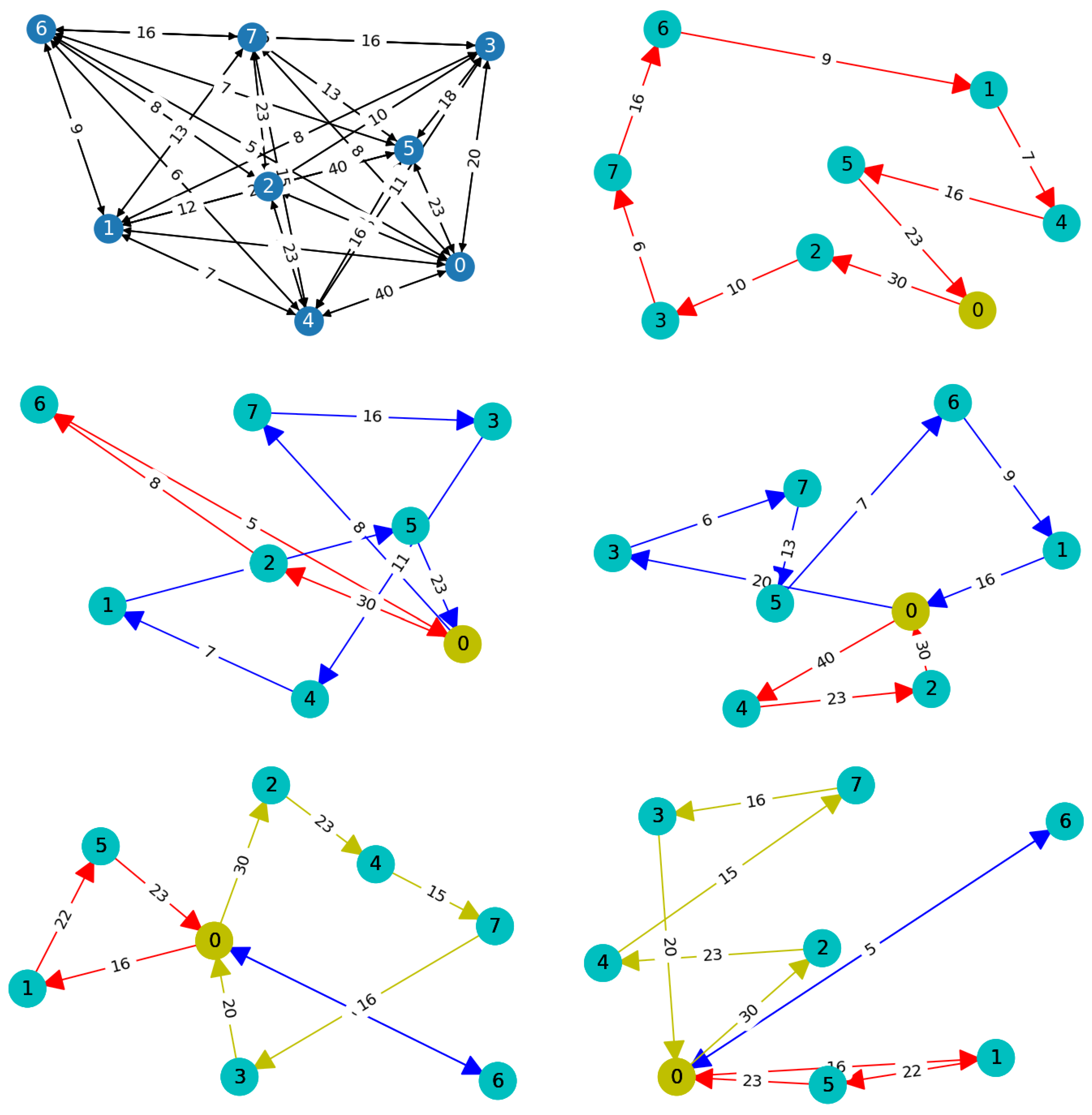
4.1. The Problem’s Formulation
- The strategy we will follow is the picking routing problem to retrieve each lot which the total distance traveled to retrieve all the items in a lot will be calculated.
- For the orders of the storage positions, more than one picking robot can be used.
- Movements in height are not considered.
- Each product is stored in a single storage position, and only one product is stored in each storage position.
- Each picking route begins and ends at the Depot.
- The load capacity for each order will not exceed the load capacity of the picking robot.
- At the moment, the division of order orders is not contemplated. That is, only the batches of closed orders can be prepared.
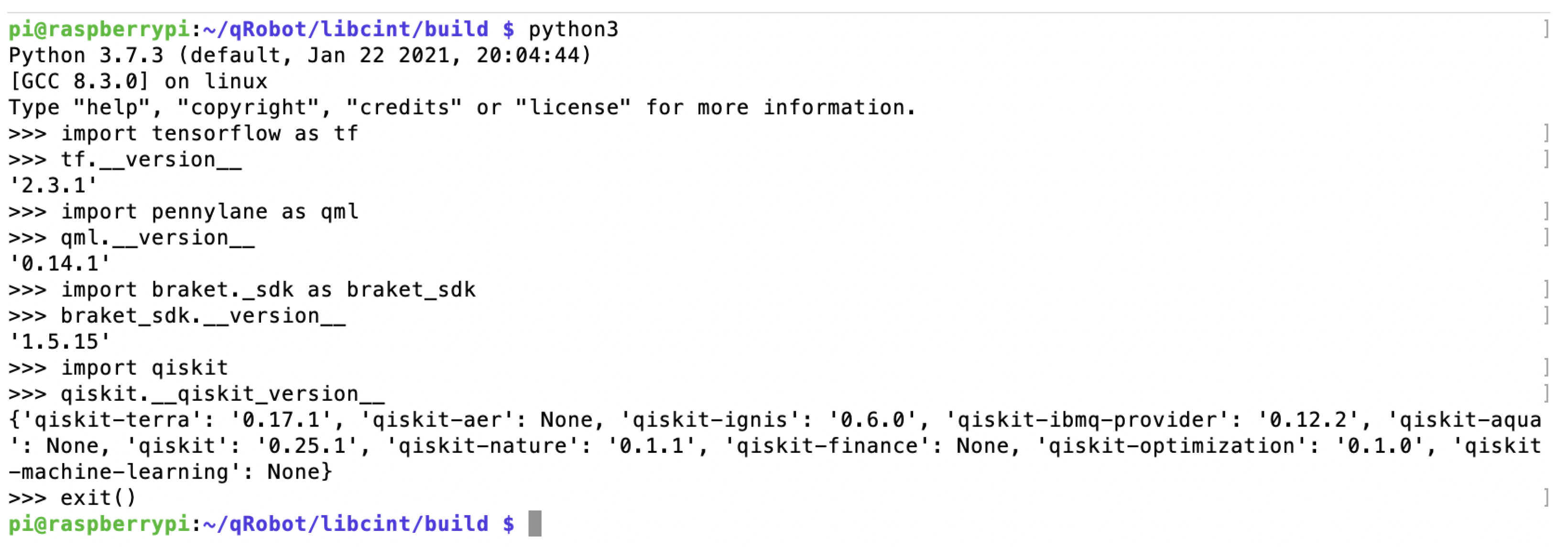
- The concept testing will be done on all AWS-Braket, Pennylane, D-Wave, and Qiskit environments. And we will stick with the scenario that best benefits our proof of concept.
- We will use the docplex [70] to model our formulation.
4.2. Picking and Batching Formulation
4.3. Mapping the Classical to Quantum Optimization
5. Results
6. Discussion
7. Conclusions and Further Work
Author Contributions
Funding
Institutional Review Board Statement
Informed Consent Statement
Data Availability Statement
Acknowledgments
Conflicts of Interest
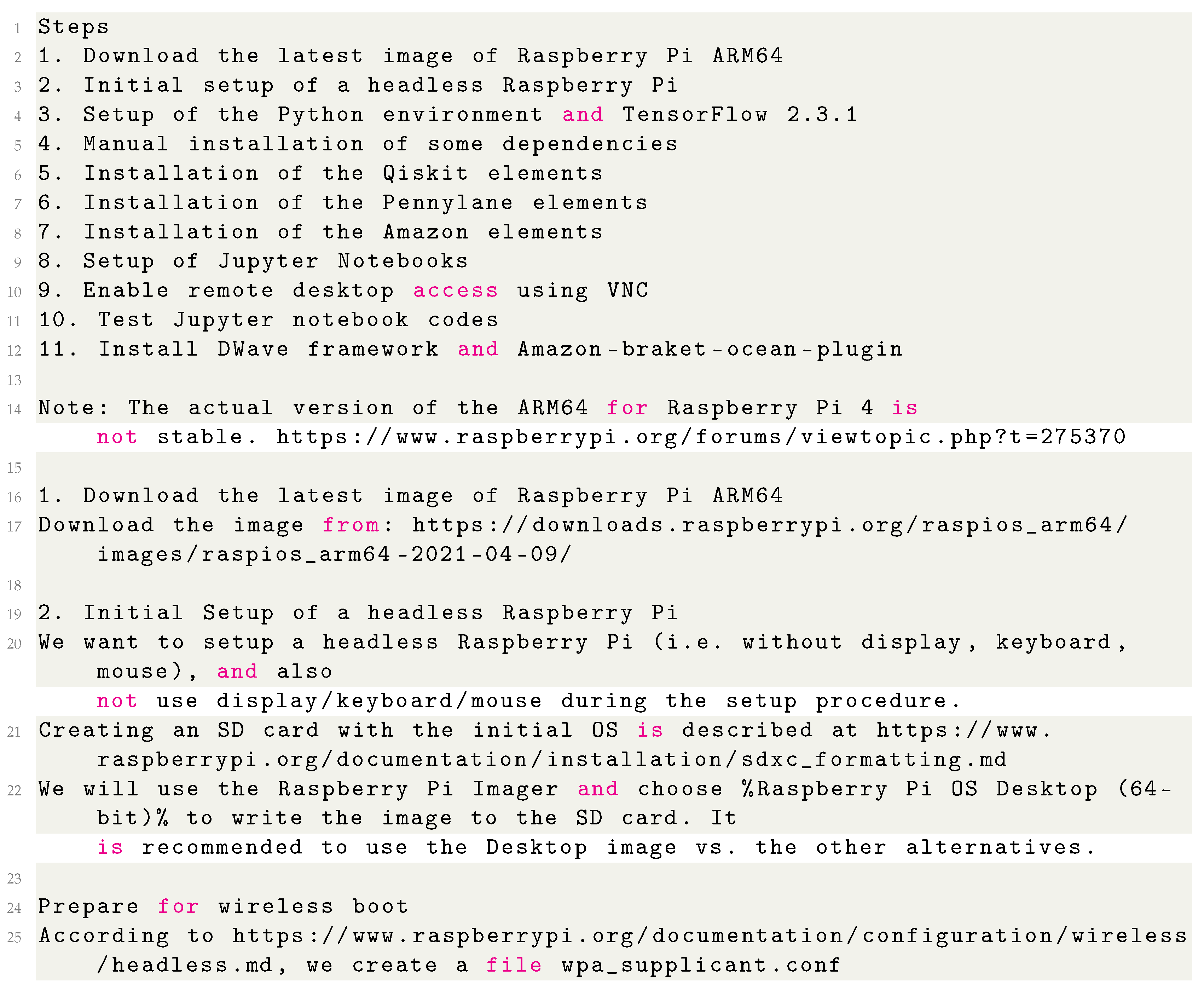
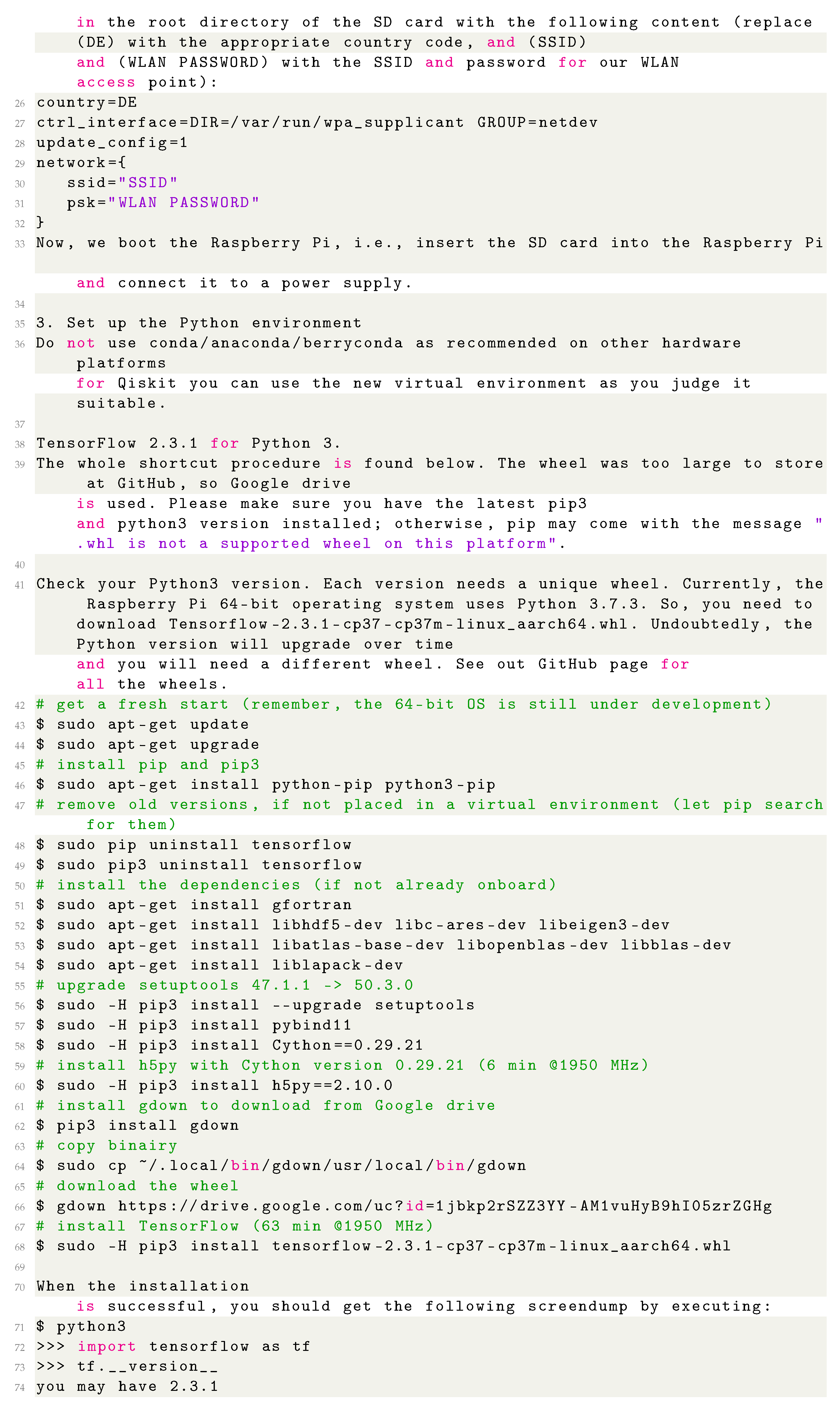
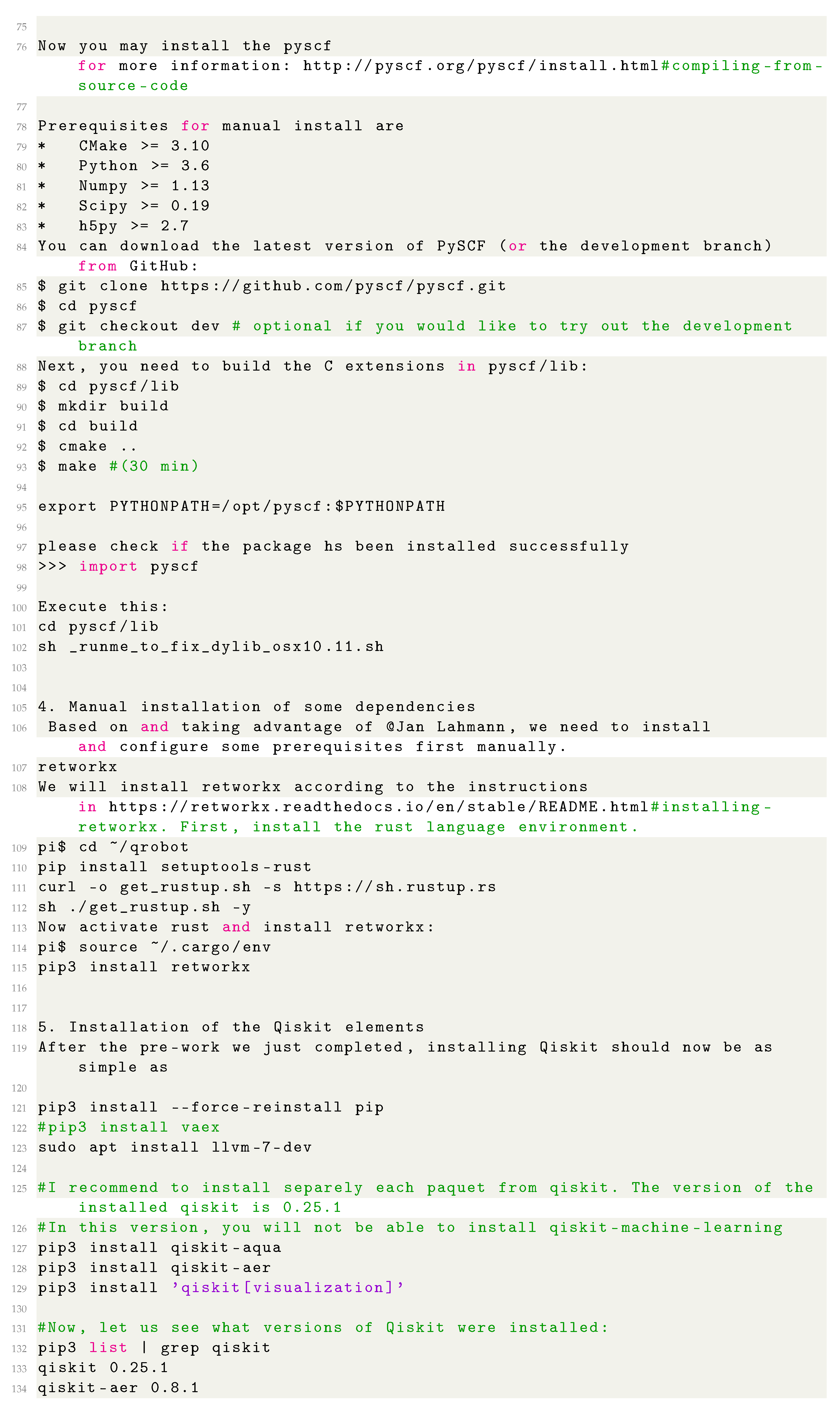
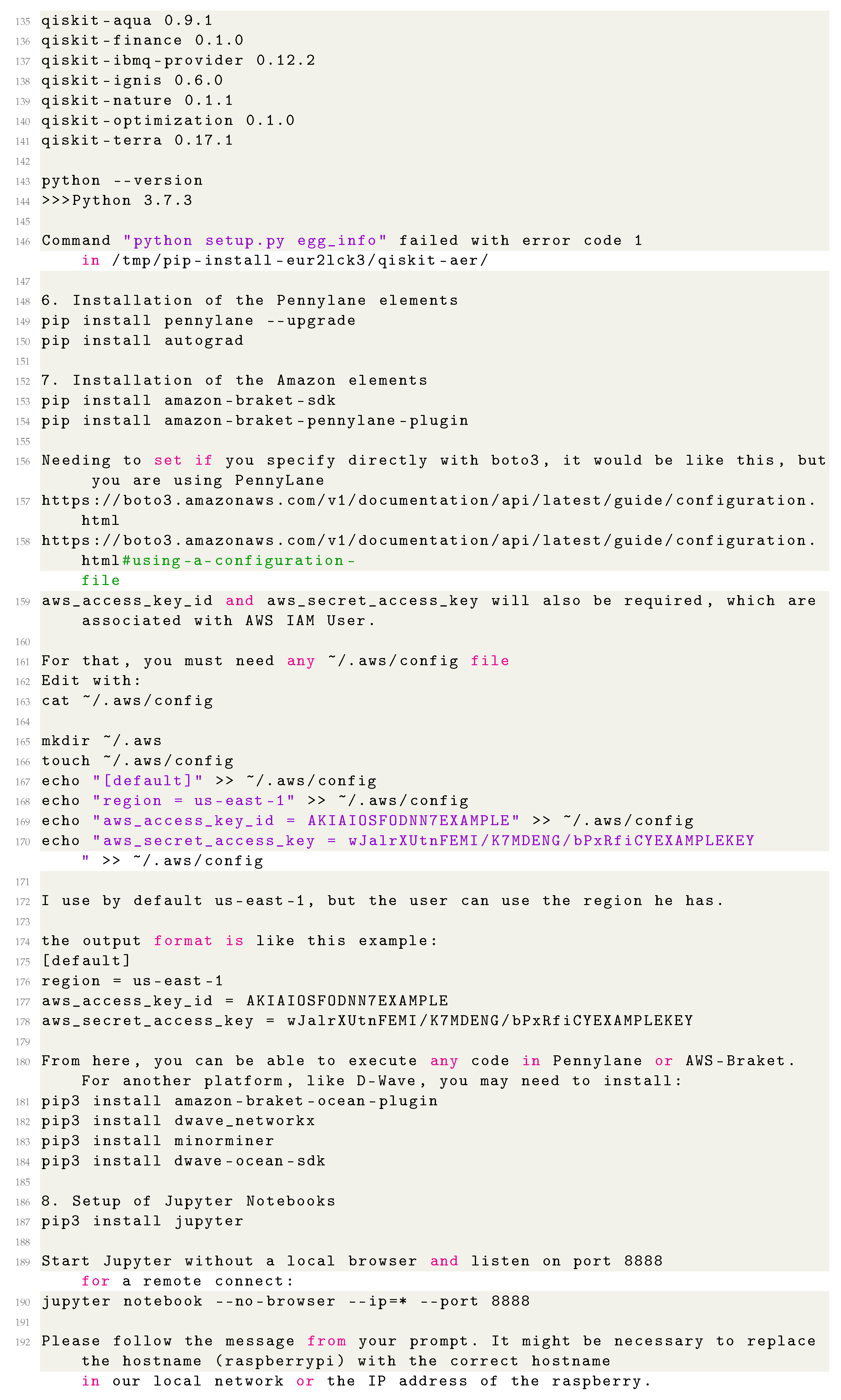
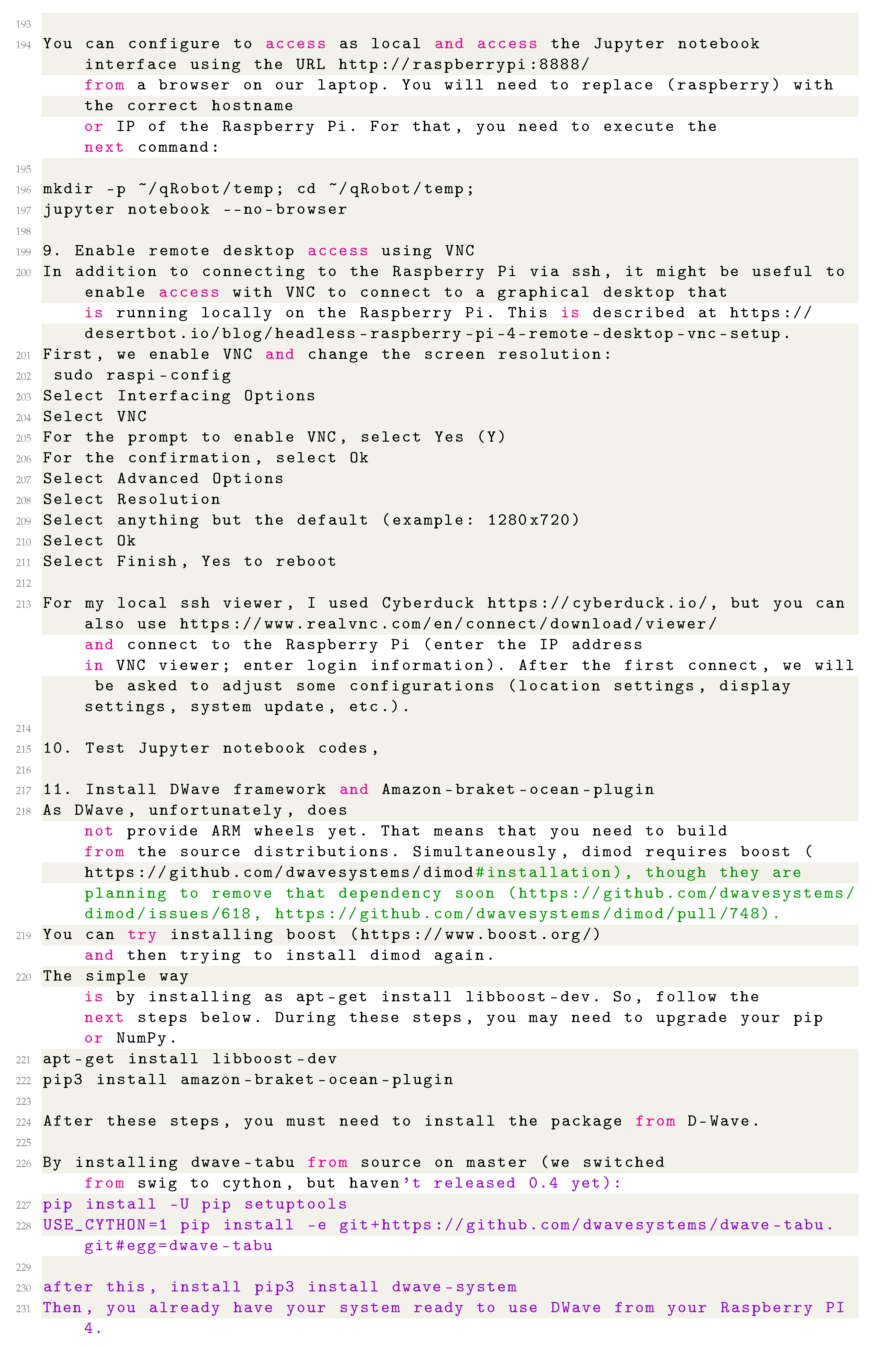
Appendix A. Installation of ARM64 on Raspberry Pi 4


References
- Angeleanu, A. New technology trends and their transformative impact on logistics and supply chain processes. Int. J. Econ. Pract. Theor. 2015, 5, 413–419. [Google Scholar]
- Kuźmicz, K.A. Benchmarking in omni-channel logistics. Res. Logist. Prod. 2015, 5, 491–501. [Google Scholar]
- Savelsbergh, M.; Van Woensel, T. 50th anniversary invited article—City logistics: Challenges and opportunities. Transp. Sci. 2016, 50, 579–590. [Google Scholar] [CrossRef]
- While, A.H.; Marvin, S.; Kovacic, M. Urban robotic experimentation: San Francisco, Tokyo and Dubai. Urban Stud. 2021, 58, 769–786. [Google Scholar] [CrossRef]
- Van der Aalst, W.M.; Bichler, M.; Heinzl, A. Robotic Process Automation; Springer: Cham, Switzerland, 2018. [Google Scholar]
- Siderska, J. Robotic Process Automation—A driver of digital transformation? Eng. Manag. Prod. Serv. 2020, 12, 21–31. [Google Scholar] [CrossRef]
- Agostinelli, S.; Marrella, A.; Mecella, M. Towards intelligent robotic process automation for BPMers. arXiv 2020, arXiv:2001.00804. [Google Scholar]
- Tompkins, J.A.; White, J.A.; Bozer, Y.A.; Tanchoco, J.M.A. Facilities Planning; John Wiley and Sons: Hoboken, NJ, USA, 2010. [Google Scholar]
- Karalekas, P.J.; Tezak, N.A.; Peterson, E.C.; Ryan, C.A.; da Silva, M.P.; Smith, R.S. A quantum-classical cloud platform optimized for variational hybrid algorithms. Quantum Sci. Technol. 2020, 5, 024003. [Google Scholar] [CrossRef] [Green Version]
- Cornet, B.; Fang, H.; Wang, H. Overview of Quantum Technologies, Standards, and their Applications in Mobile Devices. GetMobile Mob. Comput. Commun. 2021, 24, 5–9. [Google Scholar] [CrossRef]
- Chen, W.; Zheng, R.; Baade, P.D.; Zhang, S.; Zeng, H.; Bray, F.; Jemal, A.; Yu, X.Q.; He, J. Cancer statistics in China, 2015. CA Cancer J. Clin. 2016, 66, 115–132. [Google Scholar] [CrossRef] [Green Version]
- Bustillo-Lecompte, C.F.; Mehrvar, M. Slaughterhouse wastewater characteristics, treatment, and management in the meat processing industry: A review on trends and advances. J. Environ. Manag. 2015, 161, 287–302. [Google Scholar] [CrossRef]
- Koch, S.; Wäscher, G. A grouping genetic algorithm for the order batching problem in distribution warehouses. J. Bus. Econ. 2016, 86, 131–153. [Google Scholar] [CrossRef]
- Albareda-Sambola, M.; Fernández, E.; Hinojosa, Y.; Puerto, J. The multi-period incremental service facility location problem. Comput. Oper. Res. 2009, 36, 1356–1375. [Google Scholar] [CrossRef]
- Cergibozan, Ç.; Tasan, A.S. Order batching operations: An overview of classification, solution techniques, and future research. J. Intell. Manuf. 2019, 30, 335–349. [Google Scholar] [CrossRef]
- Azadnia, A.H.; Taheri, S.; Ghadimi, P.; Mat Saman, M.Z.; Wong, K.Y. Order batching in warehouses by minimizing total tardiness: A hybrid approach of weighted association rule mining and genetic algorithms. Sci. World J. 2013, 2013, 246578. [Google Scholar] [CrossRef]
- van Gils, T.; Katrien Ramaekers, A.C.; de Koster, R.B. Designing efficient order picking systems by combining planning problems: State-of-the-art classification and review. Eur. J. Oper. Res. 2018, 267, 1–15. [Google Scholar] [CrossRef] [Green Version]
- Duchoň, F.; Babinec, A.; Kajan, M.; Beňo, P.; Florek, M.; Fico, T.; Jurišica, L. Path planning with modified a star algorithm for a mobile robot. Procedia Eng. 2014, 96, 59–69. [Google Scholar] [CrossRef] [Green Version]
- LaValle, S.M.; Kuffner, J.J.; Donald, B. Rapidly-exploring random trees: Progress and prospects. Algorithmic Comput. Robot. New Dir. 2001, 5, 293–308. [Google Scholar]
- LaValle, S.M. Rapidly-Exploring Random Trees: A New Tool for Path Planning. 1998. Available online: https://www.cs.csustan.edu/~xliang/Courses/CS4710-21S/Papers/06%20RRT.pdf (accessed on 10 May 2021).
- Cheng, P.; LaValle, S.M. Resolution complete rapidly-exploring random trees. In Proceedings of the 2002 IEEE International Conference on Robotics and Automation, Washington, DC, USA, 11–15 May 2002; Volume 1, pp. 267–272. [Google Scholar]
- Rawlinson, N.; Sambridge, M. The fast marching method: An effective tool for tomographic imaging and tracking multiple phases in complex layered media. Explor. Geophys. 2005, 36, 341–350. [Google Scholar] [CrossRef] [Green Version]
- Gademann, N.; Van de velde, S. Order Batching to Minimize Total Travel Time in a parallel-aisle warehouse. IIE Trans. 2005, 37, 63–75. [Google Scholar] [CrossRef]
- Cortina, L.M.; Magley, V.J.; Williams, J.H.; Langhout, R.D. Incivility in the workplace: Incidence and impact. J. Occup. Health Psychol. 2001, 6, 64–80. [Google Scholar] [CrossRef]
- Hsu, C.M.; Chen, K.Y.; Chen, M.C. Batching orders in warehouses by minimizing travel distance with genetic algorithms. Comput. Ind. 2005, 56, 169–178. [Google Scholar] [CrossRef]
- Tsai, C.Y.; Liou, J.J.; Huang, T.M. Using a multiple-GA method to solve the batch picking problem: Considering travel distance and order due time. Int. J. Prod. Res. 2008, 46, 6533–6555. [Google Scholar] [CrossRef]
- Tsang, E. Foundations of Constraint Satisfaction: The Classic Text; BoD–Books on Demand: Norderstedt, Germany, 2014. [Google Scholar]
- Kochenberger, G.; Hao, J.K.; Glover, F.; Lewis, M.; Lü, Z.; Wang, H.; Wang, Y. The unconstrained binary quadratic programming problem: A survey. J. Comb. Optim. 2014, 28, 58–81. [Google Scholar] [CrossRef] [Green Version]
- Turing, A.M. On computable numbers, with an application to the Entscheidungsproblem. Proc. Lond. Math. Soc. 1937, 2, 230–265. [Google Scholar] [CrossRef]
- Feynman, R.P. Simulating physics with computers. Int. J. Theor. Phys 1982, 21, 467–488. [Google Scholar] [CrossRef]
- Deutsch, D. Quantum theory, the Church–Turing principle and the universal quantum computer. Proc. R. Soc. Lond. Math. Phys. Sci. 1985, 400, 97–117. [Google Scholar]
- Shor, P. Algorithms for quantum computation: Discrete logarithms and factoring. In Proceedings of the 35th Annual Symposium on Foundations of Computer Science, Santa Fe, NM, USA, 20–22 November 1994. [Google Scholar] [CrossRef]
- Grover, L.K. A fast quantum mechanical algorithm for database search. In Proceedings of the Twenty-Eighth Annual ACM Symposium on Theory of Computing—STOC ’96, New York, NY, USA, 22–24 May 1996. [Google Scholar] [CrossRef] [Green Version]
- Preskill, J. Quantum Computing in the NISQ era and beyond. Quantum 2018, 2, 79. [Google Scholar] [CrossRef]
- Wang, D.; Higgott, O.; Brierley, S. Accelerated Variational Quantum Eigensolver. Phys. Rev. Lett. 2019, 122. [Google Scholar] [CrossRef] [Green Version]
- Farhi, E.; Goldstone, J.; Gutmann, S. A Quantum Approximate Optimization Algorithm. arXiv 2014, arXiv:1411.4028. [Google Scholar]
- Schuld, M.; Sinayskiy, I.; Petruccione, F. An introduction to quantum machine learning. Contemp. Phys. 2014, 56, 172–185. [Google Scholar] [CrossRef] [Green Version]
- Biamonte, J.; Wittek, P.; Pancotti, N.; Rebentrost, P.; Wiebe, N.; Lloyd, S. Quantum machine learning. Nature 2017, 549, 195–202. [Google Scholar] [CrossRef]
- Pérez-Salinas, A.; Cervera-Lierta, A.; Gil-Fuster, E.; Latorre, J.I. Data re-uploading for a universal quantum classifier. Quantum 2020, 4, 226. [Google Scholar] [CrossRef]
- Atchade-Adelomou, P.; Golobardes-Ribe, E.; Vilasis-Cardona, X. Using the Parameterized Quantum Circuit combined with Variational-Quantum-Eigensolver (VQE) to create an Intelligent social workers’ schedule problem solver. arXiv 2020, arXiv:2010.05863. [Google Scholar]
- Atchade-Adelomou, P.; Casado-Fauli, D.; Golobardes-Ribe, E.; Vilasis-Cardona, X. quantum Case-Based Reasoning (qCBR). arXiv 2021, arXiv:cs.AI/2104.00409. [Google Scholar]
- Atchade-Adelomou, P.; Alonso-Linaje, G. Quantum Enhanced Filter: QFilter. arXiv 2021, arXiv:2104.03418. [Google Scholar]
- Kendon, V. Quantum computing using continuous-time evolution. Interface Focus 2020, 10, 20190143. [Google Scholar] [CrossRef]
- McGeoch, C.C. Adiabatic Quantum Computation and Quantum Annealing Theory and Practice. Synth. Lect. Quantum Comput. 2014, 5, 1–93. [Google Scholar] [CrossRef]
- McDonald, K.T. Ph410 Physics of Quantum Computation1. 2017. Available online: https://www.physics.princeton.edu/~mcdonald/examples/ph410problems.pdf (accessed on 10 May 2021).
- Landauer, E.O.W.R. Fundamental concepts of Hamiltonian Pauli Terms Quantum Computation. Available online: https://core.ac.uk/download/pdf/25212354.pdf (accessed on 10 May 2021).
- Harrow, A.W.; Farhi, E. Quantum Supremacy through the Quantum Approximate Optimization Algorithm. 2019. Available online: https://arxiv.org/pdf/1602.07674.pdf (accessed on 10 May 2021).
- Kadowaki, T.; Nishimori, H. Quantum Annealing in the Transverse Ising Model. Phys. Rev. E 1998, 58, 5355. [Google Scholar] [CrossRef] [Green Version]
- Laporte, G. The Vehicle Routing Problem: An Overview of Exact and Approximate Algorithm. Eur. J. Oper. Res. 1992, 59, 345–358. [Google Scholar] [CrossRef]
- Sarkar, K.B.A.; Mouedenne, A.; Hubregtsen, A.Y.T.; Krol, I.A.A. Quantum Computer Architecture: Towards Full-Stack Quantum Accelerators. In Proceedings of the Design, Automation & Test in Europe Conference & Exhibition (DATE), Grenoble, France, 9–13 March 2020. [Google Scholar]
- Ross, B.O.B.J.; Hanshar, F. Multi-objective Genetic Algorithms for Vehicle Routing Problem with Time Windows. Appl. Intell. 2004, 24, 17–30. [Google Scholar]
- Peruzzo, A.; McClean, J.; Shadbolt, P.; Yung, M.H.; Zhou, X.Q.; Love, P.J.; Aspuru-Guzik, A.; O’Brien, J.L. A variational eigenvalue solver on a photonic quantum processor. Nat. Commun. 2014, 5. [Google Scholar] [CrossRef] [Green Version]
- Matsuura, G.G.G.A.Y. QAOA for Max-Cut Requires Hundreds of Qubits for Quantum Speed-up. Sci. Rep. 2019, 9, 1–7. [Google Scholar]
- Moor, J.D.B.D. The Clifford Group, Stabilizer States, and Linear and Quadratic Operations over GF(2). Phys. Rev. A 2003, 68, 042318. [Google Scholar]
- Rebentrost, P.; Schuld, M.; Wossnig, L.; Petruccione, F.; Lloyd, S. Quantum gradient descent and Newton’s method for constrained polynomial optimization. arXiv 2018, arXiv:quant-ph/1612.01789. [Google Scholar] [CrossRef]
- Vyskocil, T.; Djidjev, H. Embedding Equality Constraints of Optimization Problems into a Quantum Annealer. Algorithms 2019, 12, 77. [Google Scholar] [CrossRef] [Green Version]
- Anuradha Mahasinghe Michael, J.; Dinneen, R.H. Solving the Hamiltonian Cycle Problem using a Quantum Computer. In Proceedings of the Australasian Computer Science Week Multiconference, Sydney, NSW, Australia, 29–31 January 2019. [Google Scholar]
- Lucas, A. Ising formulations of many NP problems. Front. Phys. 2014, 2, 5. [Google Scholar] [CrossRef] [Green Version]
- Roch, S.F.C.; Gabor, T.; Seidel, C.; Neukart, F.; Galter, I.; Mauerer, W.; Linhoff-Popien, C. A Hybrid Solution Method for the Capacitated Vehicle Routing Problem Using a Quantum Annealer. Front. ICT 2019, 6, 13. [Google Scholar]
- Braket, A. Amazon Braket Services. 2021. Available online: https://aws.amazon.com/braket/?nc1=h_ls (accessed on 5 May 2021).
- Xie, L.; Li, H.; Luttmann, L. Formulating and solving integrated order batching and routing in multi-depot AGV-assisted mixed-shelves warehouses. arXiv 2021, arXiv:math.OC/2101.11473. [Google Scholar]
- Arutyunov, G.; Frolov, S.; Staudacher, M. Bethe Ansatz for Quantum Strings. J. High Energy Phys. 2004, 2004, 16. [Google Scholar] [CrossRef] [Green Version]
- Sim, S.; Johnson, P.D.; Aspuru-Guzik, A. Expressibility and Entangling Capability of Parameterized Quantum Circuits for Hybrid Quantum-Classical Algorithms. Adv. Quantum Technol. 2019, 2, 1900070. [Google Scholar] [CrossRef] [Green Version]
- Atchade-Adelomou, P.; Golobardes-Ribé, E.; Vilasís-cardona, X. Using the Variational-Quantum-Eigensolver (VQE) to Create an Intelligent Social Workers Schedule Problem Solver. In Proceedings of the International Conference on Hybrid Artificial Intelligence Systems, Gijón, Spain, 11–13 November 2020; pp. 245–260. [Google Scholar]
- Wu, C.W. On Rayleigh–Ritz ratios of a generalized Laplacian matrix of directed graphs. Linear Algebra Its Appl. 2005, 402, 207–227. [Google Scholar] [CrossRef] [Green Version]
- Foundation, R.P. Raspberry Pi 4. 2021. Available online: https://www.raspberrypi.org/products/raspberry-pi-4-model-b/ (accessed on 10 May 2021).
- Jaggar, D. ARM architecture and systems. IEEE Ann. Hist. Comput. 1997, 17, 9–11. [Google Scholar] [CrossRef]
- Jiang, Q.; Lee, Y.C.; Zomaya, A.Y. The Power of ARM64 in Public Clouds. In Proceedings of the 2020 20th IEEE/ACM International Symposium on Cluster, Cloud and Internet Computing (CCGRID), Melbourne, Australia, 11–14 May 2020; pp. 459–468. [Google Scholar]
- Wille, R.; Van Meter, R.; Naveh, Y. IBM’s Qiskit Tool Chain: Working with and Developing for Real Quantum Computers. In Proceedings of the 2019 Design, Automation & Test in Europe Conference & Exhibition (DATE), Florence, Italy, 25–29 March 2019; pp. 1234–1240. [Google Scholar]
- IBM. DOcplex Python Modeling API. 2021. Available online: https://www.ibm.com/docs/en/icos/12.9.0?topic=docplex-python-modeling-api (accessed on 10 May 2021).
- Eisberg, R.; Resnick, R. Quantum Physics of Atoms, Molecules, Solids, Nuclei, and Particles. 1985. Available online: https://ui.adsabs.harvard.edu/abs/1985qpam.book.....E/abstract (accessed on 10 May 2021).
- Iterate. Cyberduck—SSH. 2021. Available online: https://cyberduck.io/sftp/ (accessed on 10 May 2021).
- The Raspberry Pi Foundation. Configuration of the Raspberry Pi. 2021. Available online: https://www.raspberrypi.org/documentation/configuration/ (accessed on 10 May 2021).
- Bergholm, V.; Izaac, J.; Schuld, M.; Gogolin, C.; Alam, M.S.; Ahmed, S.; Arrazola, J.M.; Blank, C.; Delgado, A.; Jahangiri, S.; et al. PennyLane: Automatic Differentiation of Hybrid Quantum-Classical Computations. arXiv 2020, arXiv:quant-ph/1811.04968. [Google Scholar]
- Braket, A. Github Amazon Braket. 2021. Available online: https://github.com/aws/amazon-braket-sdk-python (accessed on 26 February 2021).
- Sete, E.A.; Zeng, W.J.; Rigetti, C.T. A functional architecture for scalable quantum computing. In Proceedings of the 2016 IEEE International Conference on Rebooting Computing (ICRC), San Diego, CA, USA, 17–19 October 2016; pp. 1–6. [Google Scholar]
- McKay, D.C.; Alexander, T.; Bello, L.; Biercuk, M.J.; Bishop, L.; Chen, J.; Chow, J.M.; Córcoles, A.D.; Egger, D.; Filipp, S.; et al. Qiskit backend specifications for openqasm and openpulse experiments. arXiv 2018, arXiv:1809.03452. [Google Scholar]
- D-Wave. D-Wave Computer. 2021. Available online: https://www.dwavesys.com/quantum-computing (accessed on 10 May 2021).
- PennyLane, A.B. PennyLane-Braket Plugin. 2021. Available online: https://amazon-braket-pennylane-plugin-python.readthedocs.io/en/latest/ (accessed on 26 February 2021).
- PennyLane, A.B. PennyLane-Braket Plugin. 2021. Available online: https://docs.aws.amazon.com/braket/latest/developerguide/braket-devices.html (accessed on 26 March 2021).
- Zaborniak, T.; de Sousa, R. Benchmarking Hamiltonian Noise in the D-Wave Quantum Annealer. IEEE Trans. Quantum Eng. 2021, 2, 1–6. [Google Scholar] [CrossRef]
- Atchade-Adelomou, P.; Golobardes-Ribé, E.; Vilasis-Cardona, X. Formulation of the Social Workers’ Problem in Quadratic Unconstrained Binary Optimization Form and Solve It on a Quantum Computer. J. Comput. Commun. 2020, 8, 44–68. [Google Scholar] [CrossRef]
- Braket, A. qRobot Platform. 2021. Available online: https://github.com/pifparfait/qRobot_Platform/blob/main/RaspberryPi_ARM64_for_QML.ipynb (accessed on 26 June 2021).


| The Benchmark of the qRobot’s Algorithm in Different Quantum Simulators. | ||||
|---|---|---|---|---|
| # of Items | # Qubits | DWave—Time (s) | Ibmq_qasm_simulator—Time (s) | Pennylane—Time (s) |
| 2 | 18 | 1.92 | 1.89 | 1.94 |
| 3 | 26 | 3.2 | 737.46 | 656.93 |
| 4 | 36 | 4.88 | - | - |
| 5 | 48 | 7.60 | - | - |
| 6 | 62 | 11.16 | - | - |
| 7 | 78 | 15.89 | - | - |
| 8 | 96 | 21.72 | - | - |
| 9 | 116 | 30.18 | - | - |
| 10 | 138 | 43.29 | - | - |
| 11 | 162 | 53.28 | - | - |
| 12 | 188 | 63.45 | - | - |
| AWS-Braket [75] | ibmq_qasm_simulator [69] | Pennylane [74] | |||
|---|---|---|---|---|---|
| # of Items | qRobot’s Capacity | # Qubits | Average Time (s) | Average Time (s) | Average Time (s) |
| 2 | 15 | 10 | |||
| 3 | 15 | 16 | |||
| 4 | 15 | 24 | 480 | ||
| 5 | 15 | 34 | − | − | |
| 6 | 15 | 46 | − | − | |
| 7 | 15 | 60 | − | − | |
| 8 | 15 | 76 | − | − | |
| 9 | 15 | 94 | − | − | |
| 10 | 25 | 115 | − | − | |
| 11 | 25 | 137 | − | − | |
| 12 | 25 | 161 | − | − |
Publisher’s Note: MDPI stays neutral with regard to jurisdictional claims in published maps and institutional affiliations. |
© 2021 by the authors. Licensee MDPI, Basel, Switzerland. This article is an open access article distributed under the terms and conditions of the Creative Commons Attribution (CC BY) license (https://creativecommons.org/licenses/by/4.0/).
Share and Cite
Atchade-Adelomou, P.; Alonso-Linaje, G.; Albo-Canals, J.; Casado-Fauli, D. qRobot: A Quantum Computing Approach in Mobile Robot Order Picking and Batching Problem Solver Optimization. Algorithms 2021, 14, 194. https://0-doi-org.brum.beds.ac.uk/10.3390/a14070194
Atchade-Adelomou P, Alonso-Linaje G, Albo-Canals J, Casado-Fauli D. qRobot: A Quantum Computing Approach in Mobile Robot Order Picking and Batching Problem Solver Optimization. Algorithms. 2021; 14(7):194. https://0-doi-org.brum.beds.ac.uk/10.3390/a14070194
Chicago/Turabian StyleAtchade-Adelomou, Parfait, Guillermo Alonso-Linaje, Jordi Albo-Canals, and Daniel Casado-Fauli. 2021. "qRobot: A Quantum Computing Approach in Mobile Robot Order Picking and Batching Problem Solver Optimization" Algorithms 14, no. 7: 194. https://0-doi-org.brum.beds.ac.uk/10.3390/a14070194