
Self-Adaptive Path Tracking Control for Mobile Robots under Slippage Conditions Based on an RBF Neural Network

School of Mechanical Engineering, University of Science and Technology Beijing, Beijing 100083, China
*
Author to whom correspondence should be addressed.
Algorithms 2021, 14(7), 196; https://0-doi-org.brum.beds.ac.uk/10.3390/a14070196
Submission received: 3 June 2021
/
Revised: 24 June 2021
/
Accepted: 27 June 2021
/
Published: 28 June 2021
Abstract
:Wheeled mobile robots are widely implemented in the field environment where slipping and skidding may often occur. This paper presents a self-adaptive path tracking control framework based on a radial basis function (RBF) neural network to overcome slippage disturbances. Both kinematic and dynamic models of a wheeled robot with skid-steer characteristics are established with position, orientation, and equivalent tracking error definitions. A dual-loop control framework is proposed, and kinematic and dynamic models are integrated in the inner and outer loops, respectively. An RBF neutral network is employed for yaw rate control to realize adaptability to longitudinal slippage. Simulations employing the proposed control framework are performed to track snaking and a DLC reference path with slip ratio variations. The results suggest that the proposed control framework yields much lower position and orientation errors compared with those of a PID and a single neuron network (SNN) controller. It also exhibits prior anti-disturbance performance and adaptability to longitudinal slippage. The proposed control framework could thus be employed for autonomous mobile robots working on complex terrain.
1. Introduction
Path tracking is critical for autonomous driving, as it moves a mobile robot to follow a desired path by longitudinal and lateral control [1]. The linear quadratic regulator (LQR) controller, proportional–integrated–derivative (PID) controller, and sliding mode controller are often used in path tracking control [2,3,4]. In addition, model predictive control (MPC) is often used in path tracking. Model predictive control strategies are applied to a wheeled mobile robot, and it has proved that MPC reduces energy consumption by 70% compared to the reduction in energy consumption provided by PID control [5]. The various path tracking control algorithms proposed for mobile robots usually employ constant control parameters, which yield optimal performance under a no-disturbance condition. Researchers focused on selecting suitable controller gains and designing compensators to improve control performance [6,7,8]. Adaptive control methods were widely utilized for systems with unknown dynamics and uncertain disturbances [9,10]. The terrain changes, often considered disturbances for controller design, may have a variety of effects on a robot’s motion, such as slipping and skidding [11,12]. Slippage, however, is especially crucial for the motion control of mobile robots working in the field environment [13]. Such disturbances may lead to the degradation of tracking performance [14].
A number of studies in the literature took slippage into account and proposed path tracking control together with slipping and skidding compensation [15]. Therefore, the accuracy of slippage parameter estimation is vital to the design of such controllers. The generalized extended state observer (GESO) approach and Kalman filter were utilized to estimate the slipping parameter of wheels [13,16], and the slippage effect was considered in a kinematic model to improve the performance of path tracking [17,18,19]. The disturbance led by slipping and skidding, however, is difficult to estimate and predict. Only few studies have presented adaptive controllers with time-varying parameters to adapt to various terrains. An improved adaptive controller was proposed to allow a wheeled mobile robot (WMR) to track the desired trajectory under unknown longitudinal slip [14]. The accuracy and reliability of the path tracking of a four-wheel mobile robot when moving at high dynamics on a slippery surface were addressed by employing an adaptive and predictive controller [20]. A novel indirect adaptive controller was proposed to allow wheeled robots to finish path tracking on complicated terrains in the presence of unknown interferences and wheel slippage using integral sliding mode control (ISMC)-based neural networks with updated rules for adjustments the weights [21]. A self-tuning methodology based on probabilistic approaches and machine learning techniques was proposed to improve the path tracking performance of for autonomous vehicles maneuvering along changing terrain [22]. A new adaptive control scheme was used to overcome the difficulties in path tracking, and the scheme included designing a new adaptive state-feedback controller and two high-gain observers to estimate the unknown linear and angular velocities, respectively [23]. The adaptive sliding mode control (SMC) method combines the adaptive control method and a fast double power reaching law with the SMC method, and a complete control loop with active slip compensation and adaptive SMC is thus established [24]. The path tracking controller for field robots should overcome the terrain changes by employing a time-varying controller that can adapt to slippage disturbances.
This paper addresses the problem of degradation on path tracking performance in WMRs due to slipping and skidding for. The major contributions of this paper are listed as follows:
- An equivalent error integrating position and orientation errors, and taking account of the preview distance is employed for the development of path tracking control to achieve both a lower position error and a steady posture.
- A dual-loop control framework that integrates kinematic and dynamic models in the inner and outer loops, respectively, is proposed. A decoupled control method including a yaw rate controller and a speed controller is utilized to achieve the tracking target of a reference path with a desired speed.
- An RBF neural network is employed for yaw rate control to realize adaptability to longitudinal slipping and skidding caused by complex terrain.
The remainder of this paper is organized as follows: In Section 2, a kinematic model of a skid–steer wheeled robot is formulated with the definition of position and orientation errors. Dynamic equations for the robot are also derived for path tracking controller design. Section 3 introduces the dual-loop control framework for path tracking. Section 4 describes simulation results by tracking a snaking and a DLC reference path under variations in slip ratios. Finally, the conclusion and future work of this paper are shown in Section 5.
2. Kinematic and Dynamic Models
Kinematic and dynamic models are widely used to estimate robot behaviors and dynamic response under the control input, which is essential for the development of a controller. Both kinematic and dynamic models of a WMR with skid–steer characteristics are established. Path tracking errors defined by driver-preview theory are included in the kinematic model. Dynamic equations for the wheeled robot are formulated and used for the inner-loop control of the proposed framework.
2.1. Kinematic Model
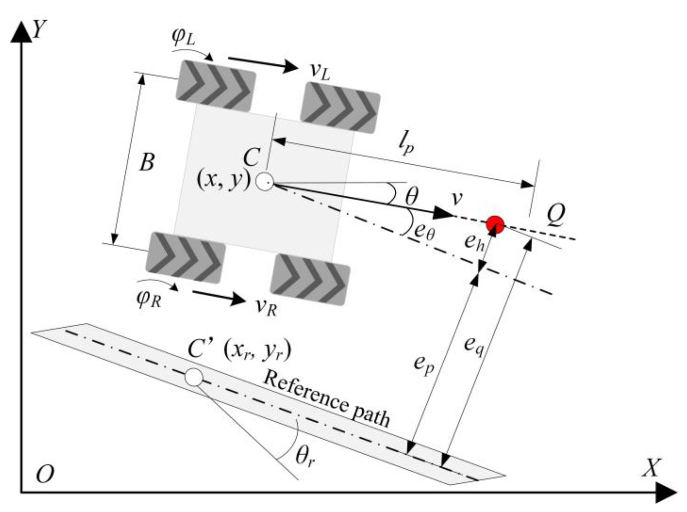
A kinematic model is firstly established for a skid–steer WMR to acquire its trajectory and orientation variation under tracking control. Figure 1 shows a description of the kinematic model with the error definition for path tracking. The position and orientation of the wheeled robot can be explained with the world coordinate system . is the center of gravity (CG) of the robot, which is taken as the reference point of path tracking in this study. The wheeled robot consists of two driving rear wheels and two driven front wheels, and steering is achieved by the speed difference between the two rear wheels.
A generalized coordinate vector of the wheeled robot is defined, where and denote the coordinates along the X and Y orientations of CG of the robot: is the orientation angle of the robot with respect to the x-axis; and and are the rotation angles of the left and right driving wheels, respectively. The kinematic equation of a skid–steer wheeled robot is described as
where and are formulated as
where is the radius of a driving wheel, and is the distance between the centerlines of left and right wheels.
The non-holonomic constraint that a wheeled robot is subjected to is given by
where is
The non-holonomic constraint is under the assumption that the system is “pure rolling without slipping” [25]. Wheeled robots working in a field environment often slip or skid, and thus, the kinematic equation is rewritten by taking the slip ratio into account. The kinematic model of a skid–steer wheeled robot under slippage conditions could be obtained as
where and are the slip ratios of left and right wheels, respectively, which are defined as
where and are the linear velocities of the left and right wheels, respectively.
Path tracking errors of the robot are composed of position errors in both the lateral and longitudinal directions, as well as orientations with respect to the reference path, which are defined as
where and are the position and orientation errors, respectively, of the robot with respect to the reference path; represents the reference position; is the reference orientation. is equal to 1 when the robot is at the left side of the reference path, while is −1 when it is at the right side.
In this paper, an equivalent tracking error is defined by taking the preview distance into account, which represents a position error of a future state [26]:
where is a position error in the future, which is caused by the orientation error of the current state. All of the defined errors are employed as the input and evaluation indicators for controller development.
2.2. Dynamic Model
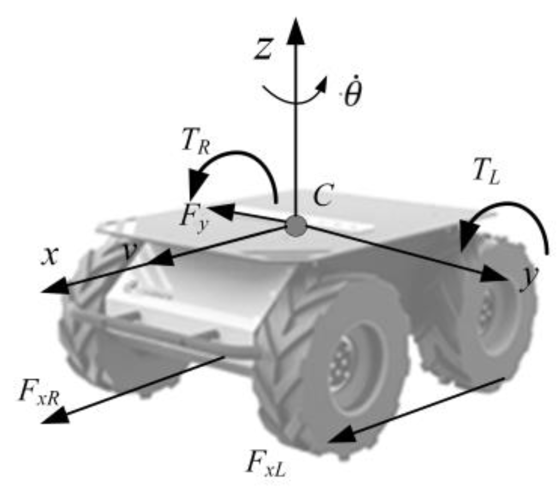
A dynamic model is subsequently built for the wheeled robot to take dynamic constraints of the motor driving system into account. The dynamic model, as shown in Figure 2, can be explained with a body-fixed coordinate system, where the origin point is located at the CG of the robot. and are driving torques on wheels generated by left and right motors, respectively. denotes constraint force along the y-axis, while and are constraint forces on the left and right wheels along the x-axis.
In this paper, it is assumed that the robot is constrained to moving on the horizontal plane only. The dynamic equation of the system is formulated using the Lagrange method, which can be expressed as
where is the inertial matrix, is the transfer matrix, denotes the input vector of driving torques, and is the vector of constraint forces.
where m is the mass of the robot, J is its moment of inertia along the z-axis, and are the moments of inertia of the left and right driving wheels, respectively.
The vector of constraint forces can be defined as follows
where and represent the longitudinal stiffness of the left and right driving wheels, respectively; is the cornering stiffness of the wheels; is the wheel slip angle.
The wheel slip angle can be estimated by the velocity variables of the previous time, and can be expressed as follows
where is the value of at t moment; is the value of at t − 1 moment; and are the values of and , respectively, at t − 1 moment.
The dynamic equation (Equation (10)) can thus be simplified as
The angular acceleration of the left and right driving wheels can be obtained, and it is employed to design the inner loop of the control framework in this paper.
3. Path Tracking Controller
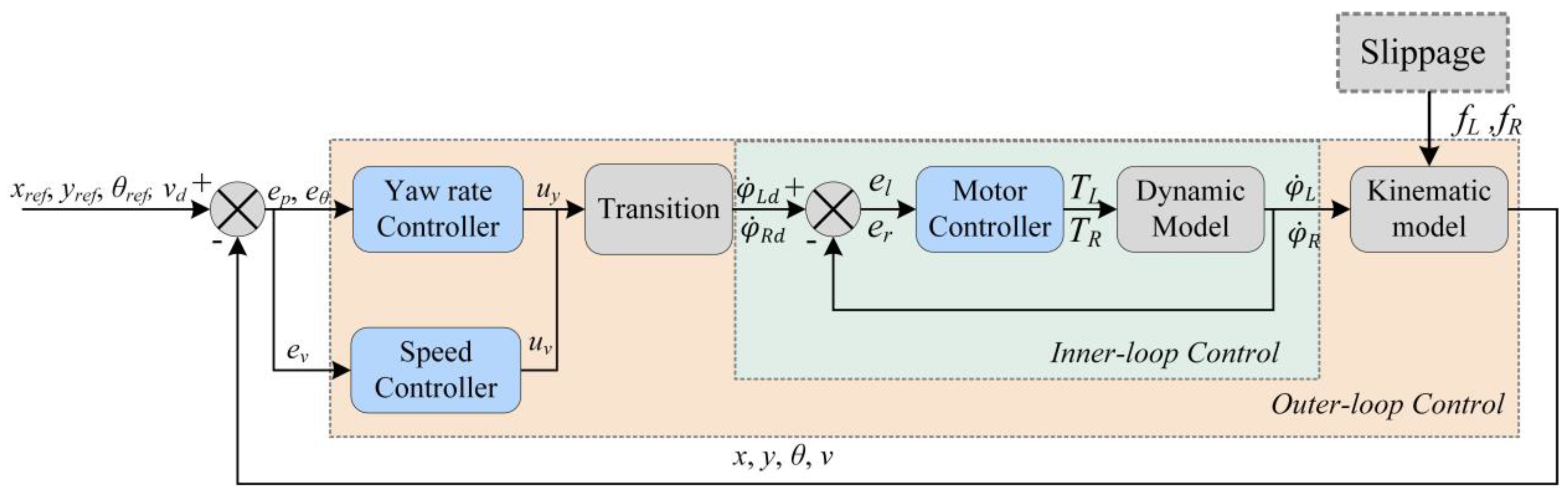
Figure 3 shows the configuration of the proposed dual-loop control framework for path tracking. A decoupled control method, including a yaw rate controller and a speed controller, is employed to achieve the tracking target of a given path with a desired speed, which is defined as . The yaw rate controller is developed to move the robot following the reference path. Slipping and skidding may lead to degradation of the path tracking performance of a conventional controller. An RBF neural network is thus utilized to propose a self-adaptive tracking control due to its prior adaptability to various systems and performance against disturbances. At the same time, a speed controller is designed to compensate the loss of robot speed due to the occurrence of slipping and skidding. A motor controller is also developed to achieve the reference angular velocity of the left and right driving wheels. Both dynamic and a kinematic controls are realized in the inner and outer loops of the proposed control framework. Slipping and skidding are simulated as unexpected disturbances of the kinematic model, and the adaptive performance of the proposed framework is investigated.
According to the configuration of the path tracking control framework from Figure 3, the real path can be output in Algorithm 1.
| Algorithm 1 Self-adaptive path tracking control algorithm based on RBF neural network | ||
| Input: p = {, , , }; | ||
| Output: O = {x, , , }; | ||
| 1: | while t < tmax | |
| 2: | //outer-loop control algorithm | |
| 3: | (t) ← Error((t), (t), (t), (t)); | //Compute error |
| 4: | [(t); (t)] ← Error([(t), (t)]; [(t), (t)]); | |
| 5: | (t) ← Speedcontroller((t)); | //PID control algorithm (Equation (15)) |
| 6: | The yaw rate controller input x(t) = {(t), (t), (t), (t)}; | |
| 7: | if t = 0 then | |
| 8: | Initialize matrix w(t), b(t) and c(t); | |
| 9: | else | |
| 10: | h(t) ← Hiddenlayer(x(t), b(t), c(t)); | //Compute hidden layer output matrix (Equation (18)) |
| 11: | (t) ← RBFoutput(w(t), h(t)); | //Equation (19) |
| 12: | Update matrix w(t + 1), b(t + 1) and c(t + 1); | //Equations (21) and (23) |
| 13: | end if | |
| 14: | [(t), (t)] ← Transition((t), (t)); | //The desired angular velocity |
| 15: | //Inner-loop control algorithm | |
| 16: | [(t); (t)] ← Error([(t), (t)]; [(t), (t)]); | |
| 17: | [(t); (t)] ← Motorcontroller([(t); (t)]); | //PID control algorithm (Equation (16)) |
| 18: | [(t + 1); (t + 1)] ← Dynamicmodel([(t); (t)]), and feedback to step 16 of the t + 1 moment; | |
| 19: | //Inner-loop control closure | |
| 20: | O(t + 1) ← Kinematicmodel((t + 1), (t + 1), (t + 1), (t + 1)), and feedback to step 3–4 of the t + 1 moment; | |
| 21: | t ← t + 1; | |
| 22: | //Outer-loop control closure | |
| 23: | end while | |
| 24: | returnO; | |
3.1. Speed and Motor Control
Both and the speed controller output are the inputs of robot model through angular velocity transition. The PID control algorithm is employed to develop the speed controller and motor controller, which are shown in Figure 3. The speed controller is designed as
where , , and are the proportional, integral, and differential coefficients of the speed controller, respectively, and is the difference between the desired velocity and actual velocity of the robot.
The PID control algorithm of the motor controller is derived as
where , , and are the proportional, integral, and differential coefficients of the motor controller, respectively; is the torque output by the PID control algorithm; is the difference between the desired angular velocity and the actual angular velocity of the s-wheel. and represent left and right sides of the robot, respectively.
The motor controller uses the DC motor, and the DC motor is derived as
where is the actual torque output by the DC motor, is torque constant of the motor, and is the motor current. In motor control, the influence of damping torque must not be ignored. Therefore, the damping term is considered in the motor control, and is the damping coefficient [5].
In the PID control algorithm, it is difficult to obtain reasonable proportional, integral, and differential coefficients. In this paper, the following steps are used to tune the PID controller, and the corresponding coefficient is obtained:
- Firstly, the proportional coefficient is tuned. The initial value can be calculated quantitatively, and the different values from both sides of the initial value can be taken. The final proportional coefficient can be determined when the system has a relatively fast response speed.
- Secondly, the integral coefficient is tuned. The time for the system to reach stability is tested when the value is 0–1, and the integral coefficient can be determined when the time is relatively short.
- Thirdly, the differential coefficient is tuned. The differential coefficient, which is 0–1, can be determined when the system is relatively stable.
According to the above method of tuning the PID controller, the coefficients of the speed controller , , and are 50, 0.5, and 0, respectively, and the coefficients of the motor controller , , and are 4, 0, and 1, respectively.
3.2. Yaw Rate Control
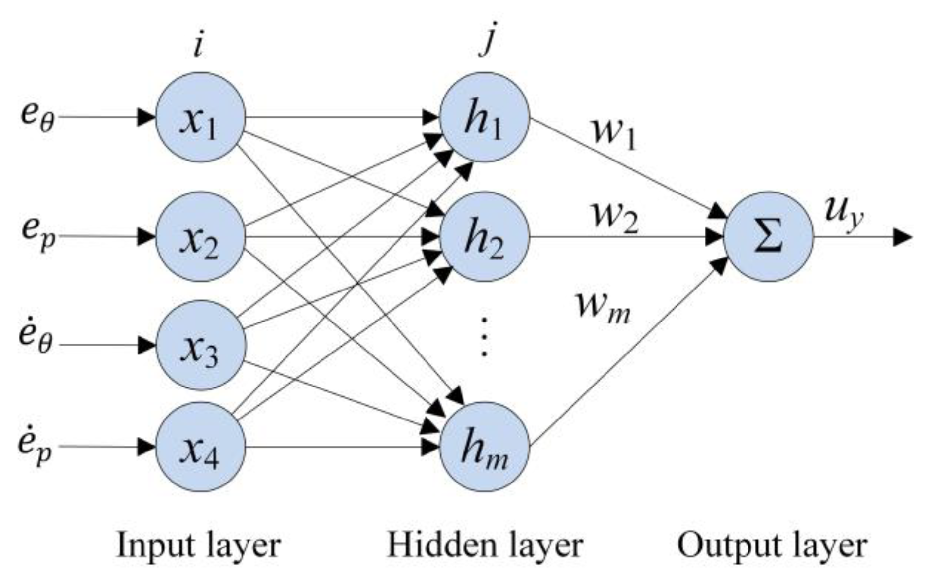
The yaw rate controller, as shown in Figure 4, is developed from an RBF neural network where an online adaptive law is applied. The neural network is composed of an input layer, a hidden layer, and an output layer. Position and orientation errors, as well as their deviations, are taken as the input of the neural network. The output is the desired yaw rate of the wheeled robot, which is denoted as uy. In this paper, a 4–9–1 structure is employed to facilitate the RBF neural network, and a self-adaptive law is applied to update the network parameters online.
As shown in Figure 4, is defined as the network input, and is the output of hidden layer, where represents the value of the Gaussian function for the jth neuron.
where is the central vector, is the width vector of the Gaussian function, and , is the number of neurons in the hidden layer.
The output of the neural network is
where is the weight of output layer from the jth neuron.
An error indicator of the network is defined as
In this paper, is defined as a weighted error with the equivalent tracking error and its deviation
where and are the weight coefficients of and , respectively.
The changes in the weight are , , and , and they are derived using the gradient descent method to update the network.
where η is the learning rate, and the value is between 0 and 1.
When the value of η is too low, the speed of learning decreases. On the contrary, when the value of η is too high, the change in the weight is unstable. Therefore, the momentum term is added to Equation (22). If the gradient direction of the current time is similar to that of the historical time, the gradient direction of the current time is strengthened; if it is different, the gradient direction at the current time weakens. The weight of the output layer, the width, and center vectors of the Gaussian function can be updated by
where α is factor of momentum, and the value is between 0 and 1.
A PID tracking controller is also formulated for the wheeled robot to obtain the central vector values of the RBF network. Path tracking simulations are conducted by employing the PID controller, and both position error and orientation error are collected to determine the central vector of the RBF network by the K-means clustering method. In the simulation employing the PID controller, the slippage disturbances are not taken into account. The purpose of such simulation is to identify a suitable central vector for the RBF network rather than a random approach.
4. Results and Discussion
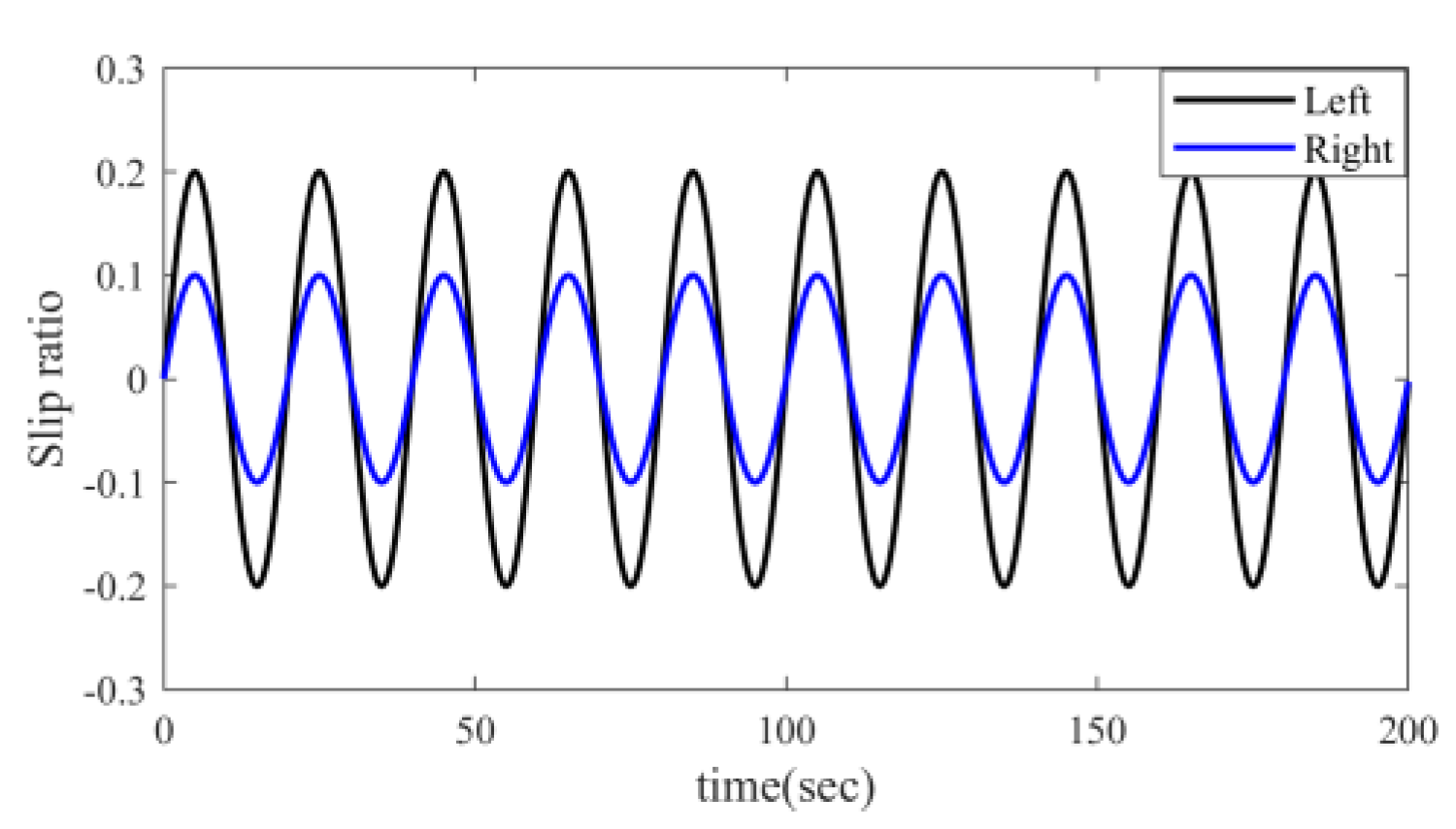
The proposed path tracking algorithm is verified by tracking two different reference paths, namely, a snaking path and a double lane change (DLC) path. As shown in Figure 5, the robot tracks the path on a separation surface, and the slip ratios of the left and right wheels are taken as disturbances input to the kinematic model. The effectiveness and adaptability of the proposed control framework are demonstrated under tracking simulations.
4.1. Algorithm Verification
The parameters of the wheeled robot for algorithm verification are listed in Table 1. The learning rate η and factor of momentum α in the RBF network are set to 0.3 and 0.35, respectively. The weight coefficients and are 0.6 and 0.004, respectively. The preview distance is 0.01 m in this paper. The initial values of neural network weights (the weighting vector and the width vector) are set as follows: and . Simulations to track both a snaking path and a DLC path are conducted by employing the PID controller, and the central vector of the RBF network is determined by the K-means clustering method. Unlike general vehicles operating on prepared roads, wheeled mobile robots are used to accomplish special tasks in specific occasions. Usually, the speed of a wheeled mobile robot is not fast. Therefore, in this paper, the desired speed of the robot in the simulation is set to 1 m/s.
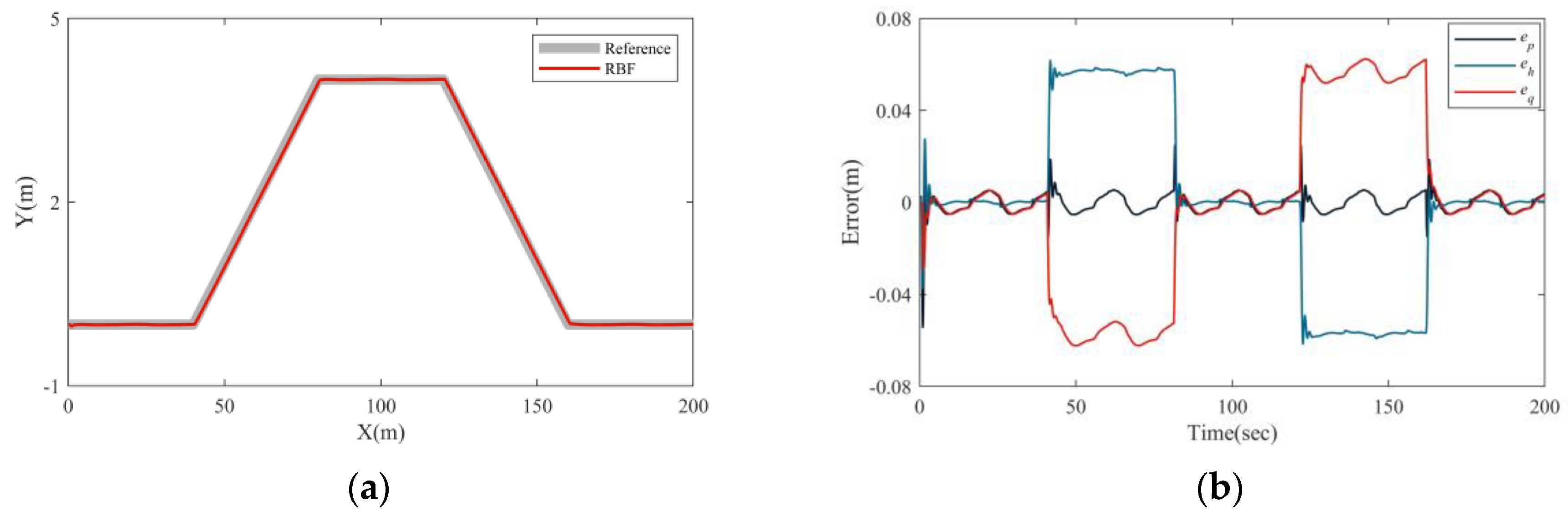
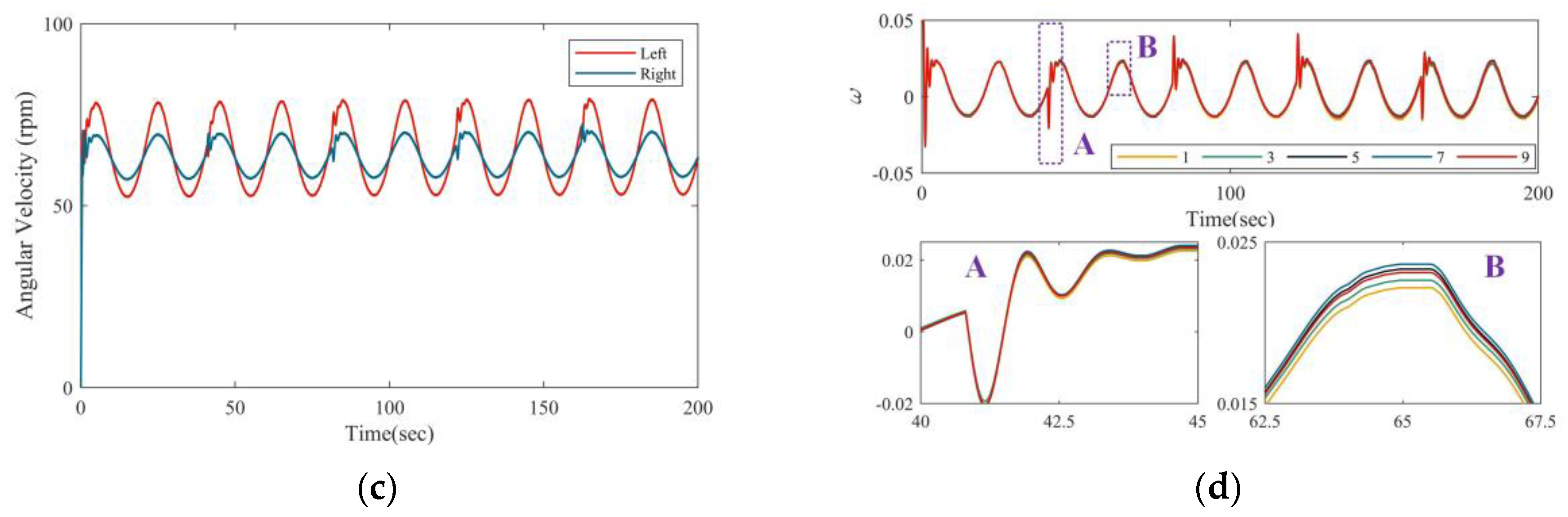
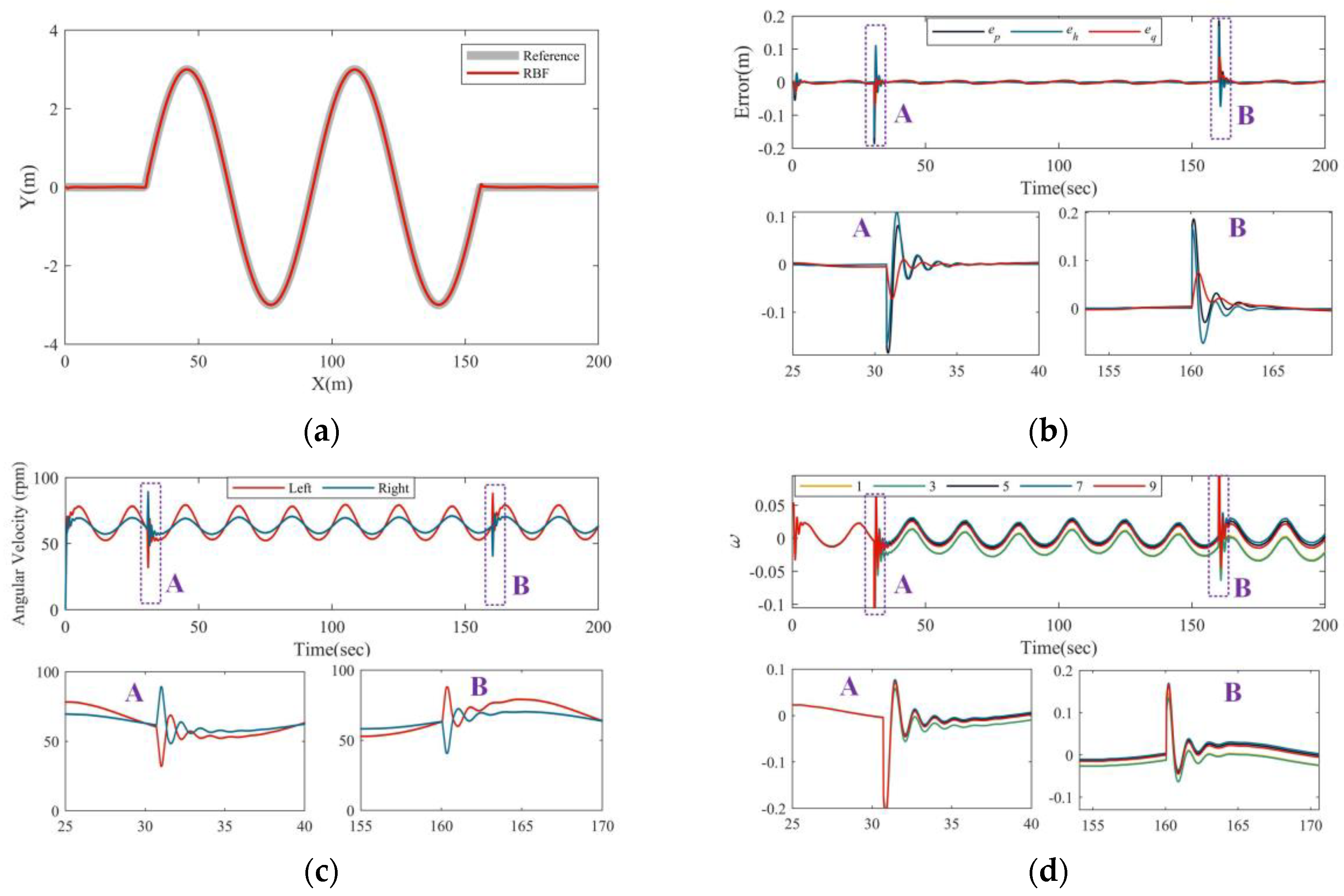
Figure 6 and Figure 7 show the results of the proposed control framework by tracking a DLC and a snaking path, respectively. The wheeled robot controlled by the proposed framework can track both reference paths precisely without any significant offset from the “reference”, and these are shown in Figure 6a and Figure 7a. Position and orientation errors, as well as the equivalent tracking error when tracking the reference paths, are illustrated in Figure 6b and Figure 7b. The maximum position error of the proposed framework was less than 0.08 m when tracking a DLC path, and it occurred in the lane-change part. The equivalent error remained at nearly zero during the tracking process, which indicates the effectiveness of the RBF network in reducing error indicators (Equation (20)). In contrast, sharp increases in errors occurred when tracking a snaking path. The reference snaking path was composed of two straight lines and a sinusoid, and abrupt changes in the reference orientation are occurred the intersections of the straight line and curve. Although the tracking error increased to about 0.2 m when changing from a straight line to a sinusoid, it rapidly converged to zero.
Figure 6c and Figure 7c illustrate the angular velocities of the left and right driving wheels generated by the proposed control framework. Their periodic variations are due to slippage disturbance, as shown in Figure 5. The weighting coefficients of the output layer from neurons No. 1, 3, 5, 7, and 9 were selected and shown in Figure 6d and Figure 7d. These coefficients also varied with the slippage to achieve a lower evaluation indicator, while they showed abrupt increases and decreases in the discontinuous position of the reference paths. The results indicate that the proposed control framework can adapt to slippage disturbance in terms of adjusting the weights of the network. It can also adapt to the abrupt change in reference orientation. The adaptiveness and effectiveness of the proposed control framework were verified.
4.2. Comparison with Other Control Algorithms
In this paper, a single neuron network (SNN) [27] and a PID control algorithms were selected for comparisons with the proposed control framework in order to demonstrate the tracking performance. Equivalent error was also employed as the control target for the two controllers. The results of the three control algorithms to in tracking a DLC and a snaking reference path under slippage disturbance are shown in Figure 8.
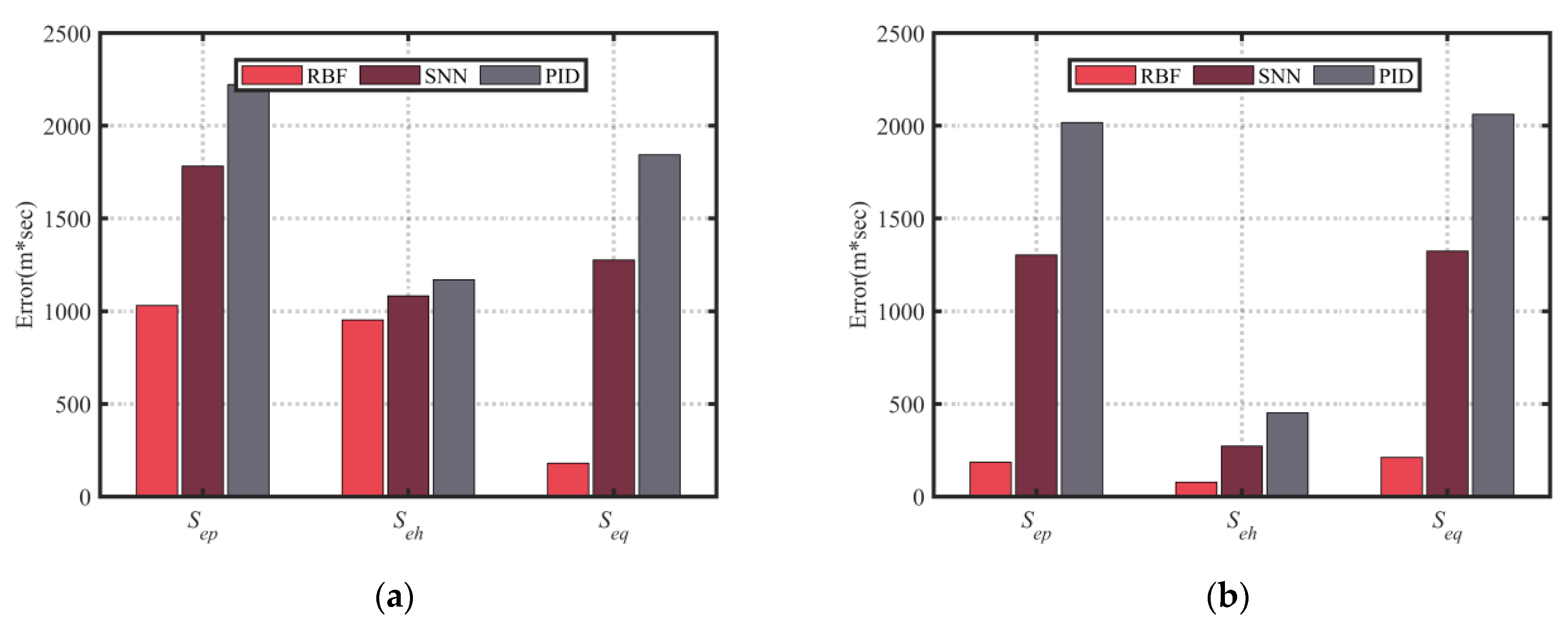
A quantification method was employed to evaluate the path tracking performance of the different algorithms. Accumulate position, orientation and equivalent errors during the tracking process, denoted by , , and , respectively, are defined as
where T is the total time of path tracking.
The trajectories and variations in the tracking errors with the time of the proposed control framework, SNN, and PID when tracking a DLC path are illustrated in Figure 8. The DLC path could be tracked by all of the afore-mentioned controllers. The variations in and of the PID and SNN controllers occurred in a larger range when compared with those of the proposed control framework. The maximum values of the PID and SNN controllers are nearly 0.15 m and 0.08 m, respectively, and they are much higher than those of the RBF. The swinging postures of the robot are exhibited in trajectories of the SNN and PID (Figure 8a), and this is due to the oscillating variations in of the two controllers in the tracking process (Figure 8b). Although the heading error remained nearly constant in the lane-changing process, the proposed framework yielded a steady posture.
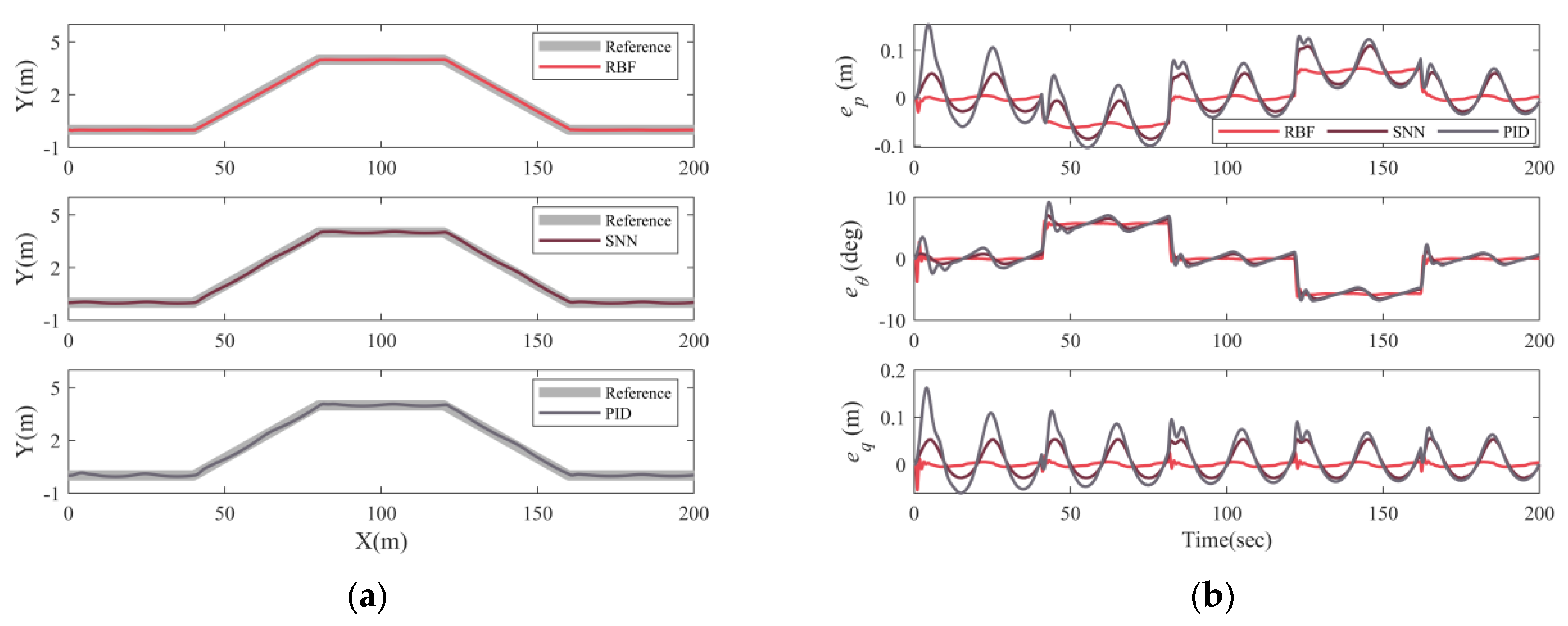
Figure 9 compares the results of three controllers by tracking a snaking target path. As shown in Figure 9a, a swinging posture of the wheeled robot appeared when tracking the straight-line part for the SNN and PID controllers. The three controllers yielded an abrupt increase in tracking errors in the intersections between a straight line and a sinusoid curve, which is illustrated in Figure 9b. The maximum values of the PID and SNN are about 0.18 m and 0.1 m, respectively, and they are much higher than those of the proposed framework. The obviously periodic changes in the three tracking errors of the SNN and PID were caused by slip ratio variations (Figure 5). The slippage disturbance led to degradation in the tracking performance of the SNN and PID controllers. The proposed control framework exhibited the lowest tracking errors and prior anti-disturbance performance when compared with those of the SNN and PID. The robot could track the target path with lower errors and a steady posture.
Figure 10 compares the accumulate position, orientation, and equivalent errors of three different controllers. The proposed framework yielded the lowest Sep, Seh, and Seq in both the DLC and snaking path tracking processes, while the PID controller exhibited much higher accumulate errors than those of the other controllers. As shown in Figure 10a, the proposed controller yielded much lower Seq than Sep and Seh when tracking the DLC path. This is because that the equivalent tracking error is defined by taking account for the position error of a future state and the heading error which may lead to approaching the target path, decreases . This integrated consideration of tracking error caused a decrease in the accumulate position error. Seh of the three controllers when tracking the DLC path is much higher than when tracking the snaking path, which is due to a steady heading error in the lane changing process, as shown in Figure 8b.
5. Conclusions
An adaptive path-tracking controller is proposed in this study to overcome slippage disturbances. Both a kinematic model and a dynamic model of a wheeled robot with skid-steer characteristics are established for the development of a dual-loop control framework. An RBF neural network is employed to design a yaw rate controller with anti-slippage performance. Simulations to track snaking and DLC paths are conducted under slippage disturbances. The proposed control framework yields much lower accumulate position, orientation, and equivalent tracking errors compared with those of an SNN and a PID controller. It also exhibits steady posture during the tracking process, which indicates its prior anti-slippage performance. The weights of the output layer in the RBF network vary with respect to the disturbances input. The proposed dual-loop controller is demonstrated to adapt to slippage, indicating that it could be employed in future vehicles or robots working in complex conditions. While the model did not consider the effect of vertical direction on path tracking. Our future work will focus on the validation of the proposed control framework in a field environment with complex terrain and take into account the vertical stiffness of the tire model.
Author Contributions
Conceptualization, Y.K. and R.Z.; methodology, Y.K. and B.X.; software, Y.K.; validation, Y.K., B.X. and R.Z.; formal analysis, B.X.; investigation, R.Z.; resources, Y.K.; data curation, R.Z.; writing—original draft preparation, Y.K. and B.X.; writing—review and editing, Y.K. and B.X.; visualization, B.X.; supervision, Y.K. and R.Z.; funding acquisition, Y.K. All authors have read and agreed to the published version of the manuscript.
Funding
This research was funded by Natural Science Foundation of China under grant number 51804019, Youth Core Individuals Project of Beijing under grant number 2017000020124G022, Fundamental Research Funds for the Central Universities under grant number FRF-TP-18-010A2 and National Key Research and Development Plan program under grant number 2018YFC0604402.
Institutional Review Board Statement
Not applicable.
Informed Consent Statement
Not applicable.
Data Availability Statement
Not applicable.
Conflicts of Interest
The authors declare no conflict of interest.
References
- Amer, N.H.; Zamzuri, H.; Hudha, K. Modelling and Control Strategies in Path Tracking Control for Autonomous Ground Vehicles: A Review of State of the Art and Challenges. J. Intell. Robot. Syst. 2016, 86, 1–30. [Google Scholar] [CrossRef]
- Tavan, N.; Tavan, M.; Hosseini, R. An optimal integrated longitudinal and lateral dynamic controller development for vehicle path tracking. Latin Am. J. Solids Struct. 2014, 12, 1006–1023. [Google Scholar] [CrossRef]
- Guo, L.; Ge, P.S.; Yang, X.L. Intelligent vehicle trajectory tracking based on neural networks sliding mode control. In Proceedings of the International Conference on Informative and Cybernetics for Computational Social Systems IEEE, Qingdao, China, 9–10 October 2014. [Google Scholar]
- Yue, M.; Wang, L.; Ma, T. Neural network based terminal sliding mode control for WMRs affected by an augmented ground friction with slippage effect. IEEE/CAA J. Autom. Sin. 2017, 4, 498–506. [Google Scholar] [CrossRef]
- Huynh, H.N.; Verlinden, O.; Wouwer, A.V. Comparative application of model predictive control strategies to a wheeled mobile robot. J. Intell. Robot. Syst. 2017, 87, 81–95. [Google Scholar] [CrossRef]
- Hernandez-Guzman, V.M.; Silva-Ortigoza, R.; Marquez-Sanchez, C. A PD path-tracking controller plus inner velocity loops for a wheeled mobile robot. Adv. Robot. 2015, 29, 1015–1029. [Google Scholar] [CrossRef]
- Park, M.; Lee, S.; Han, W. Development of Steering Control System for Autonomous Vehicle Using Geometry-Based Path Tracking Algorithm. Etri J. 2015, 37, 617–625. [Google Scholar] [CrossRef]
- Rajamani, R.; Zhu, C.; Alexander, L. Lateral control of a backward driven front-steering vehicle. Control Eng. Pract. 2003, 11, 531–540. [Google Scholar] [CrossRef]
- Li, Z.; Xu, C. Adaptive fuzzy logic control of dynamic balance and motion for wheeled inverted pendulums. Fuzzy Sets Syst. 2009, 160, 1787–1803. [Google Scholar] [CrossRef]
- Li, Z.; Li, J.; Kang, Y. Adaptive robust coordinated control of multiple mobile manipulators interacting with rigid environments. Automatica 2010, 46, 2028–2034. [Google Scholar] [CrossRef]
- Wang, D.; Low, C.B. Modeling and analysis of skidding and slipping in wheeled mobile robots: Control design perspective. IEEE Trans. Robot. 2008, 24, 676–687. [Google Scholar] [CrossRef]
- Yoo, S.J. Adaptive neural tracking and obstacle avoidance of uncertain mobile robots with unknown skidding and slipping. Inf. Sci. 2013, 238, 176–189. [Google Scholar] [CrossRef]
- Kang, H.S.; Kim, Y.T.; Hyun, C.H. Generalized Extended State Observer Approach to Robust Tracking Control for Wheeled Mobile Robot with Skidding and Slipping. Int. J. Adv. Robot. Syst. 2013, 10, 463–474. [Google Scholar] [CrossRef]
- Gao, H.; Song, X.; Liang, D. Adaptive motion control of wheeled mobile robot with unknown slippage. Int. J. Control 2014, 87, 1513–1522. [Google Scholar] [CrossRef]
- Chen, C.; Gao, H.; Ding, L. Trajectory tracking control of WMRs with lateral and longitudinal slippage based on active disturbance rejection control. Robot. Auton. Syst. 2018, 107, 236–245. [Google Scholar] [CrossRef]
- Xuan, V.; Ha, C.; Lee, J. Fuzzy Vector Field Orientation Feedback Control-Based Slip Compensation for Trajectory Tracking Control of a Four Track Wheel Skid-Steered Mobile Robot. Int. J. Adv. Robot. Syst. 2013, 10, 1–14. [Google Scholar]
- Bayar, G.; Bergerman, M.; Konukseven, E.I. Improving the trajectory tracking performance of autonomous orchard vehicles using wheel slip compensation. Biosyst. Eng. 2016, 146, 149–164. [Google Scholar] [CrossRef] [Green Version]
- Han, J. Tracking Control of Moving Sound Source Using Fuzzy-Gain Scheduling of PD Control. Electronics 2020, 9, 14. [Google Scholar] [CrossRef] [Green Version]
- Helmick, D.M.; Cheng, Y.; Clouse, D.S. Path following using visual odometry for a mars rover in high-slip environments. Aerosp. Conf. Proc. IEEE 2004, 2, 772–789. [Google Scholar]
- Lucet, E.; Lenain, R.; Grand, C. Dynamic path tracking control of a vehicle on slippery terrain. Control Eng. Pract. 2015, 42, 60–73. [Google Scholar] [CrossRef]
- Taghavifar, H.; Rakheja, S. A novel terramechanics-based path-tracking control of terrain-based wheeled robot vehicle with matched-mismatched uncertainties. IEEE Trans. Veh. Technol. 2019, 69, 67–77. [Google Scholar] [CrossRef]
- Prado, Á.J.; Michałek, M.M.; Cheein, F.A. Machine-learning based approaches for self-tuning trajectory tracking controllers under terrain changes in repetitive tasks. Eng. Appl. Artif. Intell. 2018, 67, 63–80. [Google Scholar] [CrossRef]
- Huang, J.; Wen, C.; Wang, W. Adaptive output feedback tracking control of a nonholonomic mobile robot. Automatica 2014, 50, 821–831. [Google Scholar] [CrossRef]
- Li, Z.; You, B.; Ding, L. Trajectory Tracking Control for WMRs with the Time-Varying Longitudinal Slippage Based on a New Adaptive SMC Method. Int. J. Aerosp. Eng. 2019, 2019, 1–13. [Google Scholar] [CrossRef] [Green Version]
- Wang, Z.P.; Ge, S.S.; Lee, T.H. Adaptive neural network control of a wheeled mobile robot violating the pure nonholonomic constraint. In Proceedings of the 43rd IEEE Conference on Decision and Control, Atlantis, Paradise Island, Bahamas, 14–17 December 2004. [Google Scholar]
- Gao, Y.; Cao, D.; Shen, Y. Path-following control by dynamic virtual terrain field for articulated steer vehicles. Veh. Syst. Dyn. 2020, 58, 1528–1552. [Google Scholar] [CrossRef]
- Li, J.; Liu, X.; Liu, G. Application of an adaptive controller with a single neuron in control of multi-motor synchronous system. In Proceedings of the 2008 IEEE International Conference on Industrial Technology, Chengdu, China, 21–24 April 2008. [Google Scholar]
Figure 1.
Description of the kinematic model with error definition for path tracking.

Figure 2.
Dynamic model of a skid–steer wheeled robot.

Figure 3.
Configuration of the path tracking control framework.

Figure 4.
Scheme of the yaw rate controller based on an RBF neural network.

Figure 5.
Slip ratio variations of the left and right tracks.

Figure 6.
Tracking results of the proposed framework under a double-lane-change maneuver: (a) trajectory, (b) tracking errors, (c) angular velocity of the left and right driving wheels, and (d) weights of the RBF network.
Figure 6.
Tracking results of the proposed framework under a double-lane-change maneuver: (a) trajectory, (b) tracking errors, (c) angular velocity of the left and right driving wheels, and (d) weights of the RBF network.


Figure 7.
Tracking results of the proposed framework under a snaking path maneuver: (a) trajectory, (b) tracking errors, (c) angular velocity of the left and right driving wheels and (d) weights of the RBF network.
Figure 7.
Tracking results of the proposed framework under a snaking path maneuver: (a) trajectory, (b) tracking errors, (c) angular velocity of the left and right driving wheels and (d) weights of the RBF network.

Figure 8.
Comparison of results of different control algorithms by tracking a DLC path: (a) trajectory and (b) tracking errors.
Figure 8.
Comparison of results of different control algorithms by tracking a DLC path: (a) trajectory and (b) tracking errors.

Figure 9.
Comparison of results of different control algorithms in tracking a snaking path: (a) trajectory and (b) tracking errors.
Figure 9.
Comparison of results of different control algorithms in tracking a snaking path: (a) trajectory and (b) tracking errors.

Figure 10.
Comparison of accumulate errors of different control methods by tracking (a) a DLC path and (b) a snaking path.
Figure 10.
Comparison of accumulate errors of different control methods by tracking (a) a DLC path and (b) a snaking path.


Table 1.
Parameters of the robot model.
| Parameter | Value | Unit |
|---|---|---|
| r | 0.21 | m |
| B | 0.67 | m |
| m | 115 | kg |
| J | 20.59 | kgm2 |
| JL | 3.29 | kgm2 |
| JR | 3.29 | kgm2 |
| CxL | 10 | kN |
| CxR | 10 | kN |
| Cy | 240 | N (°)−1 |
| D | 0.5335 | Nm (A)−1 |
| Z | 0.005 | Nms (rad)−1 |
Publisher’s Note: MDPI stays neutral with regard to jurisdictional claims in published maps and institutional affiliations. |
© 2021 by the authors. Licensee MDPI, Basel, Switzerland. This article is an open access article distributed under the terms and conditions of the Creative Commons Attribution (CC BY) license (https://creativecommons.org/licenses/by/4.0/).
Share and Cite
MDPI and ACS Style
Kang, Y.; Xue, B.; Zeng, R. Self-Adaptive Path Tracking Control for Mobile Robots under Slippage Conditions Based on an RBF Neural Network. Algorithms 2021, 14, 196. https://0-doi-org.brum.beds.ac.uk/10.3390/a14070196
AMA Style
Kang Y, Xue B, Zeng R. Self-Adaptive Path Tracking Control for Mobile Robots under Slippage Conditions Based on an RBF Neural Network. Algorithms. 2021; 14(7):196. https://0-doi-org.brum.beds.ac.uk/10.3390/a14070196
Chicago/Turabian StyleKang, Yiting, Biao Xue, and Riya Zeng. 2021. "Self-Adaptive Path Tracking Control for Mobile Robots under Slippage Conditions Based on an RBF Neural Network" Algorithms 14, no. 7: 196. https://0-doi-org.brum.beds.ac.uk/10.3390/a14070196
Note that from the first issue of 2016, this journal uses article numbers instead of page numbers. See further details here.