
An Optimal and Stable Algorithm for Clustering Numerical Data


Faculty of Computer and Mathematical Sciences, Universiti Teknologi MARA (UiTM), Shah Alam 40450, Malaysia
*
Author to whom correspondence should be addressed.
Algorithms 2021, 14(7), 197; https://0-doi-org.brum.beds.ac.uk/10.3390/a14070197
Submission received: 25 May 2021
/
Revised: 22 June 2021
/
Accepted: 25 June 2021
/
Published: 29 June 2021
Abstract
:In the conventional k-means framework, seeding is the first step toward optimization before the objects are clustered. In random seeding, two main issues arise: the clustering results may be less than optimal and different clustering results may be obtained for every run. In real-world applications, optimal and stable clustering is highly desirable. This report introduces a new clustering algorithm called the zero k-approximate modal haplotype (Zk-AMH) algorithm that uses a simple and novel seeding mechanism known as zero-point multidimensional spaces. The Zk-AMH provides cluster optimality and stability, therefore resolving the aforementioned issues. Notably, the Zk-AMH algorithm yielded identical mean scores to maximum, and minimum scores in 100 runs, producing zero standard deviation to show its stability. Additionally, when the Zk-AMH algorithm was applied to eight datasets, it achieved the highest mean scores for four datasets, produced an approximately equal score for one dataset, and yielded marginally lower scores for the other three datasets. With its optimality and stability, the Zk-AMH algorithm could be a suitable alternative for developing future clustering tools.

1. Introduction
Clustering or cluster analysis [1,2,3,4] is an unsupervised classification method that does not require object labeling during clustering [2,5,6,7]. Many clustering approaches, such as hierarchical clustering, partitional clustering, mixture density-based clustering, graph-theoretic clustering, fuzzy clustering, and search technique-based clustering, are being actively developed for various cluster analysis applications. One of the most efficient clustering approaches, particularly for clustering large and high-dimensional datasets, is partitional clustering [2]. This approach involves estimating the center of a cluster, optimizing an objective function, and finally assigning objects to clusters based on their distances to the centers of the clusters. Formally, partitional methods address the problem of dividing n cases, described by p variables, into a small number k of discrete classes [8]. Two popular heuristic methods are often adopted in this approach: centroid-based techniques such as the k-means and fuzzy c-means algorithms, as well as the k-modes and fuzzy k-modes approaches; and representative object-based techniques, such as the k-medoid method [6,9]. In general, in partitional algorithms, the center can be the mean, mode, median, or object itself.
The k-means clustering algorithm [10] is the precedent for several recent partitional algorithms. Numerous algorithms have been derived from the k-means framework, including fuzzy approaches such as the fuzzy c-means algorithm [11], categorical approaches such as the k-modes [12] and fuzzy k-modes algorithms [13], and mixed-type approaches [14] such as k-prototypes algorithm [12] and several modified versions such as those reported in [15,16]. An alternative to k-means is the k-approximate modal haplotype (k-AMH) algorithm [17], which is specifically intended for Y-DNA short tandem repeats (Y-STR) clustering problems and derived from the k-means framework. This algorithm is similar to the k-means framework in terms of the seeding selection mechanism but uses a fuzzy partition matrix in its optimization process. The other difference is that its cluster center is based on objects such as k-medoids.
In the partitioning of algorithms such as k-means, the main problem with obtaining optimal clustering results lies in the seeding selection mechanism. In fact, the seeding process is the first step in the k-means clustering framework and is a primary contributor to the optimization process. It is well known that an appropriate seeding selection mechanism may produce optimal clustering results; accordingly, numerous investigations have been performed on this issue. One of the most popular seeding methods proposed to address this problem for the k-means algorithm is the k-means++ algorithm [18]. The k-means++ algorithm adopts a statistical probability popularly known as careful seeding in the seeding selection mechanism in the original k-means algorithm. This careful seeding process has also been inherited in the fuzzy clustering approach. The fuzzy c-means algorithm [11] uses a randomly generated fuzzy membership values to initialize a partition matrix for the seeding process; however, it is difficult to control the initialization seeding in this method to obtain the optimal solution, and the operations of this algorithm are quite complex [19]. The k-means++ algorithm, which is a similar seeding method, was simply incorporated into the fuzzy c-means approach to derive a new extension known as fuzzy c-means++ [20]. This attempt demonstrated a significant contribution to the overall performance of the fuzzy c-means method, particularly in terms of making the process less time consuming. Consequently, numerous seeding methods for the fuzzy c-means approach, e.g., mountain clustering [21], subtractive clustering [22,23], and grid and density clustering [19] were proposed.
The issue related to seeding selection continues to exist and has attracted a significant amount of research attention, and various ideas have been proposed over the past few years. For example, a new seeding approach called the k-centroid initialization algorithm (PkCIA) based on eigenvalues/eigenvectors for computing initial cluster centroids was recently proposed [24]. Another seeding selection mechanism was proposed based on a small subset of non-degenerate observation points extracted from an original dataset [25]. In addition, Franti and Sieranoja [26] conducted an intensive study on the seeding selection issue and split it into six categories: random points, farthest point heuristic, sorting heuristic, density-based, projection-based, and splitting technique; however, no clear conclusion was made as to which seeding method or category works better [26]. Therefore, further improvement of the seeding mechanism is needed, and attempts to achieve the required optimality, particularly for k-means is an ongoing research problem. In addition, to tackling seeding selection issues, a recent idea, aimed at optimal clustering results, is the repeated k-means. This method must be performed multiple times with different seeding selection mechanisms while maintaining the lowest SSE value [26]. At present, attempts are ongoing in this regard.
The k-AMH algorithm, however, seems to present a comparably less significant seeding selection issue. For example, the original k-AMH algorithm for categorical data was found to be superior to other extended k-means approaches such as the k-modes and fuzzy k-modes methods [17]. A key advantage of the k-AMH algorithm is that it provides a higher minimum accuracy score compared with the other algorithms, as determined by performing 100 experimental runs. Apparently, the main factor that contributes to its superiority over other algorithms is that the k-AMH framework is not heavily dependent on the seeding selection mechanism, even though it uses random seeds. This advantage also exists for the k-AMH numerical extensions, called k-AMH numeric I and II [27], and these approaches have been found to be comparable to the fuzzy c-means technique. An earlier attempt to improve the random seeding mechanism for the original k-AMH algorithm, in particular for Y-STR clustering, yielded very promising results [28].
The aforementioned points discussed above present a basis to employ the k-AMH framework in order to yield highly constant results for each seeding while still maintaining their optimality. As discussed above, numerous attempts at seeding, such as the popular k-means++ approach, seem to be primarily focused on obtaining optimal clustering results. This is because optimality is prioritized when solving clustering problems. Benchmarking the optimality is subject to certain comparisons with existing solutions or algorithms, particularly for k-means algorithm. Notably, very few studies on cluster stability have been conducted thus far. This can be attributed to the fact that cluster stability is required only after desirable optimality by the appropriate seeding selection mechanism. According to Franti and Sieranoja [26], k-means can be improved from two aspects: better initialization (Seeding selection) and repeated k-means. At present, no concrete solution has been obtained. For k-AMH algorithm, a recent attempt for the repeated k-AMH has been proposed [29]. This finding is quite promising; however, it must be noted that an optimal objective function is not necessarily produced optimal clustering results.
Clustering should be a structure on a dataset that is stable. When applied to several datasets from the same underlying model or of the same data-generating process, the clustering algorithm should yield similar results [30]. From an experimental perspective, clustering algorithms should produce optimal and stable results in every run; however, the seeding selection mechanism may vary, which may occasionally lead to different clustering results. Therefore, we herein introduces a new algorithm based on the k-AMH framework and associated with a simple but novel seeding mechanism, with the objective of achieving cluster optimality and stability. Clustering algorithms are made of a clear distinction between clustering method (objective function) and clustering algorithm (the framework) [1,31]; therefore, the proposed algorithm is based on the k-means objective function, combined with the k-AMH clustering framework and worked with a simple and novel seeding selection mechanism known as zero-point multidimensional spaces. The aim is to achieve optimality clustering along with stability. Cluster optimality and stability are defined as the capability of an algorithm to produce optimal results and stable results for every seeding and run. Therefore, the proposed algorithm, which has the advantages of optimality and stability, can serve as an alternative method for the repeated k-means approach.
2. Preliminaries
2.1. k-Means Clustering Framework
The traditional k-means algorithm is based on a center-based clustering framework [2] in which objects are partitioned into a cluster according to their distances to the cluster centers. Generally, the objective of k-means is to partition a dataset X into C cluster with the number of clusters, k, set as a priori. Let be a set of n objects and be represented with its attributes as . In addition, let be a set of k cluster centers and be represented with its attributes as . Finally, is a set of k clusters. Generally, using the k-means framework, X is partitioned into C through the following steps:
- Step 1—First, initialize the number of clusters, k.
- Step 2—Randomly select Z from X as the center of clusters (better known as centroids).
- Step 3—Assign X to the closest cluster centroid based on the distance of each X and Z. The distance is typically calculated using Euclidean distance as Equation (1).
- Step 5—Repeat Steps 3 and 4 and stop when the process intra- and inter-cluster dissimilarity objective function are minimized. The objective function is computed as in Equation (7)
For fuzzy approach, the algorithm is called fuzzy c-means algorithm and uses the same framework as above. However, the objective function is minimized as Equation (8),
which is subject to the following Equations (9)–(11),
where is a weighting exponent that is typically greater than 1.0. The partition matrix, also known as fuzzy membership, W, is updated as Equation (12)
and the centroid of fuzzy c-means is updated as Equation (13)
The fuzzy c-means algorithm can be formalized in the form of pseudocode as Algorithm 1.
| Algorithm 1 FUZZY C-MEANS (. |
|
Input: dataset X, number of clusters k, and weighting exponent Output: Set of clusters |
2.2. k-AMH Clustering Framework
Similar to k-Means, the k-AMH [17] uses the same clustering framework, which begins with random seeds and updating the centers of the clusters and ends with optimizing an objective function. Finally, the objects closer to the centers of the clusters are grouped together into those clusters. The k-AMH algorithm differs from the k-means algorithm in terms of how the centers are updated. The k-AMH algorithm exploits the objects themselves to update the cluster centers, whereas the fuzzy c-means algorithm uses the mean, as the name implies. In general, the k-AMH algorithm has two extensions: the k-AMH algorithm for categorical clustering, which is the original version previously introduced for clustering Y-STR data, and the recent k-AMH algorithm for numerical clustering. In addition, there are two extended versions of numerical clustering [27]. The first one follows the original k-AMH categorical algorithm exactly except that the numerical distance, e.g., Euclidean distance (previously reported as k-AMH numeric I), is used, whereas the second version has its objective function substituted with the objective function of the fuzzy c-means algorithm (previously reported as k-AMH numeric II).
2.2.1. k-AMH Algorithm for Categorical Clustering
As mentioned above, the k-AMH algorithm [17] for categorical clustering is the original k-AMH algorithm. Beginning with predefined k clusters, k seeding is initialized, the objects are tested individually, and the objects are replaced in succession to obtain the final objects as the centers of the clusters. Let be a set of n categorical objects and be a set of objects at the centers of clusters, better known as medoids. To partition X into C, the k-AMH framework generally requires the following steps:
- Step 1—First, initialize the number of clusters, k.
- Step 2—Randomly select H from X as the center of the clusters (better known as medoids).
is maximized and defined in Equation (15):
where is a matrix and is another matrix containing the dominant weighting value.
The describes the degree of fuzziness of the object, which contains values from 0 to 1, as described in Equation (16).
where is a predefined number of clusters, H is the medoid such that is a weighting exponent that is typically greater than 1.0, and is the dissimilarity measure calculated between object and medoid , as described in Equation (17):
where m is the number of attributes and subject to the following conditions,
The assigns a value of 1.0 or 0.5, known as the dominant weighting value, as described in Equation (19):
which is subject to the following Equations (20) and (21),
- Step 4—Assign X to C when the final H is obtained.
Thus, the procedure above can be formalized in the form of pseudocode as Algorithm 2.
| Algorithm 2 k-AMH (. |
|
Input: dataset X, number of clusters k, and weighting exponent Output: Set of clusters |
2.2.2. k-AMH Algorithm for Numerical Clustering
This section provides the procedure of the k-AMH numerical algorithm for numerical clustering. k-AMH numeric II [27] was chosen as the algorithm to be used for the new seeding mechanism. Please note that k-AMH numeric I could not be used in this case due to the maximization procedure. Similarly, k-AMH numeric II (simply called the k-AMH numeric hereafter) requires the testing and replacement of objects if and only if the objective function is minimized. Please note that this k-AMH numerical algorithm, the objective function is not based on a maximization process as imposed by the original k-AMH algorithm. Therefore, the k-AMH numeric algorithm follows exactly the original k-AMH steps above except for Step 3 which is the updating medoids, the k-AMH numeric replacement’s object is based on the objective function as described in Equation (8). To partition X into C, the k-AMH numeric framework generally requires the following steps:
- Step 1—First, initialize the number of clusters, k.
- Step 2—Randomly select Z from X as the center of the clusters (better known as medoids).
- Step 3—Replace the medoids, Z, by testing each one until . The updates are complete when the objective function is minimized as Equation (22).
- Step 4—Assign X to C when the final Z is obtained.
The procedure above can be formalized in the form of pseudocode as Algorithm 3.
| Algorithm 3 k-AMH NUMERIC (. |
|
Input: dataset X, number of clusters k, and weighting exponent Output: Set of clusters |
3. Proposed Clustering Algorithm with a Constant Seeding Selection
3.1. Proposed Seeding Selection Method
Traditionally, seeding selection for clustering algorithms, such as the k-means, k-modes, and fuzzy c-means algorithms, including the k-AMH algorithm, involves randomly generated seeds by default. Unlike the k-means framework, the k-AMH algorithm exploits the k-objects (usually known as medoids) from the seeding process until they are clustered. Thus, each object needs to be replaced individually to find the final k-objects if the objective function is optimized. For object replacement, the objective function minimization is mainly based on the minimization process of each set of k-objects forming a k-combination. Therefore, an appropriate combination of k-objects may lead to better clustering results and vice versa.
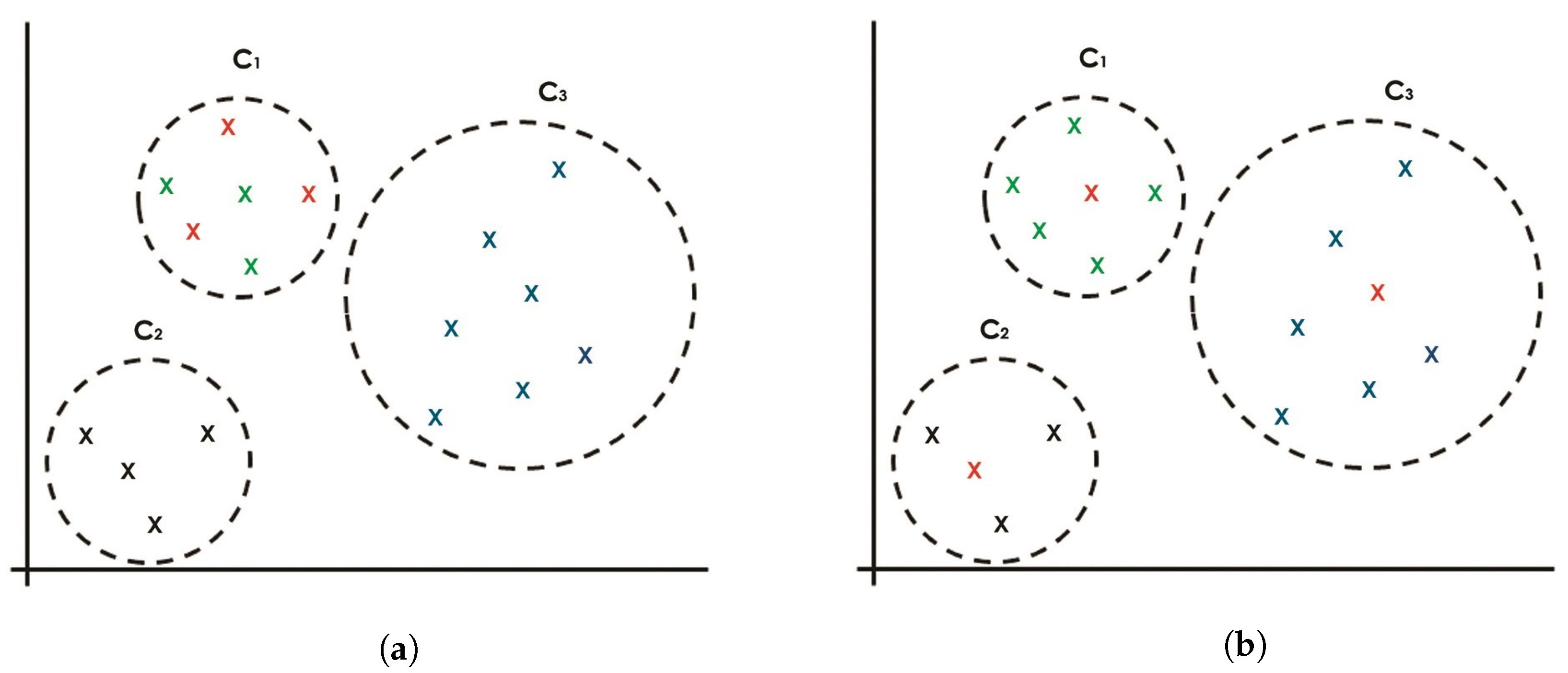
Figure 1 depicts two scenarios that may happen in the random seeding method. Consider three clusters and with objects colored in green, black, and blue, respectively, and the seeding of k-objects () that are taken from the objects randomly, represented in red. It is a well-known problem that many cases result in the worst-case scenario shown in Figure 1a, in which the three objects are seeded from the same cluster (the green cluster). However, it may also result in the best-case scenario shown in Figure 1b, in which the three objects are seeded and represented by each cluster. These scenarios may lead to either poorer clustering results (the worst-case scenario) or better clustering results (the best-case scenario). Therefore, for every run, the clustering results may vary, ranging from the worst-case to the best-case clustering performance.
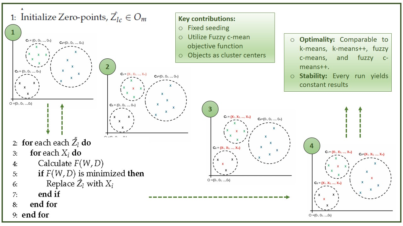
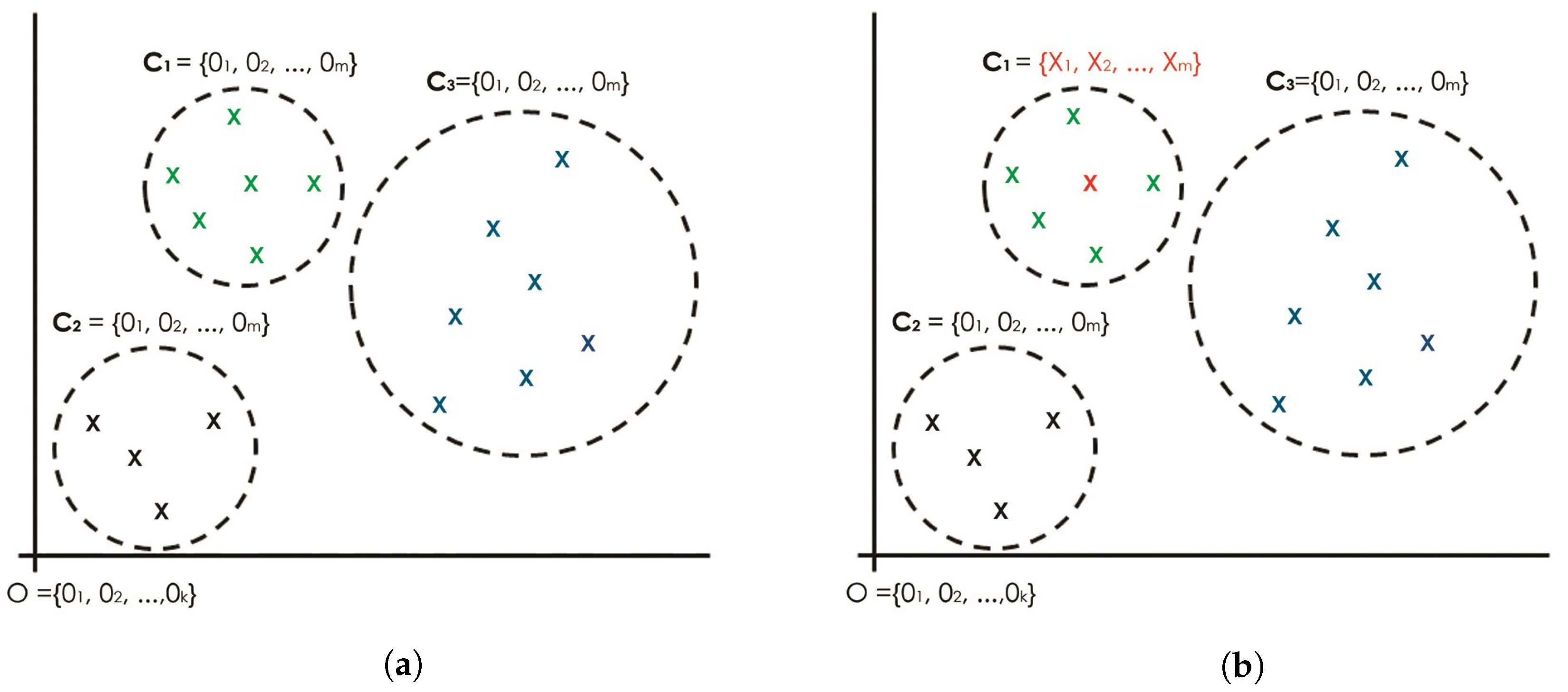
Roughly speaking, the proposed seeding concept is derived from a special point in a Cartesian coordinate system called the origin. Figure 2 depicts a conceptual idea of a new seeding mechanism that seeds the k-AMH algorithm with zero-point multidimensional spaces for each k-cluster.
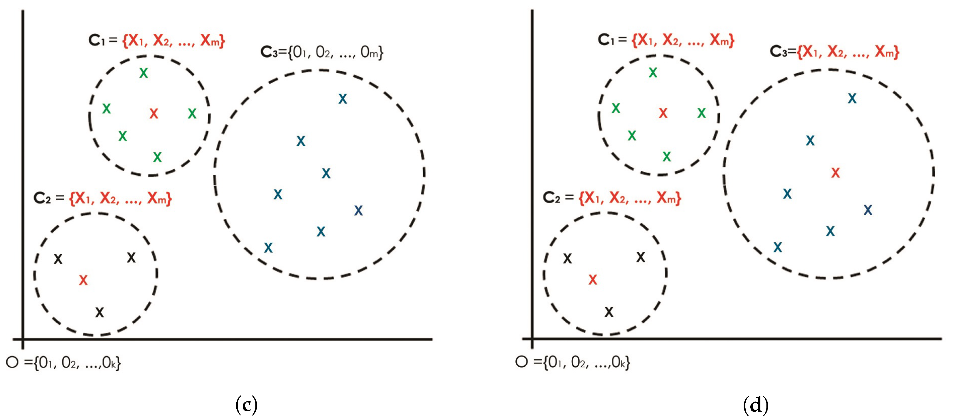
The idea is to offer a globally optimal solution for each object by pointing to the same data point, known as the origin shown in Figure 2a. In this process, selecting the k-objects seem to be more appropriate in setting up the best possible k-object combination shown in Figure 2d. Using the same k-AMH (numerical) framework, the proposed approach begins with the first k-object and testing of the objects individually to determine the object that will serve as the center of the first cluster, whereas the other clusters continue pointing to the origin, as shown in Figure 2b. This process is repeated for the second k-object shown in Figure 2c, then for the third k-object shown in Figure 2d. Under these circumstances, it is believed that the k-AMH algorithm converges in a globally optimal fashion for the best possible combination of k-objects. In fact, using the fixed reference point for every seeding process gives the new seeding method and k-AMH numeric algorithm the advantage of producing constant results. In such convergence spaces, the clustering results may reach stability and the optimal clustering results may be achieved in every run.
3.2. Proposed Algorithm
We call the new algorithm with zero-point seeding the Zk-AMH algorithm. The main difference between the Zk-AMH algorithm and the k-AMH numeric algorithm is the replacement of random seeding with zero-point multidimensional seeding. In addition, from an implementation perspective, each k-object will be compared to n objects rather than objects, as imposed by the original k-AMH numeric algorithm. This difference exists because the seeding objects are not taken from the n objects. Thus, the Zk-AMH algorithm employs the procedure and steps as described for the k-AMH numeric algorithm above exactly, except in terms of the seeding selection (Step 2). From the perspective of implementation, the zero-seeding assigns zero values of multidimensional spaces (attributes). Therefore, let be a set of origins and , where , and is the zero-seeding assigned to each with O. For example, if and , the initial seeding may resemble , , and . Therefore, the initial objective function as Equation (8) is first obtained by calculating the distance X and as Equation (1), which is based on the zero-seeding. This initial objective function must be maximal according to our theorem below.
Theorem 1.
Let be the zero-seeding for . is replaced with for to serve as the medoid if and only if
Proof.
Let be a set of n objects, be a set of zero-point seeding, and be a set of medoids (centers of clusters) for k clusters. Let be the distance between object and zero-seeding , and let ) be the distance between object and medoid . Thus, based on Equation (1), is given by
and is given by
Therefore, must be greater than . We write , where , and , where , as
As is greater than and and are non-negative, the product must be less than . It follows that the sum of all quantities obeys
Hence, the function is minimized, and the result follows. The convergence of the k-AMH algorithm is already proven based on that of the previous version [17].
Thus, the object replaced by testing one-by-one object as required by the k-AMH procedure, will yield the minimization process of the objective function. As a result, the final objects (medoids) are obtained after all the objects are tested and replaced accordingly. Based on the k-AMH procedure, the final medoids are the cluster centers that would achieve cluster optimality and stability. The zero-seeding that acts as fixed seeding selection leads to Zk-AMH stability.
Therefore, to partition X into C, the Zk-AMH algorithm requires the following steps:
- Step 1—First, initialize the number of clusters, k.
- Step 2—Select as the center of the clusters (better known as medoids).
- Step 4—Assign X to C when the final is obtained.
Therefore, the Zk-AMH algorithm can be described in pseudocode as Algorithm 4. □
3.3. Computational Complexity
In terms of the overall computational complexity, the Zk-AMH algorithm is linearly proportional to the size of the dataset with , where k is the number of clusters, m is the number of dimensional spaces, and n is the number of objects. The time taken for the new seeding is considered to be because the seeding is assigned once for the initialization. It is nearly similar to the computational complexity of the k-means algorithm, which is , where n is the number of objects, k is the number of clusters, and t is the number of iterations required for its iteration processes. The detailed time complexity and scalability testing for the k-AMH algorithm is reported in [17].
| Algorithm 4 Zk-AMH(. |
|
Input: dataset X, number of clusters k, and weighting exponent Output: Set of clusters |
4. Experimental Setup
4.1. Dataset
Eight real-world numerical datasets were used to evaluate the algorithm performance: the Iris, Pima, Haberman, Wine, Seed, User Knowledge, E-coli, and Cleveland datasets from the UC Irvine (UCI) machine learning repository [32]. The experiments were focused on measuring the cluster optimality and stability of the newly proposed algorithm. These datasets cover various scenarios such as number of attributes, ranging from 3 to 13, and the number of classes, ranging from 2 to 8. Table 1 summarizes the datasets used in this experiment.
4.2. Evaluation Method
A 100-run experiment was conducted for each algorithm and dataset for further analysis. On top of the proposed algorithm (the Zk-AMH), the other six algorithms were used for comparison. Table 2 lists and summarizes the algorithms.
An external criterion was used to evaluate the clustering performance. It can be used to discover inherent data structures in the clustering results [1] and measures the degree of correspondence between the clusters and the priori classes assigned to them. The Fowlkes-Mallows (FM) Index [33] was used to measure the performance of clustering algorithms as Equation (12)
where is the number of true positives, is the number of false positives, and is the number of false negatives.
5. Results
This section presents the results obtained from 100 experimental runs for each of the seven algorithms and eight datasets. The experimental results provide evidence that the new Zk-AMH seeding algorithm performs better than the existing algorithms. Based on the experimental results, the results of the analysis focus on two main factors according to the objectives stated earlier. First, to provide evidence that the new Zk-AMH seeding algorithm is optimal (Cluster optimality). This is the first goal that is primarily required for any new clustering algorithm. Second, to provide evidence that the Zk-AMH is stable (Cluster stability). Hence, FMI scores such as the mean, maximum, minimum, and standard deviation were chosen to compare the clustering performance of the Zk-AMH approach with respect to the six algorithms as listed in Table 2. Please note that for fuzzy clustering algorithms such as the fuzzy c-means, fuzzy c-means++, k-AMH, k-AMH++, and Zk-AMH algorithms, the weighting exponent of was set to 1.1.
5.1. Cluster Optimality
Figure 3 shows an initial comparison of the seven algorithms for the combination of the eight datasets considered. These results demonstrate that the Zk-AMH algorithm is certainly competitive and comparable to its counterparts, the k-means, k-means++, fuzzy c-means, fuzzy c-means++, k-AMH numeric, and k-AMH numeric++ algorithms. Overall, the Zk-AMH approach produced the highest minimum scores and marginally lower maximum scores than the other algorithms. Moreover, the box plot for the Zk-AMH algorithm is larger than those of the other algorithms, particularly in the third quartile. It indicates that the Zk-AMH algorithm attained scores that were greater than the median score and close to the maximum score as compared to the other algorithms.
Since the above results indicate that the proposed approach is very competitive, a one-way ANOVA was conducted to support these results. The test indicated that the assumption of homogeneity of variance was violated; therefore, the Welch F-ratio was reported. There was also significant variance in the clustering scores among the seven algorithms, in which . Thus, the Games–Howell post hoc test was used to compare the seven algorithms.
Table 3 compares the results of the Games–Howell post hoc test for the Zk-AMH algorithm with those for the other six algorithms. At the significance level and with , the mean score of the Zk-AMH algorithm ( confidence interval differs from those of the k-means ( confidence interval and k-means++ ( confidence interval ) algorithms. Thus, the k-AMH algorithm outperformed the k-means and k-means++ algorithms in terms of clustering performance. Furthermore, with , the performance of the Zk-AMH approach is essentially comparable to those of the fuzzy c-means ( confidence interval , fuzzy c-means++ ( confidence interval , k-AMH numeric ( confidence interval , and k-AMH numeric++ ( confidence interval algorithms in terms of average clustering performance.
Based on the overall average scores for the combination of all eight datasets, the results provide evidence that the Zk-AMH algorithm is optimal and comparable to the other clustering algorithms. The box plot demonstrated the first piece of evidence in this regard, where the Zk-AMH approach yielded the median value that is almost similar to the other algorithms, such as the fuzzy c-mean and k-AMH algorithms (see Figure 3). Furthermore, the Zk-AMH scored the highest minimum score in 800 experimental runs (1 algorithm × 100 runs × 8 datasets). Finally, the one-way ANOVA test proved that the Zk-AMH algorithm (a) outperformed the hard clustering approaches such as the k-means and k-means++ algorithms, (b) is comparable to the fuzzy c-means and fuzzy c-means++ approaches, and (c) retained its clustering performance with the original k-AMH algorithm and k-AMH with k-means++ seeding method (k-AMH++). In addition, for the dataset comparison, the Zk-AMH algorithm clearly showed its advantages by producing the highest scores for four datasets, an approximate score for one dataset, and marginally lower values for the other three datasets (see Table 4).
5.2. Cluster Stability
Table 4 presents the performances of all algorithms using the mean, maximum, minimum, and standard deviation. The values in bold are the optimum values (the highest minimum and maximum accuracies and lowest standard deviations) obtained by a particular algorithm for each dataset. The most impressive result regarding the Zk-AMH algorithm is that its standard deviation is zero for all datasets, which means that the mean, minimum, and maximum scores are identical. Based on this result, it can be concluded that the Zk-AMH algorithm produced constant and stable clustering results for every run. The other algorithms show their variability in producing clustering results due to seeding mechanism, even though they were seeded by distinctive objects as in k-means++ seeding. In addition, the Zk-AMH algorithm yielded the highest mean scores for four of the eight datasets, specifically, datasets 1, 4, 7 and 8; approximately the same mean score for dataset 5; and marginally lower mean accuracies for datasets 2, 3 and 6. Furthermore, the Zk-AMH algorithm produced the highest minimum score for all datasets except dataset 5, which had a marginally lower score. The Zk-AMH algorithm also demonstrated its competitiveness compared with the other six algorithms with marginally lower maximum scores.
6. Discussion
The first consideration regarding the Zk-AMH algorithm is the cluster optimality. Based on the overall average scores for the combination of all eight datasets, the results provide evidence that the Zk-AMH algorithm is optimal and comparable to the other clustering algorithms. The box plot demonstrated the first piece of evidence in this regard, where the Zk-AMH approach yielded approximately similar median value with the k-AMH, k-AMH++, and fuzzy c-means scores (see Figure 3). Furthermore, the Zk-AMH scored the highest minimum score in 800 experimental runs (1 algorithm × 100 runs × 8 datasets). Finally, the one-way ANOVA test proved that the Zk-AMH algorithm is optimal and comparable to the fuzzy c-means and fuzzy c-means++ approaches. In addition, for the dataset comparison, the Zk-AMH algorithm clearly showed its advantages by producing the highest scores for four datasets, an approximately score for one dataset, and marginally lower values for the other three datasets (see Table 4).
The second consideration regarding the Zk-AMH algorithm is the cluster stability. Most impressively, the Zk-AMH algorithm exhibited its strength by producing identical mean, minimum, and maximum scores, which led its standard deviation to decline to zero for all datasets (see Table 4). It is clearly evident that in the 100-run experiment for each dataset, the Zk-AMH managed to produce constant results. This scenario did not happen to the other algorithms, except for the fuzzy c-mean algorithm with dataset 5 alone. In fact, out of eight datasets, four produced the optimal values, whereas the other four datasets produced marginally lower scores. Further investigation of why these two datasets were less optimal is urgently required.
Hence, the new seeding method seems to be exceptionally well suited and to work exclusively for the k-AMH clustering framework to achieve cluster optimality and stability. The new seeding might not work for the k-means and fuzzy c-means frameworks due to their center using the mean. The cluster optimality is actually inherited from the previous performance of k-AMH framework. Furthermore, the new seeding mechanism contributed to cluster stability. With the fixed seeding technique and using multidimensional zero points (the origin), the Zk-AMH algorithm converges in a globally optimal fashion toward better clustering performance.
7. Conclusions
Based on the experimental results above, the Zk-AMH algorithm is stable while seeding with zero-point multidimensional Cartesian spaces. In fact, the algorithm also maintains its optimal solution for numerical clustering and is comparable not only to its original algorithm, the k-AMH numeric algorithm and its extension k-AMH numeric++, but also its counterparts, the k-means, k-means++, fuzzy c-means, and fuzzy c-means++ algorithms. The most promising finding is that the Zk-AMH algorithm obtained identical results for all datasets in every run, due to its cluster stability. Thus, the seeding selection would no longer be an obstacle to producing optimal clustering results for every run. With its optimality and stability, the proposed Zk-AMH has the potential to be used in the future development of clustering tools, particularly for numerical clustering.
Author Contributions
Conceptualization and Algorithm design, A.S.; Implementation and Analysis, A.M.S. Both authors have read and agreed to the published version of the manuscript.
Funding
This research received no external funding.
Institutional Review Board Statement
Not Applicable.
Informed Consent Statement
Not Applicable.
Data Availability Statement
The datasets used in this study are taken from UCI Machine Learning Repository.
Acknowledgments
We would like to thank the Dean, Haryani Haron for supporting us in completing this study.
Conflicts of Interest
The authors declare no conflict of interest.
References
- Jain, A.K.; Dubes, R.C. Algorithm for Clustering Data; Prentice Hall Inc.: Hoboken, NJ, USA, 1988. [Google Scholar]
- Gan, G.; Ma, C.; Wu, J. Data Clustering: Theory, Algorithms, and Applications; Society for Industrial and Applied Mathematics: Philadelphia, VA, USA, 2007. [Google Scholar]
- Jain, A.K.; Murthy, M.N.; Flynnand, P.J. Data clustering: A review. ACM Comput. Surv. 1999, 31, 264–323. [Google Scholar] [CrossRef]
- Kaufman, L.; Rousseeuw, P.J. Finding Groups in Data: An Introduction to Cluster Analysis; Wiley and Sons: New York, NY, USA, 1990. [Google Scholar]
- Xu, R.; Wunsch, D. Clustering; John Wiley and Sons: Hoboken, NJ, USA, 2009. [Google Scholar]
- Tan, T.; Steinbach, M.; Kumar, V. Introduction to Data Mining; Pearson Education, Inc.: Boston, MA, USA, 2006. [Google Scholar]
- Everitt, B.; Landau, S.; Leese, M. Cluster Analysis; Arnold: London, UK, 2001. [Google Scholar]
- Fielding, H. Cluster and Classification Techniques for Biosciences; Cambridge University Press: Cambridge, UK, 2007. [Google Scholar]
- Han, J.; Kamber, M. Data Mining: Concepts and Techniques; Morgan Kaufmann Publishers Inc.: San Francisco, CA, USA, 2001. [Google Scholar]
- MacQueen, J.B. Some methods for classification and analysis of multivariate observations. In 5th Berkeley Symposium on Mathematical Statistics and Probability; University of California Press: Berkeley, CA, USA, 1967; pp. 281–297. [Google Scholar]
- Bezdek, J.C. Pattern Recognition with Fuzzy Objective Function Algorithms; Plenum: New York, NY, USA, 1981. [Google Scholar]
- Huang, J.Z. Extensions to the k-means algorithm for clustering large data sets with categorical values. Data Min. Knowl. Discov. 1998, 2, 283–304. [Google Scholar] [CrossRef]
- Huang, J.Z.; Ng, M.K. A fuzzy k-modes algorithm for clustering categorical data. IEEE Trans. Fuzzy Syst. 1999, 7, 46–452. [Google Scholar]
- Caruso, G.; Gattone, S.A.; Balzanella, A.; Di Battista, T. Cluster Analysis: An Application to a Real Mixed-Type Data set. In Models and Theories in Social Systems. Studies in Systems, Decision and Control; Flaut, C., Hošková-Mayerová, Š., Flaut, D., Eds.; Springer: Cham, Switzerland, 2019; Volume 179, pp. 525–533. [Google Scholar]
- Alibuhtto, M.C.; Mahat, N.I. New approach for finding number of clusters usingdistance based k-means algorithm. Int. J. Eng. Sci. Math. 2019, 8, 111–122. [Google Scholar]
- Xie, H.; Zhang, L.; Lim, C.P.; Yu, Y.; Liu, C.; Liu, H.; Walters, J. Improving k-means clustering with enhanced firefly. Algorithms Appl. Soft Comput. 2019, 84, 105763. [Google Scholar] [CrossRef]
- Seman, A.; Bakar, Z.A.; Isa, M.N. An efficient clustering algorithm for partitioning y-short tandem repeats data. BMC Res. Notes 2012, 5, 1–13. [Google Scholar] [CrossRef] [PubMed] [Green Version]
- Arthur, D.; Vassilvitskii, S. k-means++: The advantages of careful seeding. In Proceedings of the Eighteenth Annual ACM-SIAM Symposium on Discrete Algorithms, New Orleans, LA, USA, 7–9 January 2007; pp. 1027–1035. [Google Scholar]
- Zou, K.; Wang, Z.; Pei, S.; Hu, M. An New Initialization Method for Fuzzy c-Means Algorithm Based on Density. In Fuzzy Information and Engineering. Advances in Soft Computing; Cao, B., Zhang, C., Li, T., Eds.; Springer: Berlin/Heidelberg, Germany, 2009. [Google Scholar]
- Stetco, A.; Zeng, X.-J.; Keane, J. Fuzzy c-means++: Fuzzy c-means with effective seeding initialization. Expert Syst. Appl. 2015, 42, 7541–7548. [Google Scholar] [CrossRef]
- Ronald, Y.; Filev, R.; Dimitar, P. Approximate clustering via the mountain method. IEEE Trans. Syst. Man Cybern. 1994, 24, 1279–1284. [Google Scholar]
- Chiu, S.L. Fuzzy model identification based on cluster estimation. J. Intell. Fuzzy Syst. 1994, 2, 267–278. [Google Scholar] [CrossRef]
- Pei, J.; Fan, J.; Xie, W. An initialization method of cluster centers. J. Electron. Sci. 1999, 21, 320–325. [Google Scholar] [CrossRef]
- Manochandar, S.; Punniyamoorthy, M.; Jeyachitra, R.K. Development of new seed with modified validity measures for k-means clustering. Comput. Ind. Eng. 2020, 141, 106290. [Google Scholar] [CrossRef]
- Zhang, X.; He, Y.; Jin, Y.; Qin, H.; Azhar, M.; Huang, J.Z. A robust k-means clustering algorithm based on observation point mechanism. Hindawi Complex. 2020, 2020, 3650926. [Google Scholar] [CrossRef]
- Fränti, P.; Sieranoja, S. How much can k-means be improved by using better initialization and repeats? Pattern Recognit. 2019, 93, 95–112. [Google Scholar] [CrossRef]
- Seman, A.; Sapawi, A.M. Extensions to the k-amh algorithm for numerical clustering. J. ICT 2018, 17, 587–599. [Google Scholar]
- Seman, A.; Sapawi, A.M.; Salleh, M.Z. Towards development of clustering applications for large-scale comparative genotyping and kinship analysis using y-short tandem repeats. OMICS 2015, 19, 361–367. [Google Scholar] [CrossRef] [PubMed] [Green Version]
- Seman, A.; Sapawi, A.M. Complementary Optimization Procedure for Final Cluster Analysis of Clustering Categorical Data. In Advances in Intelligent Systems and Computing; Vasant, P., Zelinka, I., Weber, G.W., Eds.; Springer: Cham, Switzerland, 2020; pp. 301–310. [Google Scholar]
- Von Luxburg, U. Clustering stability: An overview. Found. Trends Mach. Learn. 2010, 2, 235–274. [Google Scholar]
- Jain, A.K. Data clustering: 50 years beyond K-means. Pattern Recognit. Lett. 2010, 31, 651–666. [Google Scholar] [CrossRef]
- Merz, J.; Murphy, P.M. UCI Machine Learning Repository; School of Information and Computer Science, University of California: Irvine, CA, USA, 1996. [Google Scholar]
- Fowlkes, E.B.; Mallows, C.L. A method for comparing two hierarchical clusterings. J. Am. Stat. Assoc. 1983, 78, 553–569. [Google Scholar] [CrossRef]
Figure 1.
Current seeding approach with random seeds for three clusters: and . (a) Random seeding approach, which may result in three seeds from the same cluster. (b) Random seeding approach, which may result in seeding objects that represent the three clusters equally.
Figure 1.
Current seeding approach with random seeds for three clusters: and . (a) Random seeding approach, which may result in three seeds from the same cluster. (b) Random seeding approach, which may result in seeding objects that represent the three clusters equally.

Figure 2.
Proposed seeding approach with zero multidimensional spaces seeding regarding k-AMH numeric procedure. (a) Three clusters ( and initially refer to the same point: the origin. (b) Two clusters ( and initially refer to the origin, whereas has obtained the final object using k-AMH numeric procedure. (c) Remaining cluster initially refers to the origin, whereas has obtained the final object. (d) Final k-combination objects. Note: This concept will be implemented in the k-AMH framework where the process of finding the final medoids (Cluster center) involves checking for each object and replacing it, if the cost function is minimized. For the case above, the final cluster centers for , will be obtained first, followed by , and finally . The final cluster centers denoted as , and are actually, and eventually, represented by the arbitrary objects X owing to the k-AMH procedure.


Figure 3.
Initial comparison among the k-means, k-means++, fuzzy c-means, fuzzy c-means++, k-AMH numeric, k-AMH numeric++, and Zk-AMH algorithms for the combination of all eight datasets considered.
Figure 3.
Initial comparison among the k-means, k-means++, fuzzy c-means, fuzzy c-means++, k-AMH numeric, k-AMH numeric++, and Zk-AMH algorithms for the combination of all eight datasets considered.


Table 1.
Summary of Numerical datasets.
| Dataset | Description | Number of | ||
|---|---|---|---|---|
| Objects | Classes | Attributes | ||
| 1. Iris | The Iris dataset is used to analyze the three types of Iris plants. | 150 | 3 | 4 |
| 2. Haberman | Haberman’s survival dataset is used for breast cancer studies. | 306 | 2 | 3 |
| 3. Pima | The Pima Indians Diabetes Dataset was provided by the National Institute of Diabetes and Digestive and Kidney Diseases. | 393 | 3 | 8 |
| 4. Wine | The Wine dataset is used for chemical analysis of wines grown in a specific region of Italy. | 178 | 3 | 13 |
| 5. Seed | The Seed dataset is used to compare three different varieties of wheat: Kama, Rosa, and Canadian. | 210 | 3 | 7 |
| 6. User knowledge | The User knowledge dataset is employed to study the knowledge status of students about electrical Direct Current (DC) machines. The dataset was the combination of a 258-item training set and 145 item test set. | 403 | 4 | 5 |
| 7. E-coli | The E-coli dataset is used to predict protein localization sites. | 336 | 8 | 7 |
| 8. Cleveland | The Cleveland dataset is used to diagnose coronary artery disease. The dataset contained 303 items with 75 attributes and was divided into 5 classes. However, the dataset was filtered down to 297 items with only 5 numerical attributes. | 297 | 5 | 5 |
Table 2.
List of algorithms used for comparison.
| Algorithm | Seeding Method | Cluster Approach | Cluster Center |
|---|---|---|---|
| 1. k-means [10] | Random | Hard | Mean |
| 2. k-means++ [18] | Probability | Hard | Mean |
| 3. Fuzzy c-means [11] | Random | Soft | Mean |
| 4. Fuzzy c-means++ [20] | Probability | Soft | Mean |
| 5. k-AMH Numeric [27] | Random | Soft | Object |
| 6. k-AMH Numeric++ | |||
| (Using k-means++ seeding) | Probability | Soft | Object |
| 7. Zk-AMH | |||
| (The proposed algorithm) | Zero-Seeding | Soft | Object |
Table 3.
Multiple Comparison of the Zk-AMH Algorithm with the other Six Algorithms for a Combined Dataset.
Table 3.
Multiple Comparison of the Zk-AMH Algorithm with the other Six Algorithms for a Combined Dataset.
| FM Index—Games–Howell | ||||||
|---|---|---|---|---|---|---|
| (I) Algo. | (J) Algo. | Mean Diff. (I-J) | Std. Err. | p-Value | 95% CI | |
| Lower Bound | Upper Bound | |||||
| Zk-AMH | k-means | 0.12 | 0.01 | <0.01 | 0.09 | 0.14 |
| k-means++ | 0.11 | 0.01 | <0.01 | 0.08 | 0.14 | |
| Fuzzy c-means | 0.01 | 0.01 | 0.98 | −0.02 | 0.04 | |
| Fuzzy c-means++ | 0.07 | 0.01 | <0.01 | −0.04 | 0.10 | |
| k-AMH numeric | 0.01 | 0.01 | 0.98 | −0.02 | 0.04 | |
| k-AMH numeric++ | 0.01 | 0.01 | 0.81 | −0.02 | 0.05 | |
Table 4.
Mean, Maximum, Minimum, and Standard Deviation for Each Algorithm and Dataset.
| FMI Score | Algorithm | Dataset | |||||||
|---|---|---|---|---|---|---|---|---|---|
| 1 | 2 | 3 | 4 | 5 | 6 | 7 | 8 | ||
| Mean | k-means | 0.641 | 0.507 | 0.563 | 0.540 | 0.660 | 0.522 | 0.311 | 0.247 |
| k-means++ | 0.694 | 0.514 | 0.597 | 0.569 | 0.699 | 0.414 | 0.312 | 0.248 | |
| Fuzzy c-means | 0.891 | 0.502 | 0.633 | 0.701 | 0.898 | 0.509 | 0.455 | 0.266 | |
| Fuzzy c-means++ | 0.823 | 0.516 | 0.602 | 0.589 | 0.757 | 0.407 | 0.447 | 0.251 | |
| k-AMH numeric | 0.901 | 0.488 | 0.661 | 0.713 | 0.885 | 0.446 | 0.498 | 0.261 | |
| k-AMH numeric++ | 0.900 | 0.487 | 0.645 | 0.689 | 0.883 | 0.455 | 0.486 | 0.262 | |
| Zk-AMH | 0.908 | 0.494 | 0.623 | 0.732 | 0.893 | 0.413 | 0.583 | 0.278 | |
| Min. | k-means | 0.373 | 0.421 | 0.307 | 0.425 | 0.332 | 0.333 | 0.185 | 0.162 |
| k-means++ | 0.495 | 0.392 | 0.320 | 0.480 | 0.486 | 0.277 | 0.181 | 0.151 | |
| Fuzzy c-means | 0.536 | 0.490 | 0.623 | 0.455 | 0.898 | 0.362 | 0.326 | 0.209 | |
| Fuzzy c-means++ | 0.457 | 0.406 | 0.310 | 0.395 | 0.456 | 0.239 | 0.255 | 0.186 | |
| k-AMH numeric | 0.884 | 0.418 | 0.619 | 0.441 | 0.705 | 0.315 | 0.435 | 0.223 | |
| k-AMH numeric++ | 0.870 | 0.472 | 0.603 | 0.451 | 0.804 | 0.297 | 0.320 | 0.205 | |
| Zk-AMH | 0.908 | 0.494 | 0.623 | 0.732 | 0.893 | 0.413 | 0.583 | 0.278 | |
| Max. | k-means | 0.844 | 0.643 | 0.729 | 0.672 | 0.880 | 0.653 | 0.467 | 0.334 |
| k-means++ | 0.829 | 0.675 | 0.714 | 0.725 | 0.885 | 0.594 | 0.458 | 0.319 | |
| Fuzzy c-means | 0.904 | 0.568 | 0.641 | 0.728 | 0.898 | 0.594 | 0.578 | 0.307 | |
| Fuzzy c-means++ | 0.960 | 0.659 | 0.723 | 0.765 | 0.911 | 0.590 | 0.659 | 0.304 | |
| k-AMH numeric | 0.928 | 0.569 | 0.696 | 0.743 | 0.904 | 0.624 | 0.595 | 0.310 | |
| k-AMH numeric++ | 0.925 | 0.512 | 0.696 | 0.752 | 0.901 | 0.624 | 0.590 | 0.306 | |
| Zk-AMH | 0.908 | 0.494 | 0.623 | 0.732 | 0.893 | 0.413 | 0.583 | 0.278 | |
| Std. Dev. | k-means | 0.118 | 0.040 | 0.136 | 0.063 | 0.125 | 0.062 | 0.057 | 0.034 |
| k-means++ | 0.101 | 0.050 | 0.071 | 0.061 | 0.112 | 0.067 | 0.060 | 0.037 | |
| Fuzzy c-means | 0.051 | 0.009 | 0.005 | 0.046 | 0.000 | 0.089 | 0.070 | 0.022 | |
| Fuzzy c-means++ | 0.126 | 0.054 | 0.086 | 0.121 | 0.129 | 0.075 | 0.086 | 0.027 | |
| k-AMH numeric | 0.009 | 0.026 | 0.028 | 0.038 | 0.020 | 0.077 | 0.047 | 0.019 | |
| k-AMH numeric++ | 0.008 | 0.009 | 0.029 | 0.066 | 0.013 | 0.079 | 0.045 | 0.023 | |
| Zk-AMH | 0 | 0 | 0 | 0 | 0 | 0 | 0 | 0 | |
Publisher’s Note: MDPI stays neutral with regard to jurisdictional claims in published maps and institutional affiliations. |
© 2021 by the authors. Licensee MDPI, Basel, Switzerland. This article is an open access article distributed under the terms and conditions of the Creative Commons Attribution (CC BY) license (https://creativecommons.org/licenses/by/4.0/).
Share and Cite
MDPI and ACS Style
Seman, A.; Mohd Sapawi, A. An Optimal and Stable Algorithm for Clustering Numerical Data. Algorithms 2021, 14, 197. https://0-doi-org.brum.beds.ac.uk/10.3390/a14070197
AMA Style
Seman A, Mohd Sapawi A. An Optimal and Stable Algorithm for Clustering Numerical Data. Algorithms. 2021; 14(7):197. https://0-doi-org.brum.beds.ac.uk/10.3390/a14070197
Chicago/Turabian StyleSeman, Ali, and Azizian Mohd Sapawi. 2021. "An Optimal and Stable Algorithm for Clustering Numerical Data" Algorithms 14, no. 7: 197. https://0-doi-org.brum.beds.ac.uk/10.3390/a14070197
Note that from the first issue of 2016, this journal uses article numbers instead of page numbers. See further details here.