A Comparative Study of Block Incomplete Sparse Approximate Inverses Preconditioning on Tesla K20 and V100 GPUs

Abstract

Incomplete Sparse Approximate Inverses (ISAI) has shown some advantages over sparse triangular solves on GPUs when it is used for the incomplete LU based preconditioner. In this paper, we extend the single GPU method for Block–ISAI to multiple GPUs algorithm by coupling Block–Jacobi preconditioner, and introduce the detailed implementation in the open source numerical package PETSc. In the experiments, two representative cases are performed and a comparative study of Block–ISAI on up to four GPUs are conducted on two major generations of NVIDIA’s GPUs (Tesla K20 and Tesla V100). Block–Jacobi preconditioning with Block–ISAI (BJPB-ISAI) shows an advantage over the level-scheduling based triangular solves from the cuSPARSE library for the cases, and the overhead of setting up Block–ISAI and the total wall clock times of GMRES is greatly reduced using Tesla V100 GPUs compared to Tesla K20 GPUs.

1. Introduction

Preconditioning techniques are of great importance for solving linear systems because they always make the system easier to solve in terms of the number of iterations in a given iterative method. Incomplete LU (ILU) [1,2] based preconditioner in which the lower and upper matrices are factorized to approximate the preconditioning matrix is known as an effective and stable preconditioner for many problems. In this method, the preconditioning step is accomplished by solving two sparse triangular systems.

GPU technique has been very attractive for the recent decade since CUDA (Compute Unified Device Architecture) [3] was released by NVIDIA in 2007. Many linear solvers [4,5,6] were accelerated by the fine-grained programming model. However, the solve of sparse triangular systems [1] where traditional forward and backward substitutions are employed is regards as the performance impediment in a preconditioned linear solver on GPUs because the forward (backward) substitutions are designed from the completely sequential programming idea. As the parallel techniques are very popular in today’s parallel computers consisting of CPUs and GPUs, some strategies for parallelizing the triangular solves has been proposed. The popular one is the level-scheduling algorithm [1,2,7] that extracts the parallelism from the factors as a group of levels and data in each level can be operated in parallel. NVIDIA’s cuSPARSE [8] implements a GPU version of this algorithm. However, the parallelism from this algorithm has a strong connection to the sparsity pattern of the original matrix, thus it fails on GPUs for acceleration sometimes. A synchronization-free algorithm for the parallelization of sparse triangular solves [9,10] is proposed without estimating the possible levels by employing the compressed sparse column format for the storing of the given matrix.

In recent years, the idea of asynchronous and inexact computing [11,12,13,14,15,16,17] for is attractive because it aims to balance exactness and performance in today’s parallel architecture. For preconditioners, the representative works are the iterative ILU factorization [12,13], asynchronous triangular solves [15,16] and incomplete sparse approximate inverses (ISAI) for triangular solves [11,17]. The advantage and common ground of these algorithms is that they eliminate the parallel bottleneck by removing the strong dependency that ILU factorizations and triangular solves hold, which gains enough parallelism on the fine-grained parallel accelerators such as GPUs. As a result, exactness becomes the main challenge in these algorithms because removing data dependency may make the ILU factorization or triangular solves inexact. However, as preconditioners, these methods are always allowed and just affect the convergence of the linear system in terms of number of iterations. Although the number of iterations increases due to the degradation of the quality for the preconditioner, the total wall clock time for the linear solver could be reduced because the preconditioning step in every iteration is greatly accelerated.

Motivated by the GPU ISAI for scalar matrices [17], in our previous work [18], we proposed a warp-based GPU algorithm for block matrices. In this work, we investigate the algorithm on multiple GPUs. Our contributions are

• We extend the single GPU implementation to multiple GPUs version using the Block–Jacobi preconditioner.
• A detailed multi-GPU implementation based on the open source scientific computing framework, PETSc, is introduced and investigated.
• We make detailed performance comparisons and analysis on the proposed algorithm using NVIDIA’s Tesla K20 and Tesla V100 GPUs.

For the convenience of our statement in this paper, we use many mathematical symbols and abbreviations that are shown in

Table 1. Mathematical symbols and abbreviations. (L, $L^{inv}$ with subscript i represents the corresponding part in $i\mathrm{th}$ sub-domain).

$\mathit{L},\mathit{U}$	lower and upper factors from the Block–ILU factorization
$S(L,U)$	sparsity pattern for the lower or upper factor
$\left|L\right|,\left|U\right|$	factors with their absolute values
$L^{inv},U^{inv}$	estimation of the inverse of $L,U$
$R_L$	block-row indices of a block-column of $L^{inv}$
$R_L^j$	block-row indices of the $j\mathrm{th}$ block-column of $L^{inv}$
$I_{icol}^{R_L}$	block vector formed by $R_L$ block-rows and $icol$ block-column of the identity matrix
ISAI	Incomplete Sparse Approximate Inverses
BJPB-ISAI	Block–Jacobi preconditioning with Block–ISAI
BCSR, BCSC	block compressed sparse row, block compressed sparse column
SBTS	small block triangular systems

.

2. Block–ISAI Preconditioning

The idea of incomplete sparse approximate inverses (ISAI) was proposed in [17] to avoid solving least squared problems which is the time consuming procedure in SAI methods [19,20,21,22,23]. To some extent, it sacrifices the accuracy of approximating the inverse of a matrix to seek sufficient parallelism on parallel architectures, but it offers efficient solutions in some applications. In the context of LU factorization based preconditioning, the ISAI method in the block format (Block–ISAI) [18] approximates the inverse of the lower factor by

$$\underset{L_{inv}(R_L,icol)}{min}\left|\right|L(R_L,R_L)L^{inv}(R_L,icol)-I_{icol}^{R_L}{\left|\right|}_2^2,(icol=1,2,3,\cdots )$$

(1)

where L is the lower factor, $L^{inv}$ the estimation of the inverse of L, $R_L$ the block-row indices of the $ico{l}^{th}$ block-column of $L^{inv}$, and $I_{icol}^{R_L}$ the block-vector extracted from the $R_L^{th}$ rows of the $ico{l}^{th}$ column of the identity matrix. The sparsity pattern for $L^{inv}$, expressed as $S\left(L^{inv}\right)$, is estimated by multiplying $\left|L\right|$ for k times, i.e., $S\left(L^{inv}\right)={S\left(\right|L|}^k)$, where $\left|L\right|$ is the lower factor consisting of the absolute values in L. Because $L(R_L,R_L)$ is a square matrix, (1) is equivalent to the solve of

$$L(R_L,R_L)L^{inv}(R_L,icol)=I_{icol}^{R_L},(icol=1,2,3,\cdots )$$

(2)

When $L_{inv}$ is solved in block-columns, the equations in (2) can be calculated in parallel, which fits the fine-grained feature on the GPU architecture. The inverse of the upper factor, denoted $U^{inv}$, can be obtained in a similar way.

3. Block–Jacobi with Block–ISAI on Multi-GPUs

In this paper, we aim to solve a block linear system using right preconditioned GMRES [24] on a multi-GPU system as

$$Ax=b\to A{M}^{-1}{x}_p=b,x=M^{-1}{x}_p$$

(3)

where A is the square block sparse matrix with m block rows and s block size, M is the preconditioner.

3.1. Preconditioning on Multi-GPUs

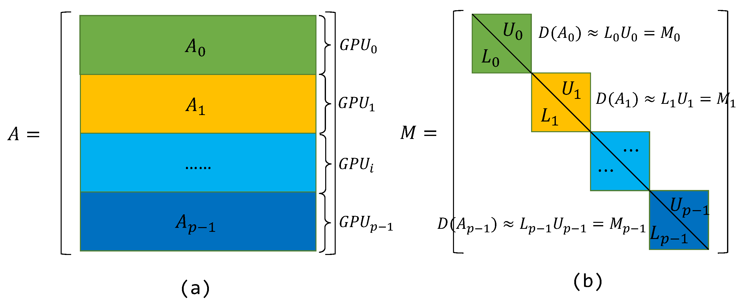
On a distributed system with GPU accelerators, the matrix is always partitioned into sub-matrices each of which is assigned to an accelerator that a process maps to, which is shown in Figure 1a. The popular partitioning strategy is to divide a square matrix in successive rows. A straightforward way to construct M in a distributed system is to conduct incomplete LU factorization (ILU) on the diagonal part of the partitioned matrix residing in each process, which can be expressed as

$$D\left(A_i\right)\approx L_i{U}_i=M_i$$

(4)

where $A_i$ is the partitioned matrix in $i\mathrm{th}$ process, $D\left(A_i\right)$ is the main diagonal part of $A_i$, $L_i$ and $U_i$ is the block lower and upper triangular factors obtained by the ILU factorization, respectively. The process is illustrated in Figure 1b.

$$D\left(A_i\right)\approx L_i{U}_i=M_i$$

(5)

where $A_i$ is the partitioned matrix in $i\mathrm{th}$ process, $D\left(A_i\right)$ is the main diagonal part of $A_i$, $L_i$ and $U_i$ is the block lower and upper triangular factors obtained by the ILU factorization, respectively. The process is illustrated in Figure 1b.

We apply the Block–Jacobi preconditioning method [1], which also can be regarded as the Additive Schwarz Method (ASM) with zero-overlap [25], to perform the preconditioning step as

$$M^{-1}v=\left[\begin{array}{cccc}{\left(M_0\right)}^{-1}& & & \\ & {\left(M_1\right)}^{-1}& & \\ & & \cdots & \\ & & & {\left(M_{p-1}\right)}^{-1}\end{array}\right]\left[\begin{array}{c}{v}_0\\ v_1\\ \cdots \\ v_{p-1}\end{array}\right]=\left[\begin{array}{c}{z}_0\\ z_1\\ \cdots \\ z_{p-1}\end{array}\right]$$

(6)

where $M_i$ is defined as (5), $v_i$ the partitioned vector of a global vector v, $z_i$ is the partitioned vector of the preconditioned vector z, and p is the number of processes or accelerators. The task of the $i\mathrm{th} (0\le i<p)$ process is to compute $z_i$ by solving

$$M_i^{-1}{v}_i=z_i$$

(7)

independently without any communication. The aim of performing ILU factorization in (5) is to form (7) two triangular systems

$$L_i{y}_i=v_i,U_i{z}_i=y_i$$

(8)

which can be solved by forward and backward substitutions.

Equation (8) is hard to parallelize in the ILU preconditioned krylov solvers [24] on parallel architectures because forward and backward substitutions are of inherently sequential feature. Applying ISAI idea [11,17] to (8), we can transform the forward (backward) substitutions into highly parallelized operations consisting of sparse matrix-vector multiplications by computing the inverse of $L_i$ and $U_i$ approximately. In this way, the quality of the preconditioning may degrade and then results in more iterations to converge, but the overall time for the solver could be reduced due to the performance improvement at each preconditioning step. In this work, to seek a balance between performance and exactness, we combine Block–Jacobi preconditioner with Block–ISAI (BJPB-ISAI) in a multi-GPU scenario.

We list BJPB-ISAI method in Algorithm 1. As the GPU workload needs to be launched from hosts, the algorithm runs by a hybrid of Message Passing Interface (MPI) programming model [26] and Compute Unified Development Architecture (CUDA) [27]. MPI is used to launch p host processes each of which is corresponding to a GPU card. Based on the partition strategy illustrated in Figure 1a, the local block triangular factors $L_i$ and $U_i$ can be obtained from the block ILU factorizations on $D\left(A_i\right)$, and they together with a partitioned vector $v_i$ are used as the input parameters. The algorithm outputs the partitioned, preconditioned vector $z_i$ on each GPU. We divide the content of the algorithm into two parts. The first part provides an approximation to the inverses of $L_i$ and $U_i$ requires to be preformed only once during the iterative solver because we consider fixed preconditioners in this work and the ILU factors do not change once the factorization is completed. Specifically, the sparsity pattern estimation for the inverses of $L_i$ and $U_i$, denoted as $L_i^{inv}$ and $U_i^{inv}$, is firstly performed using the symbolic matrix–matrix multiplication on $S\left(\right|L_i\left|\right)$ and $S\left(\right|U_i\left|\right)$ for k times, where $|L_i|$ and $|U_i|$ represent the absolute values of $L_i$ and $U_i$. The sparsity patterns become thicker and with increasing k, but resulting in more memory and computation requirement. The parallel idea of ISAI [17,18] is to solve $L_i^{inv}$ by columns, so we transform $L_i^{inv}$ and $U_i^{inv}$ into BCSC formats for the convenience of accessing row indices in each column of $L_i^{inv}$ or $U_i^{inv}$. More importantly, BCSC formats make the access of $L_i^{inv}$ or $U_i^{inv}$ in the global memory in a coalesced manner. Then two GPU kernels that solve $L_i^{inv}$ and $U_i^{inv}$ in block columns [18] in parallel are launched. The major feature of the GPU algorithm is making full use of the fine-grained programming model of GPU and solves each block column by a warp consisting of 32 consecutive threads (CUDA threads are issued by warps implicitly [28]). The implementation issues are discussed in the next section. Once $L_i^{inv}$ and $U_i^{inv}$ are ready, the second part of Algorithm 1 performs block-based sparse matrix-vector multiplication instead of exactly solving block triangular systems.

Algorithm 1 Block–Jacobi preconditioning with Block–ISAI on multi-GPUs: $M^{-1}v=z$.

Input:  (1) MPI process identifier i; (2) the lower and upper block triangular factors: $L_i$ and $U_i$; (3) the partitioned vector $v_i$; Output:  the preconditioned vector $z_i$;  1: map the $i\mathrm{th}$ process to a GPU with identifier $idev$ on a node;  2: cudaSetDevice($idev$);  3: iffirstcallthen  4:  use $S\left(\right|L_i{|}^k)$ and $S\left(\right|U_i{|}^k)$ to give an estimation of sparsity pattern of the inverses of $L_i$ and $U_i$: $S\left(L_i^{inv}\right)=S\left(\right|L_i{|}^k)$ and $S\left(U_i^{inv}\right)=S\left(\right|U_i{|}^k)$;  5:  transform $L_i^{inv}$ and $U_i^{inv}$ to BCSC format;  6:  // unroll the $for$ loop on GPU to form a warp-based GPU kernel [18]  7:  for $icol=0$ to $m-1$ do  8:   $R_L=$ row indices for $L_i^{inv}(:,icol)$;  9:   locally and temporarily form and solve: $L_i(R_L,R_L)L_i^{inv}(R_L,icol)=I_{icol}^{R_L}$; 10:  end for 11:  // unroll the $for$ loop on GPU to form a warp-based GPU kernel [18] 12:  for $icol=0$ to $m-1$ do 13:   $R_U=$ row indices for $U_i^{inv}(:,icol)$; 14:   locally and temporarily form and solve: $U_i(R_U,R_U)U_i^{inv}(R_U,icol)=I_{col}^{R_U}$; 15:  end for 16:  // transform $L_i^{inv}$ and $U_i^{inv}$ back into BCSR format; 17: end if 18: $y_i=L_i^{inv}{v}_i$; 19: $z_i=U_i^{inv}{y}_i$;

3.2. Multi-GPU Implementation

We implement BJPB-ISAI using open source PETSc (Portable, Extensible Toolkit for Scientific Computation) framework [29] since it offers various, efficient basic vector and matrix operations that reduce the costs of development in scientific applications. Some implementation issues are proposed and discussed in this section.

Most of scientific tools express and store block matrices in scalar formats (usually in CSR formats) by ignoring zero values in blocks. To make our algorithm compatible with user provided matrices in CSR format, we develop a preprocessing procedure using PETSc APIs and cuSPARSE to transform the user provided CSR matrices into PETSc’s BCSR matrices. The pseudo code of the procedure is shown in List 1.

The procedure firstly exploits the subroutines in cuSPARSE [8] to transform a matrix in CSR format into the BCSR format with block size $bs$. The subroutine ($cusparseXcsr2bsrNnz$) estimating the number of non-zero blocks based on a given block size $bs$ is called at first, which is followed by the function $cusparseDcsr2bsr$ to make the real transformation. Once the format transformation is completed, the root process partitions the block matrices by block rows (Figure 1) and sends the partitioned data to each process, while the other processes receive the partitioned data as the data source for the local BCSR matrices. After the communication between the processes is done, each process calls $MatCreateMPIBAIJWithArrays$ from PETSc to construct a parallel block matrix object with its local part. Each process creates a solution vector x and the right hand side b using $VecCreate$ function and only stores the partitioned part locally.

List 1 Procedure for transforming user provided matrices to PETSc’s BCSR matrices.

1: if  $myid==root$ then  2:  cusparseXcsr2bsrNnz($handle$, $dir$, $csrinfo$, ...., $bs$, $bsrinfo$, …, $out:nnzb$);  3:  allocate memory for $browptr$, $bcolval$, $bblkval$ on the device memory  4:  cusparseDcsr2bsr($handle$, $dir$, $csrinfo$, …, $bs$, $bsrinfo$, …);  5:  cudaMemcpy $browptr$, $bcolval$, $bblkval$ back into the host memory  6:  partition the block matrices by block rows (Figure 1a)  7:  for $iproc=1;iproc<p;iproc++$ do  8:   // send the local parts $browpt{r}_{iproc}$, $bcolva{l}_{iproc}$, and $bblkva{l}_{iproc}$ to $iproc$  9:   MPI_Send(…, $to\text{\_}iproc$, …); 10:  end for 11: else 12:  // receive from $root$ as $browpt{r}_{iproc}$, $bcolva{l}_{iproc}$, and $bblkva{l}_{iproc}$ 13:  MPI_Recv(…, $from\text{\_}root$, …); 14: end if 15: MatCreateMPIBAIJWithArrays(…, $bs$, …, $browpt{r}_{iproc}$, $bcolva{l}_{iproc}$, $bblkva{l}_{iproc}$, $\&A$); 16: VecCreate($comm\text{\_}world$, $\&x$); 17: VecCreate($comm\text{\_}world$, $\&b$);

The essence of the Block–Jacobi preconditioner is to use the main diagonal part of the local matrix as the operating matrix for the block ILU factorization locally. Similar to scalar ILU factorizations, PETSc provides full block ILU factorization which can be extracted to form the lower and upper block triangular factors on GPU in Algorithm 1. List 2 shows how the triangular factors be accessed using the low-level data structure in PETSc. The pointer $fact$ to the main data section of the factorization is finally obtained through successive operations from the $subpc$ object. Note that the lower triangular factor is stored in the front part of the arrays in a forward orientation (from top to bottom) without the diagonal blocks (identity matrices), whereas the upper triangular factor is located in the back part of the arrays in a backward orientation (from bottom to top) with the inversed diagonal blocks. The storing strategy is convenient for the subsequent forward and backward substitutions in the preconditioning step if triangular solves are applied to (8). However, instead of using triangular solves in each sub-domain, we aim to employ Block–ISAI where the lower and upper factors are expressed in a general BCSR or BCSC format. Therefore, we rearrange the factors to BCSR format before Algorithm 1 is performed.

List 2 Locally accessing block lower and upper factors.

1: KSPGetPC($ksp$, $\&pc$);  2: PCBJacobiGetSubKSP($pc$, $\&nlocal$, $\&first$, $\&subksp$);  3: KSPGetPC($subksp\left[0\right]$, $\&subpc$);  4: PC_ILU *$ilu$=(PC_ILU *)$subpc$→$data$;  5: Mat $factmat$=((PC_Factor *)$ilu$)→$fact$;  6: Mat_SeqBAIJ * $fact$=(Mat_SeqBAIJ *)$factmat$→data;

The key part of computation on GPU is the numerous small block triangular systems (SBTS) (line 9 and line 14) with a degree of parallelism of m, where m is the number of block rows (columns) for $L_i$ ($U_i$). Different from the large triangular systems in (8), one of the SBTS is viewed as a sub-task for a thread or several threads of a GPU rather than the whole task for a single GPU. How to map the sub-task to threads depends on the algorithmic technique. The SBTS are independent with each other that provides the possibility of exploiting the fine-grained parallelism on the GPU.

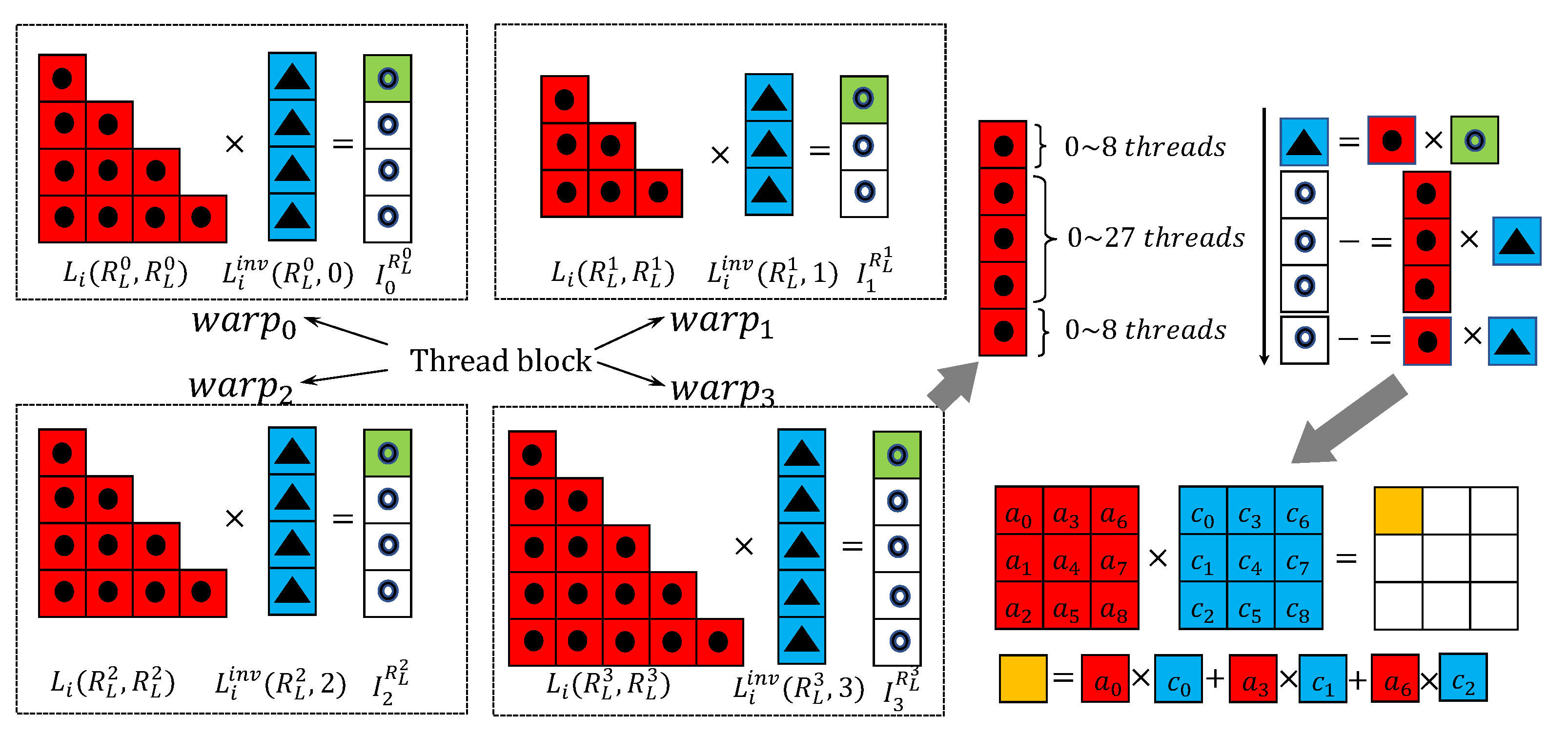
The proposed warp-based algorithm on a single GPU for solving the SBTS [18] is applied to a sub-domain in the multi-GPU case. Figure 2 shows an example of solving the first four block columns of $L_i^{inv}$ using a thread block containing 128 threads. From the hardware point of view, the basic unit of execution and dispatching on a streaming multiprocessor (SM) of the GPU are warps and a warp groups 32 consecutive threads that are executed in Single Instruction Multiple Thread (SIMT) model. Therefore, the threads in the thread block are divided into 4 warps each of which is implicitly issued by the warp scheduler on the GPU. A total of 32 threads in a warp solve one of the four SBTS with executing exactly the same instruction but accessing different data. The right part of Figure 2 illustrates the process of solving a $5\times 5$ lower triangular system with block size 3 in $war{p}_3$. To explain how the $5\times 5$ lower triangular system is solved by $war{p}_3$, we simply denote the system as

$$WSol=rhs$$

(9)

where $W=L_i(R_L^3,R_L^3)$, $Sol=L_i^{inv}(R_L,3)$, and $rhs=I_3^{R_L^3}$. The solution ($Sol$, marked in black triangles in blue squares) is solved by looping over five block columns. In the process of handing the first block column for example, three steps are required. The first step uses the first nine threads in the warp to cover $W(1,1)$, and make a block–block multiplication to get $Sol\left(1\right)$. Once $Sol\left(1\right)$ is obtained, the following two steps use $Sol\left(1\right)$, $W(2,1)$, $W(3,1)$, $W(4,1)$ and $W(5,1)$ to update $rhs\left(2\right)$, $rhs\left(3\right)$, $rhs\left(4\right)$ and $rhs\left(5\right)$ by

$$rhs\left(k\right)=rhs\left(k\right)-W(k,1)\times Sol\left(1\right)(k=2,3,4,5)$$

Because 32 threads in the warp can only cover three complete $3\times 3$ blocks, the updates of $rhs\left(2\right)$, $rhs\left(3\right)$, and $rhs\left(4\right)$ are performed by the first 27 threads in the same round whereas the update of $rhs\left(5\right)$ is performed by the first nine threads in the next round. Then the warp handles the second block column as it does for the first one. $sol\left(2\right)$ is first obtained by $Sol\left(2\right)=inv\left(W\right(2,2\left)\right)\times rhs\left(2\right)$. Once $Sol\left(2\right)$ is obtained, it is used to accumulate $rhs\left(3\right)$, $rhs\left(4\right)$ and $rhs\left(5\right)$. The process will go on for the third, fourth, fifth block columns until $Sol\left(3\right)$, $Sol\left(4\right)$ and $Sol\left(5\right)$ are obtained.

Different from the scalar versions [17], all computations are performed blockwise. For example, the lower right corner of Figure 2 shows the fine-grained block–block multiplication where each thread computes only one element for the resulting block by looping over one row of the first block and one column of the second block. So computing the multiplication of two $3\times 3$ blocks requires nine threads, and 32 threads in a warp can accumulate three blocks in $rhs$ simultaneously. The low-latency, programmable, on-chip shared memory provides a communication channel for threads within a thread block. In the implementation, the current solution (marked in triangles in blue squares) is stored in the shared memory for data sharing between different threads and this data storage strategy also leads to performance improvement because accessing data from the shared memory is much faster than accessing from the global memory.

4. Experiments

4.1. Experiment Setup

We used four Tesla K20 and Tesla V100 GPUs to conduct experiments and make comparisons for the proposed BJPB-ISAI algorithm in this section. A comparison of the main parameters of the two generations of NVIDIA’s GPUs are shown in

Table 2. A comparison of the main parameters of Tesla K20 and Tesla V100 GPUs.

Tesla Product	Tesla K20	Tesla V100
GPU	GK110	GV100
Core Clock	706 MHz	1530 MHz
Stream Processors	2496	5120
Memory Interface	320-bit DDR5	4096-bit HBM2
Memory size	5 GB	16 GB
Peak FP32 TFLOPS	3.52	15.7
Peak FP64 TFLOPS	1.17	7.8
Shared Memory size	16/32/48 KB	configurable up to 96 KB
Register File Size/SM	256 KB	256 KB

. Compared to Tesla K20, Tesla V100 delivered major performance improvements and had nearly 6.7 times higher double precision floating-point peak performance.

The host of a Tesla K20 GPU node, with CentOS 6.4 installed, was configured with Intel E5-2680 V2 CPUs having a clock rate of 2.8 GHz and a memory size of 128 GB (host-1), while the host of a Tesla V100 GPU node, with CentOS 7.5 installed, was configured with E5-2640 V4 CPUs having a clock rate of 2.4 GHz and a memory size of 128 GB (host-2). PETSc-3.10.2, CUDA-aware OpenMPI v3.1.4 [30] and CUDA 6.5.14 [31] were used on the K20 GPU cluster, while PETSc-3.14, OpenMPI-4.0 [26] and CUDA 10.0 [27] were employed on the V100 GPU cluster. The CUDA drivers for K20 and V100 GPUs were 340.29 and 440.64, respectively. The multi-GPU version of GMRES algorithm was developed and integrated into PETSc, so the two environments shared exactly the same codes except the shared libraries including cuSPARSE and MPI even though the PETSc version was different. On both clusters, PETSc was installed without the debugging option that is used as the reference for analyzing speedups. For all the linear systems solved in the test cases, the right-preconditioned GMRES with restart 30 was employed. All floating-point operations on CPUs and GPUs were performed in double precision.

4.2. Results

We used the matrix atmosmodd from SuiteSparse Matrix Collection [32] as the first test case. The matrix in CSR format had 1,270,432 rows (columns) and 8,814,880 non-zeros. The procedure in List 1 transformed the matrix to BCSR format using a block size of 4, and the resulting matrix consisting of 317,608 block rows (columns) and 2,190,844 non-zero blocks was solved by GMRES(30) with BJPB-ISAI and a relative tolerance of ${10}^{-8}$.

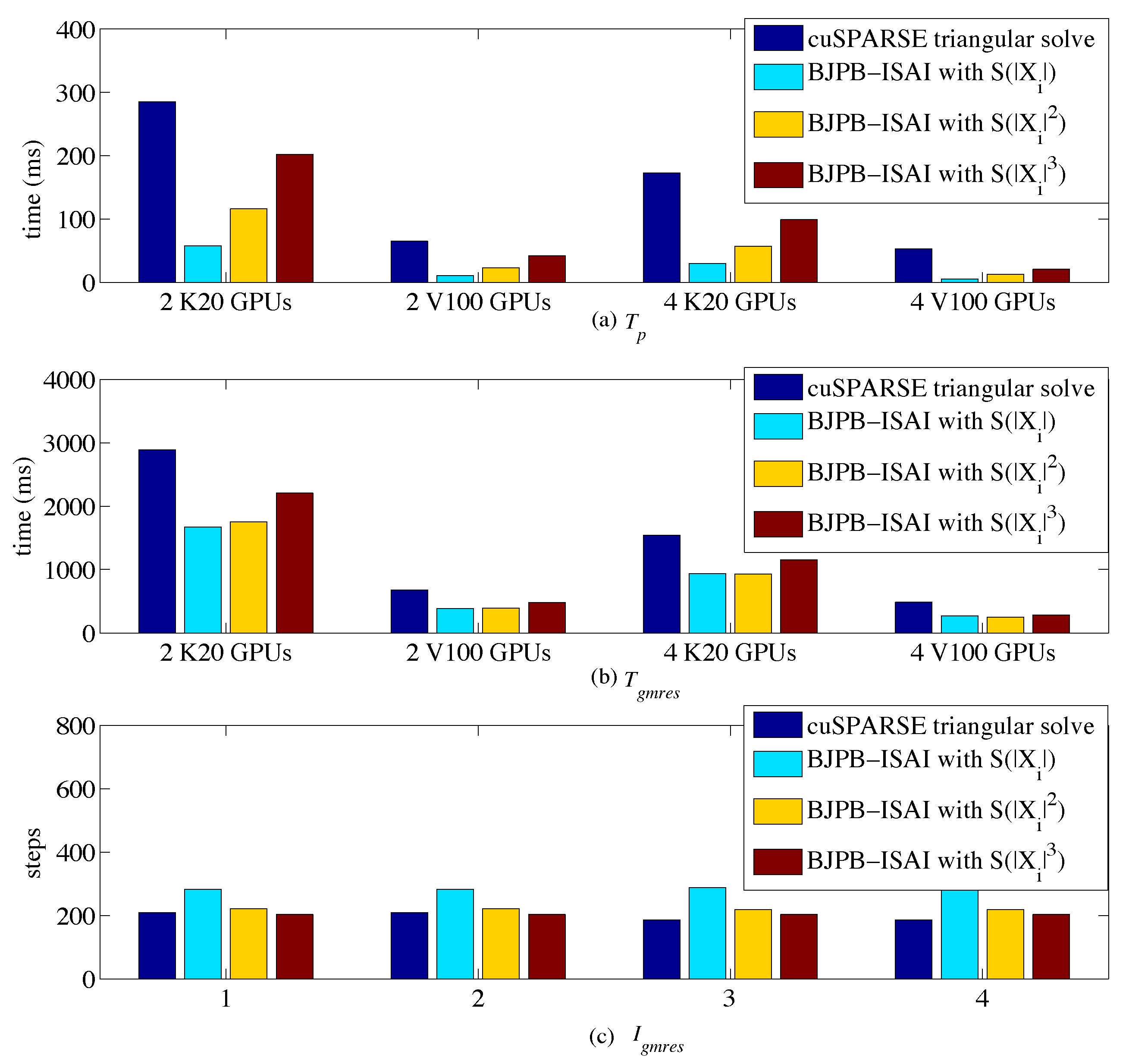
Figure 3 shows the performance results on up to four Tesla K20 and V100 GPUs respectively in terms of $T_p$, $T_{gmres}$, and $I_{gmres}$, where $T_p$ is the wall clock time for computing 30 preconditioning steps (i.e., (7)), $T_{gmres}$ represents the total wall clock time for GMRES(30) to converge, and $I_{gmres}$ is the total number of iterations for GMRES(30).

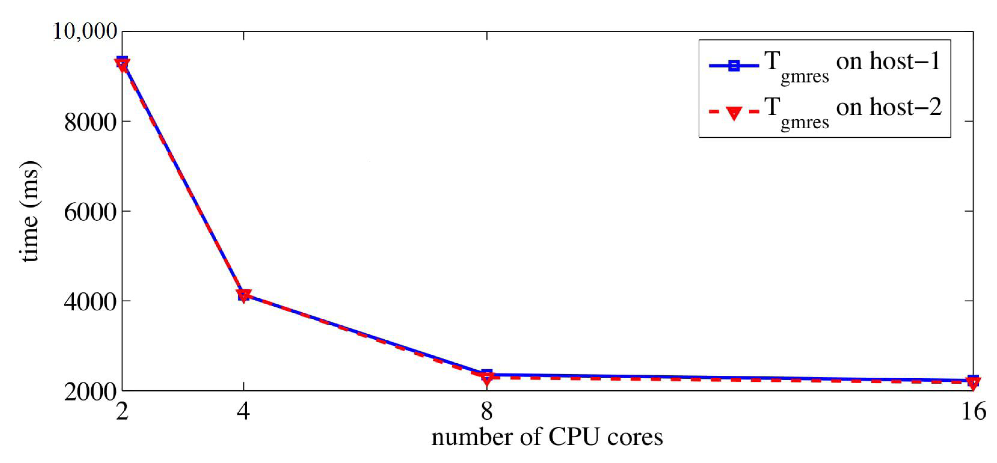
To make a performance comparison between CPU and GPU results, we show $T_{gmres}$ on CPUs in Figure 4. It is reported in [7] that the level-scheduling based triangular solve successfully gained speedups on the atmosmodd case. By comparing $T_{gmres}$ in Figure 4 to $T_{gmres}$ obtained by block triangular solves from cuSPARSE library in Figure 3, we also observed an advantage of GPU block triangular solves over the CPU counterpart. When four GPUs were used, preconditioned GMRES using cuSPARSE’s block triangular solves could achieve $4.6\times$ and $1.44\times$ speedups on Tesla V100 and Tesla K20 GPU platforms over the pure CPU preconditioned GMRES on 16 cores.

Then we looked at the results from BJPB-ISAI($|X_i{|}^k$) ($k\le 3$) and observed that $I_{gmres}$ decreased with increasing the density of the sparsity pattern for $L_i^{inv}$ and $U_i^{inv}$. This is expected because the denser sparsity for $L_i^{inv}$ and $U_i^{inv}$ made the approximate inverses close to the exact ones. The penalty of increasing the sparsity densities of $L_i^{inv}$ and $U_i^{inv}$ was that it not only made the overhead of doing preconditioning increase but also made the wall clock times of solving $L_i^{inv}$ and $U_i^{inv}$ increase. To measure the real wall clock times for GMRES with BJPB-ISAI algorithm, we included both $T_{gmres}$ and the overhead of gaining $L_i^{inv}$ and $U_i^{inv}$ as

$$T_{total}=T_{gmres}+T_{BISAI}$$

(10)

where $T_{BISAI}$ is the time used to gain $L_i^{inv}$ and $U_i^{inv}$. Figure 5 shows a comparison of $T_{BISAI}$ on Tesla K20 and V100. Note that $T_{BISAI}$ was measured as the maximum value among the used GPUs because there might be imbalanced workload when multiple GPUs were employed. We divided $T_{BISAI}$ into $T_{ESP}$, $T_{SBTS}$ and $T_{csr2csc}$ where $T_{ESP}$ is the time used for estimating the sparsity pattern (ESP) of $|L_i{|}^k$ and $|U_i{|}^k$, $T_{SBTS}$ is the time used for solving the SBTS, and $T_{csr2csc}$ is the time used for format transformation in Algorithm 1. We observe from Figure 5b that solving SBTS achieved over $9\times$ speedup on Tesla V100 GPU compared to Tesla K20 GPU, and it shows nearly linear scalability up to four GPUs. The scalability is expected, because each warp independently solved a small block triangular system without any data dependency on other warps, which made maximum use of the fine-grained feature of GPUs. On K20 GPUs, because the L1 cache was not used for global memory loads but only for register spills to local memory [28], we preferred a configuration of 48 KB shared memory and 16 KB L1 cache to guarantee that there were enough shared memory spaces for storing temporary variables whose sizes varied with block sizes. According to NVIDIA’s profiler, the achieved_occupancy for warps was about 90% on Tesla V100 GPUs, whereas it was 73% on Tesla K20 GPUs. This is because warps had overlap with loading data from the global memory, and using L1 cache on Tesla V100 with low-latency was effective for latency hiding. $T_{ESP}$ and $T_{csr2csc}$ implemented using cuSPARSE library were much reduced due to the performance improvement in both GPU hardware and the software library.

Figure 3b shows the BJPB-ISAI implementation had an advantage over the cuSPARSE implementation on both K20 and V100 GPUs in terms of $T_{gmres}$. By counting $T_{BISAI}$ for BJPB-ISAI algorithm, we still observed GMRES(30) with BJPB-ISAI($|X_i|$) could achieve 1.6x over that with cuSPARSE on Tesla K20 platform and GMRES(30) with BJPB-ISAI $\left(\right|X_i{|}^2$) using four V100 GPUs could achieve 1.87x over that with cuSPARSE on Tesla V100 platform.

In the second case, we solved a non-linear system from the 2D nonlinear driven cavity problem expressed as

$$\begin{array}{ccc}\hfill -▵u-\frac{\partial \omega }{\partial y}& =& 0,\hfill \\ \hfill -▵v-\frac{\partial \omega }{\partial x}& =& 0,\hfill \\ \hfill -▵\omega +u\frac{\partial \omega }{\partial x}+v\frac{\partial \omega }{\partial y}& =& 0.\hfill \end{array}$$

For the velocity variables $(u,v)$, the no-slip, rigid-wall Dirichlet conditions were applied. For vorticity $\omega$, the boundary condition is given by $\omega =-\frac{\partial u}{\partial x}+\frac{\partial v}{\partial y}$. The Reynolds number was set to 1 in this case. The problem was solved on a $600\times 600$ mesh in a unit square domain by using a five-point stencil finite difference method. Since each mesh cell was associated with three variables, the resulting linear system at each Newton step was formed by the Jacobian matrix with a block size of three. The relative tolerance for each linear system was set to ${10}^{-5}$. The convergence criteria was set to ${10}^{-8}$ for the non-linear process. In each subdomain, the block ILU(0) factorization was employed. We note that the linear system could not converge without using the ILU preconditioner.

The non-linear system required three Newton steps to converge to the given tolerance. At each Newton step, a linear system consisting of 1,080,000 block rows (columns) and 1,797,600 non-zero blocks needed to be solved. The sparsity pattern for the linear system stayed unchanged at different Newton steps, therefore the data dependency and computational workload for the preconditioning step was also unchanged even though the data in the linear system changed at every Newton step.

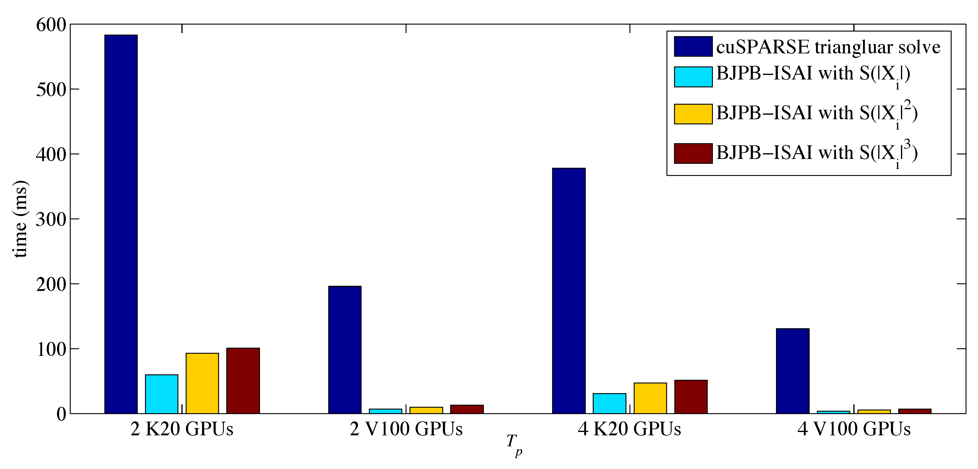
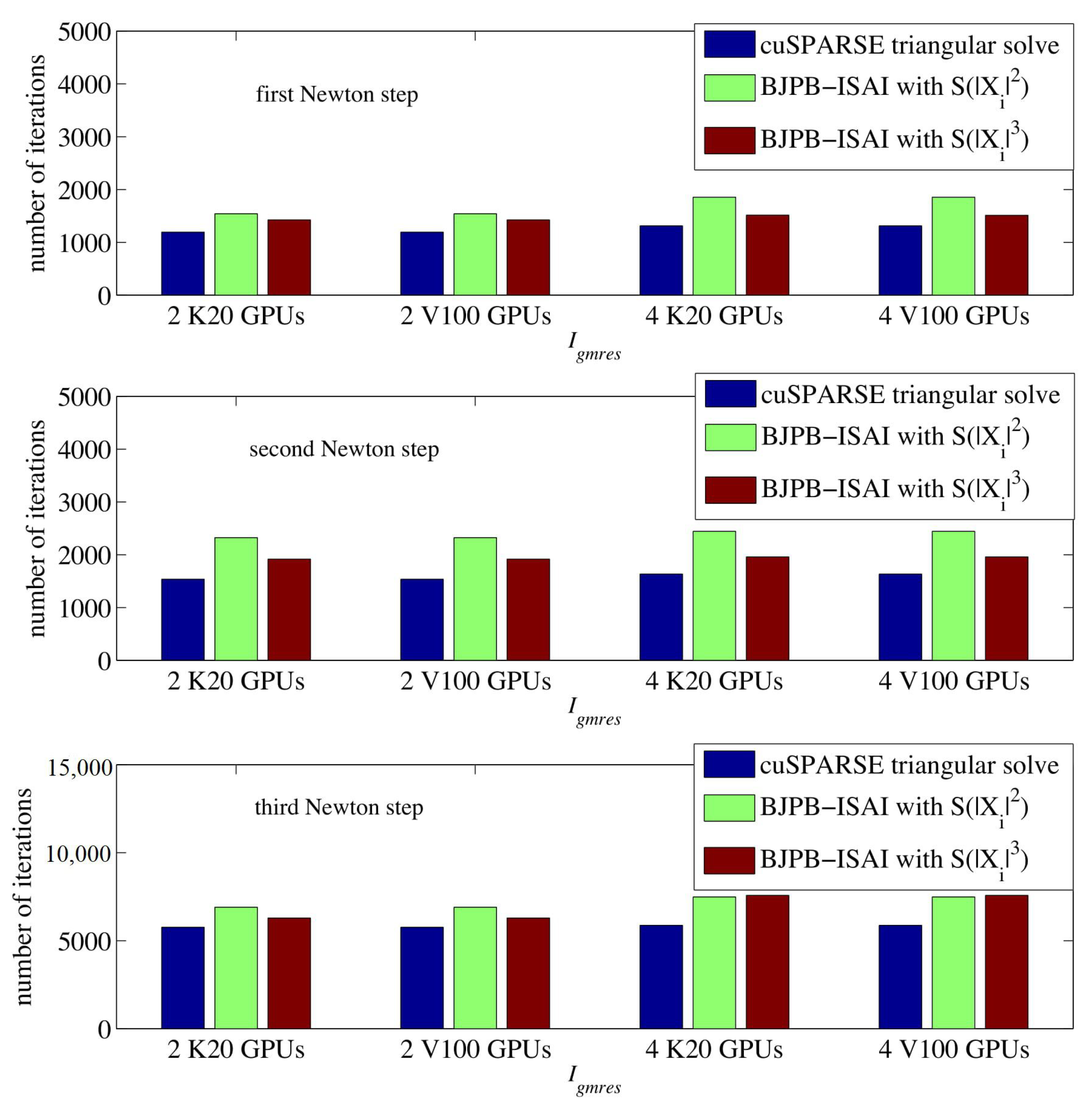
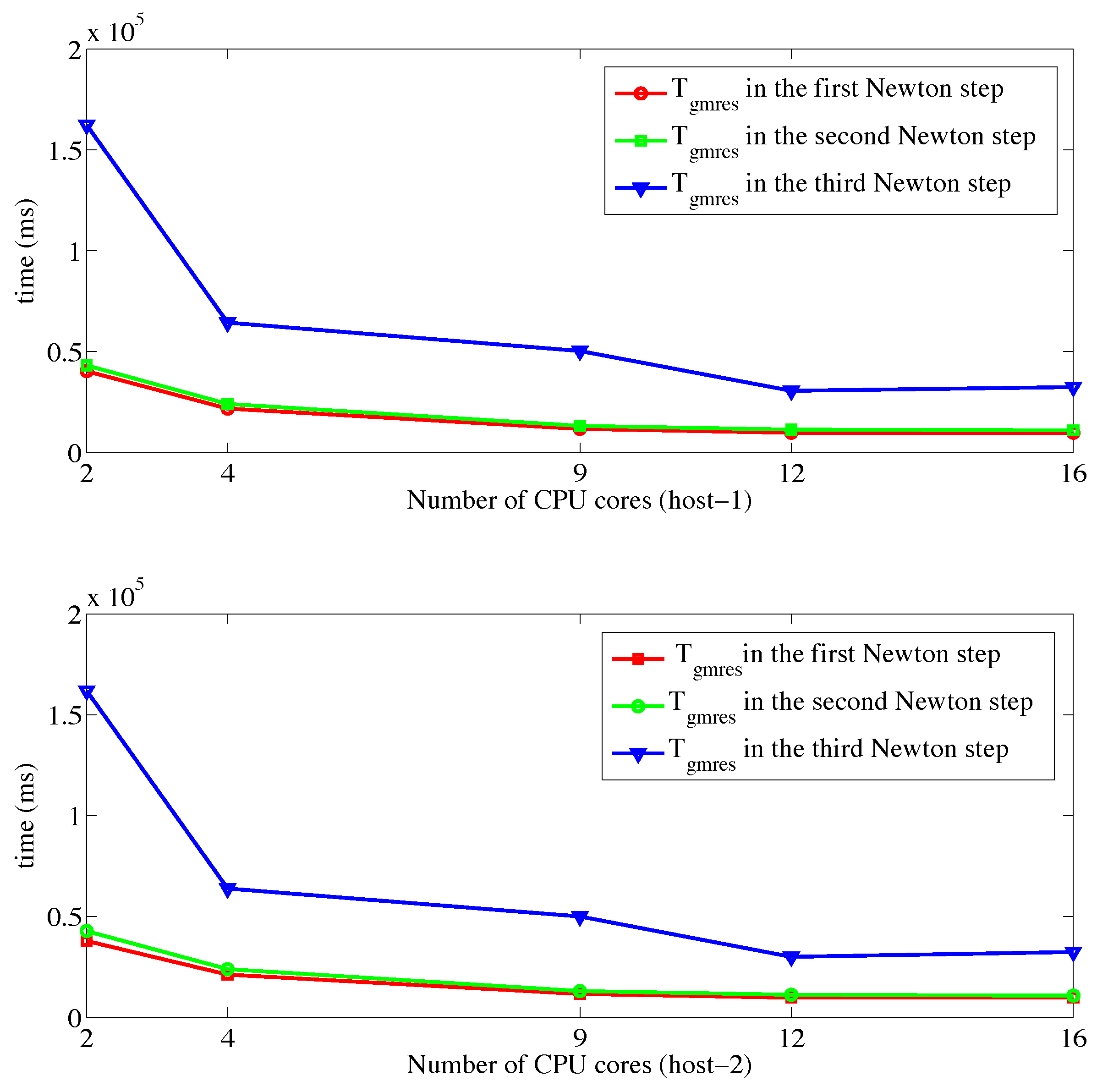
Figure 6 shows a comparison of $T_p$ between Tesla K20 and Tesla V100 GPUs. Figure 7 and Figure 8 show the comparisons of $T_{gmres}$ and $I_{gmres}$ in each Newton step, respectively. Because the sparsity pattern of the matrix generated by the five-point finite different stencil had a strong data dependence using the level-scheduling algorithm for triangular solves, it became the bottleneck of the whole preconditioned GMRES on GPUs. On Tesla K20 GPUs, $T_p$ using cuSPARSE library’s block triangular solved accounts for over 80% of the average cost of 30 GMRES steps (i.e., $30\times \frac{T_{gmres}}{I_{gmres}}$). Due to the poor performance of the preconditioning step on GPUs, we did not observe obvious performance improvement when comparing $T_{gmres}$ to that on the CPU platform which is shown in Figure 9. On Tesla V100 GPUs, the performance of the triangular solves using cuSPARSE 10.0 was much improved compared to Tesla K20 GPU. The sparsity pattern of the matrix had very strong data dependency that made the concurrency of the triangular solve low using the level-scheduling algorithm, so we attributed the performance improvement for cuSPARSE to the faster and more efficient memory on Tesla V100 GPUs. However, $T_p$ on four GPUs was nearly the same as that on CPUs, which means the speedups was obtained only by the block sparse matrix–vector multiplication (block-SpMV) and vector operations in GMRES.

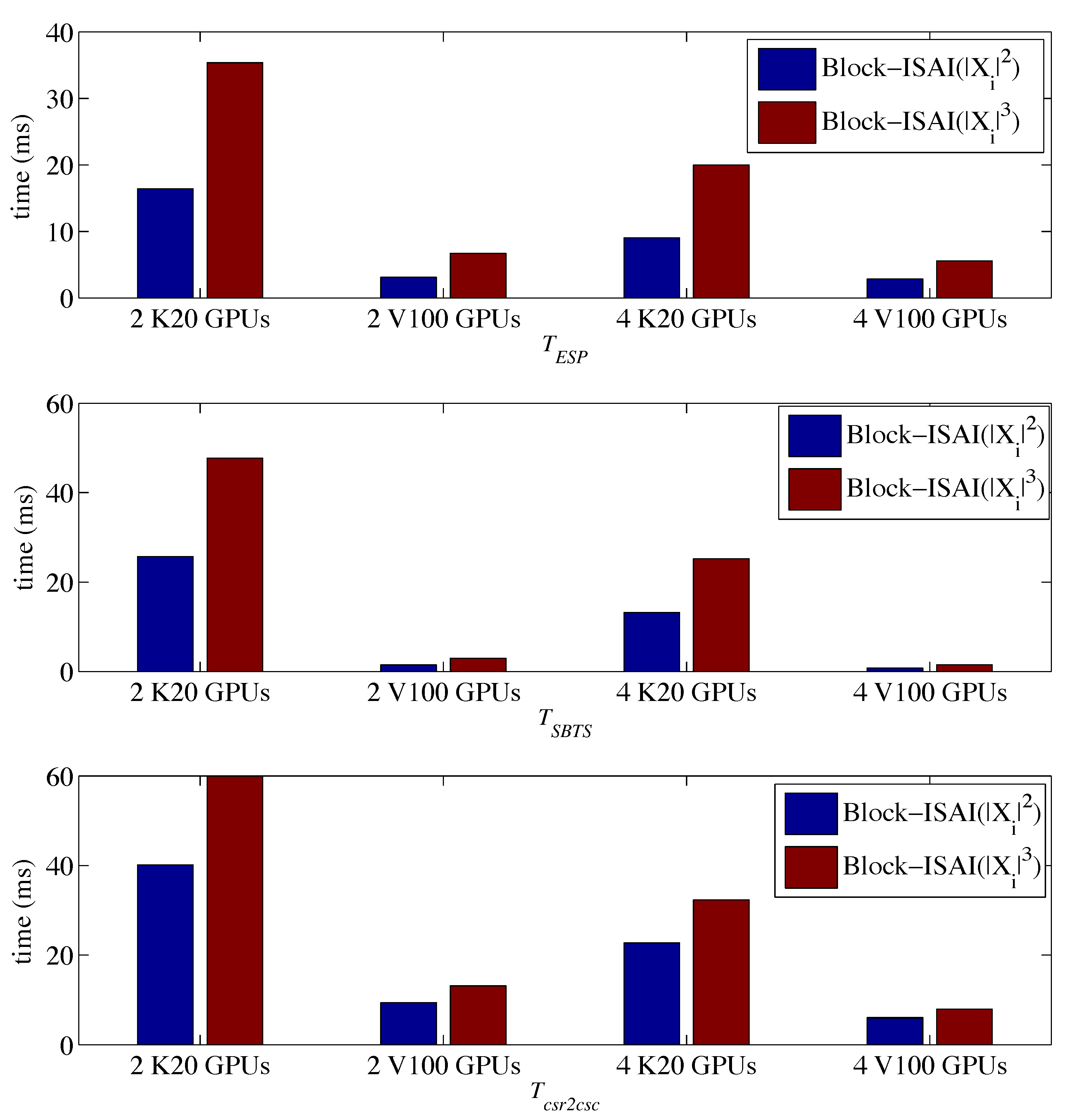
By using BJPB-ISAI, we see from Figure 7 and Figure 8 that both $T_p$ and $T_{gmres}$ was much reduced. Note that $T_{gmres}$ from BJPB-ISAI with $S\left(\right|X_i\left|\right)$ is not reported in Figure 7 because the preconditioner constructed by $S\left(\right|X_i\left|\right)$ was not accurate enough for GMRES(30) in the third Newton step to converge within 10,000 iterations. For BJPB-ISAI($|X_i{|}^2$) and BJPB-ISAI($|X_i{|}^3$), the preconditioners were effective enough to make GMRES converge even though they resulted in more GMRES iterations than the exact preconditioner from cuSPARSE. With increasing the density of the sparsity pattern, $I_{gmres}$ gradually reduced, and BJPB-ISAI($|X_i{|}^3$) was close to the preconditioning using exact block triangular solves in terms of $I_{gmres}$. Before calculating the speedup on Tesla V100 over Tesla K20, we show a comparison of $T_{BISAI}$ in Figure 10. Since there were three different linear systems that needed to be solved in this non-linear process, Block–ISAI for inverse approximations was executed three times, and Figure 10 reports the average values from these observations.

Compared to $T_{gmres}$ shown in Figure 7, $T_{BISAI}$ is only a tiny part of $T_{total}$ in (10). Compared to Block–ISAI($|X_i{|}^2$), Block–ISAI($|X_i{|}^3$) results in smaller values of $T_{total}$ for all three linear systems, and an average of 3.3x and 5.1x speedups can be obtained for the three linear systems on Tesla K20 and Tesla V100 over the corresponding block triangular solves using cuSPARSE.

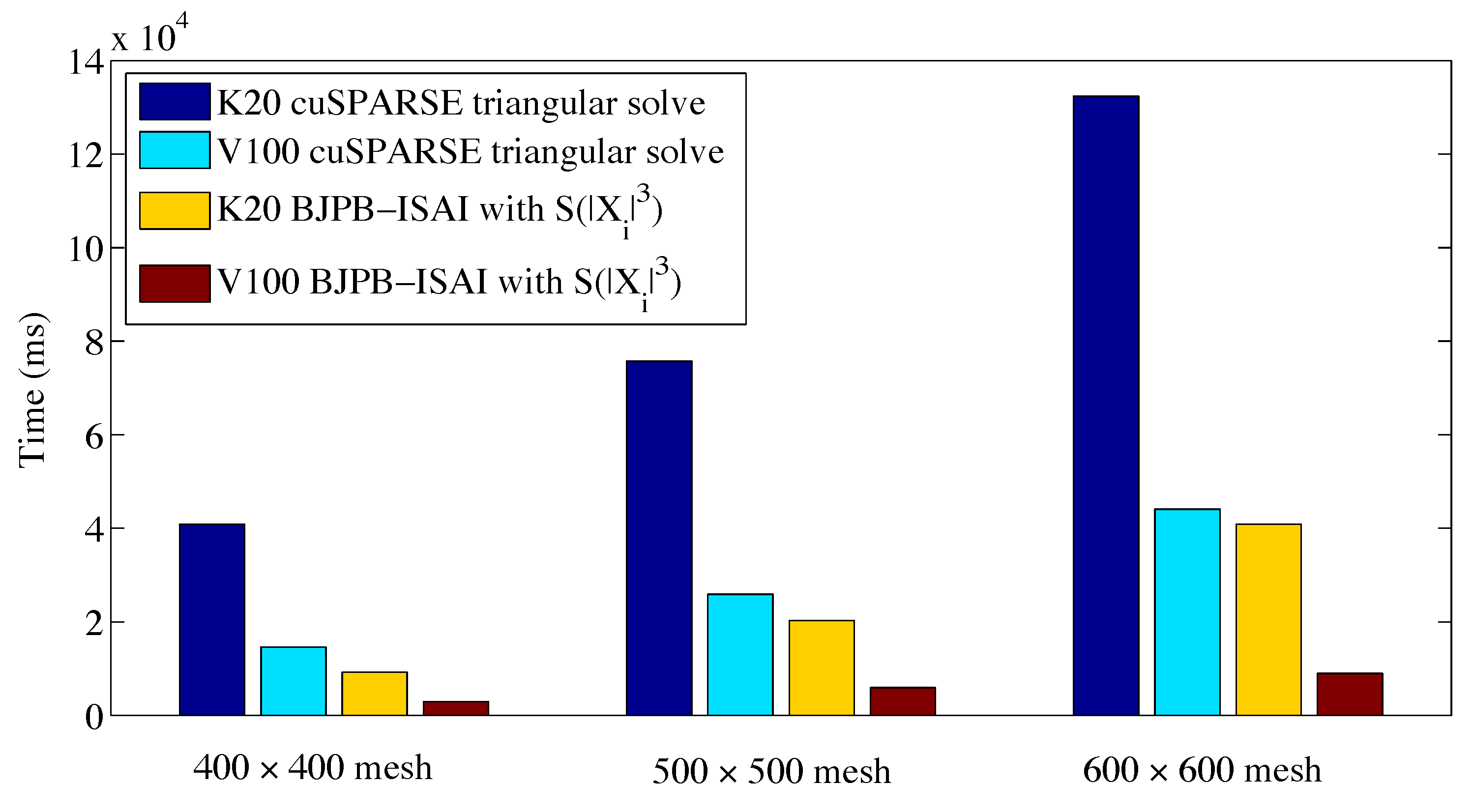
Using BJPB-ISAI($|X_i{|}^3$) and cuSPARSE’s triangular solves for preconditioning on four GPUs, in Figure 11, we report the comparisons of the overall time for solving the non-linear problem with increasing mesh size from $400\times 400$ to $600\times 600$. The number of non-zero blocks for the matrices from the three mesh configurations are 798,400, 1,248,000, 1,797,600, respectively. We observe that in each configuration, the overall cost obtained by BJPB-ISAI($|X_i{|}^3$) was smaller than that obtained by cuSPARSE’s triangular solves, which indicates that BJPB-ISAI($|X_i{|}^3$) was a stable and effective preconditioner for this problem.

5. Conclusions

In this work, the block version of ISAI (B-ISAI)is studied on multiple GPUs as a sub-domain constructor for the inverses of ILU factors in the Block–Jacobi preconditioning technique. The algorithm is integrated in the open source PETSc framework. The two experiments from the real problems with the block matrix show that BJPB-ISAI algorithm offers a better preconditioner than the parallel level-scheduling based preconditioning in terms of total computing time of GMRES(30), but at the sacrifice of the number of GMRES iterations. It is found that in the extreme cases where strong data dependency exists (for example, block matrices from the five-point finite difference method), the performance of a linear solver using BJPB-ISAI can be much improved on GPUs than that using block triangular solves from the cuSPARSE library. The comparisons on two generations of Tesla GPUs are conducted, compared to Tesla K20 GPU, the Tesla V100 GPU shows great performance improvement on the essential steps of the proposed PBJB-ISAI preconditioner.

References

- Saad, Y. Iterative Methods for Sparse Linear Systems, 2nd ed.; Society for Industrial and Applied Mathematics: Philadelphia, PL, USA, 2003. [Google Scholar]
- Naumov, M. Parallel Solution of Sparse Triangular Linear Systems in the Preconditioned Iterative Methods on the GPU. Available online: https://research.nvidia.com/sites/default/files/pubs/2011-06_Parallel-Solution-of/nvr-2011-001.pdf (accessed on 29 June 2021).
- Compute Unified Device Architecture. Available online: https://developer.nvidia.com/cuda-toolkit (accessed on 20 April 2021).
- Anzt, H.; Sawyer, W.; Tomov, S.; Luszczek, P.; Dongarra, J. Optimizing Krylov Subspace Solvers on Graphics Processing Units. In Proceedings of the 2014 IEEE 28th International Parallel & Distributed Processing Symposium Workshops, Phoenix, AZ, USA, 19–23 May 2014; pp. 941–949. [Google Scholar]
- Clark, M.A.; Strelchenko, A.; Vaquero, A.; Wagner, M.; Weinberg, E. Pushing Memory Bandwidth Limitations Through Efficient Implementations of Block-Krylov Space Solvers on GPUs. Comput. Phys. Commun. 2018, 233, 29–40. [Google Scholar] [CrossRef] [Green Version]
- Rupp, K.; Tillet, P.; Rudolf, F.; Weinbub, J.; Selberherr, S. ViennaCL-Linear Algebra Library for Multi - and Many-Core Architectures. SIAM J. Sci. Comput. 2016, 38, S412–S439. [Google Scholar] [CrossRef] [Green Version]
- Li, R.P.; Saad, Y. GPU-accelerated preconditioned iterative linear solvers. J. Supercomput. 2013, 63, 443–466. [Google Scholar] [CrossRef]
- CUDA Toolkit Documentation for cuSPARSE. Available online: https://docs.nvidia.com/cuda/cusparse/ (accessed on 5 April 2021).
- Liu, W.; Li, A.; Hogg, J.; Duff, I.S.; Vinter, B.A. Synchronization-Free Algorithm for Parallel Sparse Triangular Solves. Lect. Notes Comput. Sci. 2016, 9833, 617–630. [Google Scholar]
- Liu, W.; Li, A.; Hogg, J.D.; Duff, I.S.; Vinter, B.A. Fast synchronization-free algorithms for parallel sparse triangular solves with multiple right-hand sides. Concurrency Comput. Prac. Exp. 2017, 29, e4244. [Google Scholar] [CrossRef]
- Kashi, A.; Nadarajah, S. Fine-grain parallel smoothing by asynchronous iterations and incomplete sparse approximate inverses for computational fluid dynamics. In Proceedings of the AIAA Scitech 2020 Forum, Orlando, FL, USA, 6–10 January 2020. [Google Scholar]
- Chow, E.; Patel, A. Fine-grained parallel incomplete LU factorization. SIAM J. Sci. Comput. 2015, 37, C169–C193. [Google Scholar] [CrossRef]
- Chow, E.; Anzt, H.; Dongarra, J. Asynchronous Iterative Algorithm for Computing Incomplete Factorizations on GPUs. Lect. Notes Comput. Sci. 2015, 9137, 1–16. [Google Scholar]
- Dessole, M.; Marcuzzi, F. Fully iterative ILU preconditioning of the unsteady Navier-Stokes equations for GPGPU. Comput. Math. Appl. 2019, 77, 907–927. [Google Scholar] [CrossRef]
- Anzt, H.; Chow, E.; Dongarra, J. Iterative Sparse Triangular Solves for Preconditioning. Lect. Notes Comput. Sci. 2015, 9233, 650–661. [Google Scholar]
- Anzt, H.; Chow, E.; Szyld, D.B.; Dongarra, J. Domain Overlap for Iterative Sparse Triangular Solves on GPUs. In Software for Exascale Computing- SPPEXA 2013–2015; Springer: Cham, Switzerland, 2016; pp. 527–545. [Google Scholar]
- Anzt, H.; Huckle, T.K.; Bräckle, J.; Dongarra, J. Incomplete Sparse Approximate Inverses for Parallel Preconditioning. Parallel Comput. 2018, 71, 1–22. [Google Scholar] [CrossRef]
- Ma, W.P.; Hu, Y.W.; Yuan, W.; Liu, X.Z. GPU Preconditioning for Block Linear Systems Using Block Incomplete Sparse Approximate Inverses. Math. Probl. Eng. 2021, 2021, 5558508. [Google Scholar] [CrossRef]
- Kolotilina, L.Y.; Yeremin, A.Y. Factorized Sparse Approximate Inverse Preconditionings I. Theory. SIAM J. Matrix Anal. Appl. 1993, 14, 45–58. [Google Scholar] [CrossRef]
- Duin, V.; Arno, C.N. Scalable Parallel Preconditioning with the Sparse Approximate Inverse of Triangular Matrices. SIAM J. Matrix Anal. Appl. 1999, 20, 987–1006. [Google Scholar] [CrossRef] [Green Version]
- Bertaccini, D.; Filippone, S. Sparse approximate inverse preconditioners on high performance GPU platforms. Comput. Math. Appl. 2016, 71, 693–711. [Google Scholar] [CrossRef] [Green Version]
- He, G.; Yin, R.; Gao, J. An efficient sparse approximate inverse preconditioning algorithm on GPU. Concurr. Comput. Pract. Exper. 2019, 32. [Google Scholar] [CrossRef]
- Gao, J.; Chen, Q.; He, G. A thread-adaptive sparse approximate inverse preconditioning algorithm on multi-GPUs. Parallel Comput. 2021, 101, 102724. [Google Scholar] [CrossRef]
- Saad, Y.; Schultz, M.H. GMRES: A Generalized Minimal Residual Algorithm for Solving Nonsymmetric Linear Systems. SIAM J. Sci. Stat. Comput. 1986, 7, 856–869. [Google Scholar] [CrossRef] [Green Version]
- Cai, X.C.; Saad, Y. Overlapping Domain Decomposition Algorithms For General Sparse Matrices. Numer. Linear. Algebr. 1994, 3, 221–237. [Google Scholar] [CrossRef]
- OpenMPI v4.0 Series. Available online: https://www.open-mpi.org/doc/current (accessed on 24 March 2021).
- CUDA Toolkit Documentation v10.0.130. Available online: https://docs.nvidia.com/cuda/archive/10.0/ (accessed on 5 April 2021).
- Cheng, J.; Grossman, M.; McKercher, T. Professional CUDA C Programming; Wiley: Hoboken, NJ, USA, 2014. [Google Scholar]
- Balay, S.; Abhyankar, S. PETSc Web Page. Available online: https://www.mcs.anl.gov/PETSc (accessed on 30 April 2021).
- OpenMPI v3.1 Series. Available online: https://www.open-mpi.org/doc/v3.1/ (accessed on 24 March 2021).
- CUDA 6.5 Production Release. Available online: https://developer.nvidia.com/cuda-toolkit-65 (accessed on 5 April 2021).
- Davis, T.; Hu, Y. The University of Florida Sparse Matrix Collection. ACM T. Math. Software 2011, 38, 1–25. [Google Scholar] [CrossRef]
Figure 1.
Matrix partition and the process of constructing preconditioners.
Figure 2.
Illustration of warp-based algorithm for solving SBTS on each GPU. Each warp extracts a sub-matrix from using the block-row indices of the block-column of . Then the block-column of , i.e., is solved by the warp independently.
Figure 3.
Atmosmodd case: comparisons between cuSPARSE triangular solve-based preconditioning and BJPB-ISAI with three sparsity levels for L’s and U’s inverses. (a) : wall clock times for computing 30 preconditioning steps. (b) : total wall clock time for computing GMRES(30) to converge. (c) : the total number of iterations used for GMRES(30) to converge.
Figure 4.
Atmosmodd case: on host-1 and host-2.
Figure 5.
Atmosmodd case: overhead breakdown of gaining and using Block–ISAI with , and . (a) : time used for estimating the sparsity pattern. (b) : time used for solving small block triangular systems. (c) : time used for format transformations.
Figure 6.
Driven cavity case: comparisons of between Tesla K20 GPUs and Tesla V100 GPUs. denotes the wall clock times for performing 30 preconditioning steps.
Figure 7.
Driven cavity case: comparisons of between Tesla K20 GPUs and Tesla V100 GPUs. denotes the wall clock times for running GMRES(30) to converge in each Newton step.
Figure 8.
Driven cavity case: comparisons of between Tesla K20 GPUs and Tesla V100 GPUs. denotes the total number of iterations used for GMRES(30) in each Newton step.
Figure 9.
Driven cavity case: on host-1 and host-2 for all three linear systems.
Figure 10.
Driven cavity case: overhead breakdown of gaining and using Block–ISAI with and . (top) : time used for estimating the sparsity pattern. (middle) : time used for solving small block triangular systems. (bottom) : time used for format transformations.
Figure 11.
Driven cavity case: the comparisons of overall times with increasing mesh sizes of the problem.