
Energy Management of a Multi-Source Power System


1
Engineering Systems Management Program, American University of Sharjah, Sharjah 26666, United Arab Emirates
2
Department of Industrial Engineering, American University of Sharjah, Sharjah 26666, United Arab Emirates
3
Department of Electrical Engineering, American University of Sharjah, Sharjah 26666, United Arab Emirates
*
Authors to whom correspondence should be addressed.
Algorithms 2021, 14(7), 206; https://0-doi-org.brum.beds.ac.uk/10.3390/a14070206
Submission received: 5 May 2021
/
Revised: 6 July 2021
/
Accepted: 6 July 2021
/
Published: 7 July 2021
(This article belongs to the Special Issue Scheduling: Algorithms and Applications)
Abstract
:This work focuses on energy management for a system operated by multiple energy sources which include batteries, super capacitors, a hydrogen fuel cell, and a photovoltaic cell. The overall objective is to minimize the power consumption from all sources needed to satisfy the system’s power demand by optimizing the switching between the different energy sources. A dynamic mathematical model representing the energy sources is developed taking into account the different constraints on the system, i.e., primarily the state-of-charge of the battery and the super capacitors. In addition to the model, a heuristic approach is developed and compared with the mathematical model. Both approaches were tested on a multi-energy source ground robot as a prototype. The novelty of this work is that the scheduling of an energy system consisting of four different types of sources is compared by performing analysis via dynamic programming, and a heuristic approach. The results generated using both methods are analyzed and compared to a standard mode of operation. The comparison validated that the proposed approaches minimize the average power consumption across all sources. The dynamic modeling approach performs well in terms of optimization and provided a superior switching sequence, while the heuristic approach offers the definite advantages in terms of ease of implementation and simple computation requirements. Additionally, the switching sequence provided by the dynamic approach was able to meet the power demand for all simulations performed and showed that the average power consumption across all sources is minimized.
1. Introduction
To limit the effects of pollution due to the use of fossil fuels, there is a move toward renewable and sustainable energy sources. This has potential to ensure a better future for our environment. Currently, the transportation industry is responsible for consuming the most significant amount of fossil fuels, where “two-thirds of the oil used around the world currently goes to power vehicles, of which half goes to passenger cars and light trucks” [1]. Therefore, developments in this industry that could result in a reduction in the consumption of fossil fuels would have a significant impact on our environment and society. Consequently, companies and governments are eager to find new methods to generate energy that pave the way toward a clean and efficient transportation system [2].
Research into developing efficient drones and electric vehicles has significantly increased in recent times. There is research on integrating multiple energy sources such as batteries, fuel cells, photovoltaic cells, and super capacitors, onboard such vehicles. Electric vehicles containing only a single source of power can face limitations on the maximum distance they can travel before having to recharge [3]. This is especially important to consider when one wishes to build a robust and reasonably failure resistant power system for a vehicle. The integration of multiple renewable and sustainable sources, along with traditional energy sources, has the potential to improve robustness to failures of individual types of power sources. This was in fact the motivation of the researchers in [4] in developing a fuel-cell battery hybrid propulsion system for a small utility vehicle. According to the authors, the fuel economy was apparently improved by a factor of three. Further, it is important to note that, the integration of multiple types of energy sources is not only important for electric vehicles. But, this is also of definite importance when considering islanded micro grid systems, where the objective is to have a variety of types of energy systems available to meet demand specifically in the absence of a main power grid [5]. Currently even traditional power grids are incorporating multiple different renewable energy sources and batteries [6]. The main principle in energy management of such systems with many different energy sources, is efficiently matching the demand and supply of power in the system. The main challenge faced is determining in what proportion each of the available sources is used to ensure that enough power is available to meet the demand in the system. The process is tedious because of the different characteristics of the various sources integrated into a multi-source power system. The behavior of the power sources must be taken into account to achieve efficient management of the sources.
Drones are ubiquitous, and future drones/flight systems could benefit from multiple onboard energy sources. Drones are used by delivery companies [7,8], as well as by photographers. They are also being used in the medical field to deliver automated external defibrillators to out-of-hospital cardiac arrest patients [9]. Most commercial drones are equipped only with a single lithium-ion battery that allows a maximum flight time of about thirty minutes, mostly less [10]. Presently, researchers are attempting to incorporate multiple renewable and sustainable energy sources in drones [11]. While successful integration of multiple energy sources for long duration flight remains to be researched, as reported in the works above, there are many avenues where utilizing multiple energy sources improves efficiency. This also extends the duration of usage of such a multi-source power system compared to one that uses a single source of a specific type.
Thus, this work is concerned with optimizing the energy management of a system that contains four different types of power sources. The objective is to optimize the scheduling of the switching sequence of the sources to minimize the power dissipation in the system and ensure meeting the power demand. The problem can be approached as a resource-constrained scheduling problem of multiple sources, and is subject to several constraints, mainly the state of charge of the battery and super capacitor [10]. The novelty of this work is that the scheduling of an energy system consisting of four different types of sources is compared by performing analysis via dynamic programming, and a heuristic approach. While the dynamic programming approach performs well in terms of optimization, yet the heuristic based method has definite advantages in terms of ease of implementation and simple computation requirements.
This remainder of this paper is organized as follows: Section 2 presents a review of the literature pertaining to the problem at hand. The methodology, which includes the energy management model, Analytic Hierarchy Process (AHP), and heuristics, is presented in Section 3. Section 4 presents the results and discussion of the demonstration example and the experimental work. Lastly, concluding remarks along with suggestions for future work are presented in Section 5.
2. Literature Review
In this section, we review previous work related to scheduling approaches, battery modeling, fuel cell modeling, super capacitor modeling, usage of power electronics, and control strategies.
2.1. Scheduling Approaches
Researchers have proposed different approaches to optimize the usage of multiple energy sources. One of the approaches is predictive modeling. Torreglosa et al. [12] used predictive control to manage the energy generated from a fuel cell, battery, and super capacitor operated tramway in Spain. The predictive control collected data to generate a sequence of operations of the three sources. Xie et al. [13] compared a stochastic predictive control model of a hybrid electric bus to the traditional dynamic programming with no prediction. The electric bus has two sources of energy; the battery and an engine that uses petrol. The stochastic predictive control model uses Markov Chain Monte Carlo methods to predict the future velocities of the bus. The forecasted velocities are then input into a dynamic programming algorithm to provide the optimal control sequence to minimize the energy consumption of the bus while taking into consideration the state of charge of the battery.
Hu et al. [2] used convex programming on a hybrid bus, integrating a fuel cell and battery, to optimize the power management and sizing of the sources. Hadj-Said et al. [14] also used convex programming for the energy management of an electric powertrain. The researchers used a convex model of the powertrain to minimize the fuel consumption of the vehicle. They compared the model results to traditional dynamic programming. Convex programming provided an optimal solution close to that of dynamic programming. However, convex programming provided one advantage of requiring a lower computation time compared to dynamic programming.
Another method for scheduling sources in electric vehicles is real-time programming. Trovão et al. [15] developed an optimal real-time energy management architecture for electric vehicles using two different sources. The system restricts its search for the optimal solution to the high level categorization considering the capabilities of the available sources to preserve the battery’s state of charge by trying to rely heavily on the super capacitors to meet the demands of the vehicle. At the middle level, the energy management system is used to ensure that the power supply is uninterrupted and minimizes the difference in the power demanded and power supplied. Trovão et al. [16] also studied another real-time energy management approach using a fuzzy logic approach on a three-wheeled vehicle. In this approach, a super capacitor was combined with a battery on an electric vehicle. The battery is responsible for supplying the average power demand of the vehicle, while the super capacitor provided the rest of the required energy. They found that there was a 3% reduction in energy consumption by the vehicle, and the battery current RMS value was reduced by 12%.
Zhou et al. [17] proposed an online energy management strategy that combines both an online and offline approach test on hybrid vehicles consisting of a fuel cell and battery. The online energy management is based on the time series prediction model nonlinear autoregressive neural network. After the data is collected, offline optimization-based strategies are used to optimize the use of the sources in the next time window. Additionally, Chen et al. [18] implemented online energy management on a hybrid electric vehicle to reduce energy consumption. The online energy management strategy is divided into two layers. The first layer is used to determine whether the battery alone or the battery and engine will supply the energy demand of the vehicle. The second layer of the strategy is used for the power allocation between the battery and engine when both sources are being used based on a sequence generated by dynamic programming. Under specific driving conditions, the researchers were able to reduce energy consumption by up to 5.77%. Qin et al. [19] employed neuro-dynamic programming (NDP) method to simultaneously optimize fuel economy and battery state-of-charge (SOC). Mathur et al. [20] developed a robust online scheduling framework that utilizes stochastic optimization within a model-based feedback scheme to tackle the uncertainties in electricity prices, electric power demands, water inflows and plant model parameters.
Park et al. [21] used a greedy heuristic to assign batteries and chargers of drones to services with a temporal order. The objective was to find the optimal charging schedule and task dispatching. The researchers divide the batteries and services into categories depending on the required energy to complete tasks and the battery capacity of the drones. They also used integer linear programming to schedule the charging of batteries and dispatching of drones to complete their tasks. They took into account the battery’s maximum and minimum states of charge to protect the battery’s life and not degrade the battery. Also, Umetani et al. [22] used a linear programming based heuristic algorithm for charging and discharging scheduling the electric vehicles. The algorithm consists of two steps: solving the linear programming problem and rounding the optimal solution to obtain feasible integer solutions. The heuristic algorithm was able to reduce the peak load of the vehicle while also handling the uncertain demands of the electric vehicle with minimal computation time. Zhen et al. [23] designed a fuzzy mixed integer programming method to support the planning of energy systems management and air pollution mitigation control under multiple uncertainties. Vaccari et al. [24] developed an optimization tool for a general hybrid renewable energy system to generate an operating plan to meet electrical and thermal load requirements with possibly minimum operating costs plan over a specified time horizon.
2.2. Modeling of Power Sources
There are two crucial factors for batteries which are power dissipation and runtime. Chen and Rincon-Mora [25] presented an accurate and efficient battery model that could help researchers predict and optimize the battery’s runtime as well as the overall system performance. The model accounts for various dynamic characteristics of the battery, including open-circuit voltage, current, temperature, and many more. While testing their model, the researchers observed less than 0.4% runtime error and a mere 30 mV error in the voltage. While designing hybrid systems, consisting of fuel cells along with batteries and super capacitors, the battery is selected based on its energy requirements to reduce its size and weight. This does not take into account the deep discharges of the battery, which have a significant effect on the battery’s lifetime. Therefore, Schaltz et al. [26] and Lami et al. [27] argued that the lifetime of the battery must be considered alongside the energy and power requirements of the battery.
Another aspect of the system that must be modeled and managed is the fuel cell. This is required to minimize the hydrogen consumption to ensure the appropriate runtime. Bernard et al. [28] investigated the effects of the sizing and modeling of the fuel cells in a powertrain powered by fuel cell and energy storage systems. They examined different combinations of fuel cell models alongside energy storage systems to determine which combination results in the least hydrogen consumption to increase the runtime of the powertrain. Pukrushpan [29] stated that the efficiency of fuel cells depends on understanding, predicting, and controlling the distinctive performance of fuel cell systems. He provided a number of modeling and control techniques that can be used to ensure quick and stable dynamic system behavior. Also, he discussed various limitations of the controlling techniques and ways to measure the performance of the fuel cell system.
Lastly, super capacitors are being used more frequently in hybrid vehicles because of their ability to provide a quick burst of current needed during acceleration [8]. Spyker and Nelms [30] explained how to model a super capacitors. Amjadi and Williamson [31] added that a super capacitor can be used to supply the excess instantaneous power needed by a hybrid system. By doing so, the battery’s lifetime can be protected and the dynamic stress on the battery is reduced with the help of the super capacitor.
3. Methodology
The methodology includes two parts. First, a dynamic mathematical model representing the energy sources is developed taking into account the different constraints on the system. In the second part, a heuristic approach is developed and compared with the mathematical model.
3.1. Mathematical Model
The decision problem is to determine the optimal switching sequence between the multiple energy sources with the objective of supplying the needed power for a system and minimizing the power dissipation of the energy sources. The basics of some details related to models for batteries, fuel cells, and supercapacitors, used at the level necessary for this work can be found in [5,29,30]. For simplification of the overall model, it is assumed that the power profile of a photovoltaic cell is available beforehand.
3.1.1. Assumptions and Notation
The mathematical model presented in this paper is developed under the following assumptions:
- The initial state-o-charge of the battery is 100%.
- The initial state-of-charge of the super capacitor is 100%.
- The hydrogen tank of the fuel cell is full.
- The batteries can only be charged by the photovoltaic cell.
- The super capacitor can be charged from either the batteries or the photovoltaic cell.
The following notation will be used throughout the paper.
3.1.2. Model Formulation
Objective Function
The objective function (1) is of minimization type based on weights assigned to the different power sources that are utilized by the system. The model will use the sources with lowest weight as the preferred source to meet the needed power while the sources with highest weight will be used as needed to ensure that the duration of usage of the system is extended by considering the demand and its nature. The weights are based on four criteria which are cost of using the source, the ease of charging the source, the duration in which the source is able to supply power, and the discharge speed of the source. The first term in the objective function is for the battery, the second term is for the super capacitor, the third is for the photovoltaic cell, and the last term is for the fuel cell. If the batteries or the super capacitor are being charged, the power used to charge these sources will not be considered in the objective function. For instance, if the first battery is being charged from the photovoltaic cell, the power consumed by the battery and supplied by the photovoltaic cell will not be considered in the objective function. Therefore, the power provided by the batteries and super capacitor is multiplied by a factor, and , made equal to zero when one of these sources is being charged, as shown in the objective function above. All of these sources do not behave in the same manner; each has its own unique characteristics and running costs. A weighting system will be used to account for these differences, developed using an analytic hierarchy process (AHP) presented in Section 3.2. The power supplied by each of the sources will be multiplied by the assigned weight to it; , , , as shown in the objective function. As an example, we are considering the weights to be $/W (watt of power), but they can have any monetary/appropriate unit as necessary.
Constraints
All of the below equations are essentially constraints to be obeyed while minimizing (1).
Battery Model
The state-of-charge (SOC) of the battery is calculated continuously as the system is running using the following Equation (2). The current through the battery is calculated using Equation (3). The battery is operated at rated conditions, providing the maximum continuous current the system is designed for, and for which a specific battery is selected.
It is assumed that the battery voltage remains constant. The assumption of a constant voltage is valid because a voltage regulator is usually present along with such a battery based supply system. Therefore, the power provided by the battery is calculated using Equation (4).
Constraint (5) ensures that both batteries are either charging, idle, or supplying at each time step k. Constraint (6) ensures that only one of the batteries is charging at time step k. Constraint (7) ensures that the state of charge of the batteries stays between 30% and 100% to protect the lifetime of the battery.
Super Capacitor Model
The time constant of the super capacitor is calculated using Equation (8). When the super capacitor is charging, the voltage is calculated using Equation (9).
When the super capacitor is supplying the system, the voltage is calculated using Equation (10).
If the capacitor is left idle, the voltage remains the same as shown in Equation (11).
The current of the super capacitor is calculated using the following Equation (12).
The power provided by the super capacitor is calculated using Equation (13) and the state-of-charge (SOC) of the super capacitor is calculated continuously as the system runs using Equation (14).
The sizing of the super capacitor is based on the rush of current needed during spikes in the energy demand. As an example for the case of considering a drone needing to suddenly navigate to a higher altitude compared to its present altitude, a spike in the drone’s demand can occur due to a sudden increase in the drone’s traveling altitude. Therefore, the size of the super capacitor needed can be found as follows:
The energy E needed to raise an object of mass m to a height h is:
where g is the gravitational acceleration.
By definition, 1 joule is equal to 1 volt multiplied by 1 coulomb. Therefore:
where Q is the charge of the super capacitor in coulombs and V is the voltage in volts.
Additionally, the charge of the capacitor is dependent on the capacitance and voltage:
where C is the capacitance in Farads.
Therefore, by using Equations (15)–(17) the following Equation (18) can be used to determine the size of the super capacitor need. Considering the example of drone flight, a safety factor could also be considered to ensure that the super capacitor can handle any spikes in demand resulting from turbulences encountered during the flight,
Constraints (19) ensures that the super capacitor is either charging, supplying, or unused at each time step k.
Please note that the capacitor sizing is not constrained to the type of problem, i.e., if the problem is not of drone flight, but of supplying power to an islanded micro grid; then instead of considering the height h in (15), one can simply calculate the energy needed to supply such a spike in demand. Then equating such a spike to the stored energy in a supercapacitor, can trivially give the size of the capacitor necessary.
Photovoltaic Cell Model
The power profile of the photovoltaic cell, PV(k), is uploaded into the system via a controller and its output is determined using Equation (20). The photovoltaic cell can either be supplying the demand of the system or charging one of the batteries.
Fuel Cell Model
Activation losses:
where a and Io are both constants determined experimentally.
Ohmic losses:
where Tm is the thickness of the membrane and σm is the conductivity of the membrane.
where Tfc is the operating temperature of the fuel cell.
where B11, B12, and B2 are constants determined experimentally.
Concentration losses:
where C2, C3, Imax are constants determined experimentally.
where E is the open circuit voltage. Taking into account all the losses involved in the fuel cell, the output voltage can be found using Equation (29) where n is the number of cells in the fuel cell.
The power provided by the fuel cell will be calculated using Equation (30).
Constraints (31) and (32) ensure that both batteries are only charged from the photovoltaic cell at time step k.
Constraint (33) ensures that the super capacitor can only be charged from the photovoltaic cell at time step k.
Constraint (34) ensures that enough power is supplied to meet the demand of the system at all times.
Constraint (35) ensures the super capacitor cannot be charged if any of the batteries is being charged.
3.2. Analytic Hierarchy Process (AHP)
The Analytic hierarchy process is a tool used for making complex decisions reducing them into a sequence of pairwise comparisons to help include both subjective and objective features of a decision. It is important to note that the best option of the alternatives is not one that is the most superior alternative at all criteria, rather it is the one that accomplishes the most appropriate trade-off between the set of criteria.
An AHP will be used to calculate the weights used in the objective function. The criteria by which the sources will be evaluated on are the cost of using the source, the ease of charging the source, the duration in which the source is able to supply power, and the discharge speed of the source. For each criterion, a score is assigned to each of the alternatives according to the decision maker’s pairwise comparisons of the alternatives regarding that specific criterion. The higher the score of the alternative, the more important that alternative is with regards to that specific criterion. The scores used in the pairwise comparisons of the alternatives are shown in Table 1.
AHP also provides a weight for each of the evaluation criteria considered using the decision maker’s pairwise comparisons of the criteria. The more important the a criterion is to the decision makers, the higher the weight assigned to that criteria. The AHP then combines each of the alternative’s scores with the weights of each criterion, to determine a global score for the alternatives. The global score for the alternatives is a weighted sum of the scores given to the alternative about each of the criteria [32].
3.2.1. Cost of Usage
Table 2 shows the relative scores of the cost of usage for the different power sources. The cost of usage criteria refers to the cost incurred by the system each time the source is used to supply the demand of the system. The scores were allocated by conducting a pair wise comparison between the different sources. For example, the fuel cell will be less costly to use than the battery. Some of the costs a source could experience are the degradation that occurs to the source each time it is used, or it could be the fuel used by the source, for instance, the hydrogen used by fuel cells. Therefore, the cost of usage of the sources is as follows from most feasible to least feasible cost [33]:
Photovoltaic cell ⟶ Super capacitor ⟶ Fuel Cell ⟶ Battery
3.2.2. Ease of Charge
Table 3 shows the relative scores for the different power sources. The ease of charge criteria refers to how easily a source can be charged. Some of the aspects considered were the duration needed to charge the source, and by how many other sources can a source can be charged by, for example, the super capacitor can be charged by the batteries or the PV panel, but the batteries can only be charged by the PV panel. Therefore, the ease of charge of the sources is as follows from highest to lowest [34,35]:
Super capacitor ⟶ Battery ⟶ Fuel Cell ⟶ Photovoltaic cell
3.2.3. Duration
Table 4 shows the duration relative scores for the different power sources. The duration criteria refer to how long the source can supply power to help meet the demand of the system before needing to be charged. Therefore, the duration of the sources from the highest duration to the lowest is as follows [35]:
Battery ⟶ Fuel cell ⟶ Photovoltaic cell ⟶ Super capacitor
3.2.4. Discharge Speed
Table 5 shows the discharge speed relative scores for the different power sources. The discharge speed criteria refer to how quickly the source can react and discharge to meet the demand of the system once given the command. Therefore, the discharge speed of the sources from the highest to the lowest is as follows [8,33,34]:
Super capacitor ⟶ Battery ⟶ Fuel Cell ⟶ Photovoltaic cell
3.2.5. Criteria
Table 6 shows the relative criteria scores. The importance of each of the criteria will depend on the demand profile of the system. For instance, if the demand profile contains many spikes, then the discharge speed criteria will be given greater weight. This is done to make sure that the system can react in an adequate time to the spikes in demand.
Finally, the ratings of each of the alternatives are then multiplied by the weights of the sub-criteria and combined to get local ratings concerning each of the criteria. The local ratings are then multiplied by the weights of the criteria and combined to get overall ratings of the alternatives shown in Table 7. For example, the battery weight is found by multiplying (0.05 × 0.11) + (0.32 × 0.06) + (0.55 × 0.56) + (0.19 × 0.27) = 0.39
3.3. Heuristic Approach
The developed mathematical model requires a long time to compute the optimal solution; therefore, a heuristic approach was developed to solve the problem under study. The developed heuristic identifies the smallest combination of sources needed to meet the demand of the system. The heuristic algorithm used, assuming two batteries, is shown in Figure 1 and detailed steps are as Algorithm 1:
| Algorithm 1. Energy management Heuristic. | |
| 1: | for k = 1:10 |
| 2: | if () |
| 3: | if |
| 4: | |
| 5: | else if |
| 6: | |
| 7: | . |
| 8: | else if |
| 9: | if |
| 10: | |
| 11: | |
| 12: | |
| 13: | else if . |
| 14: | |
| 15: | |
| 16: | |
| 17: | |
| 18: | else if |
| 19: | |
| 20: | . |
| 21: | |
| 22: | |
| 23: | end |
| 24: | else if . |
| 25: | |
| 26: | |
| 27: | |
| 28: | else if |
| 29: | |
| 30: | |
| 31: | |
| 32: | |
| 33: | end |
| 34: | end |
| 35: | if |
| 36: | |
| 37: | if |
| 38: | |
| 39: | |
| 40: | else if |
| 41: | |
| 42: | |
| 43: | else if |
| 44: | |
| 45: | |
| 46: | end |
| 47: | end for |
| 48: | return |
The heuristic starts with checking if the demand for power is greater than 200 W. The value of 200 W was chosen because the fuel cell provides 210 W of power at rated conditions. If the power demand is less than or equal to 200 W, the system will move into a charging mode. The system will turn on the fuel cell to meet the demand of the drone and check if there is an output from the photovoltaic cell. If the photovoltaic cell is providing an output, the system will check whether or not the super capacitor is fully charged. If the super capacitor is not fully charged, the photovoltaic cell will charge it. Next, the system will check if the batteries are fully charged; if not, they will be charged by the photovoltaic cell individually. On the other hand, if the photovoltaic cell does not provide an output, the system will take no action and move to the next time instant.
If the power demand is greater than 200 W, the system will move to supply mode. First, the system will check if there is a spike in demand. A spike in demand is considered when the demand increases by 30% from a one-time instance to the next. This is done so that the system can discharge the super capacitor during spikes in demand due to the super capacitor’s rapid discharge speed [36]. If there is a spike in power demand and the super capacitor is charged, the system will discharge the super capacitor along with other sources to meet the demand of the system.
On the other hand, if there is no spike in demand, the system will not discharge the super capacitor. Next, the system will check if there is an output from the photovoltaic cell to make use of the photovoltaic cell while it provides an output. Assuming that the photovoltaic cell is providing an output, the system will check which combination of sources along with the photovoltaic cell will be able to meet the demand of the system. For instance, if the photovoltaic cell and fuel cell are not enough to meet the demand, the system will first check the state-of-charge of the first battery. If the state-of-charge of the battery is between 47% and 100%, the system will use the fuel cell, photovoltaic cell, and battery to meet the demand of the drone. If the state-of-charge of the first battery is less than 47%, the system will move to check the state-of-charge of the second battery and so on. The range of 47% to 100% was chosen because at the ratings used for simulation (Supercapacitor ratings: 24 V, 200 A, time constant 0.36; Battery ratings: 22.4 V, 165 A; Fuel Cell ratings: 21 V, 10 A; Photovoltaic Cell power rating: 120 W), using a battery for one-time instance reduces the state-of-charge of the battery by 17%, based on the rated power demand considered in this example. If the rated power requirement of the application at hand changes, then this 47% number used for the SOC will have to be changed in the heuristic approach accordingly. Further, the age/health of the battery can also be used to arrive at an appropriate threshold for the SOC to be checked other than 47%-and this is left for future work. Therefore to keep the state-of-charge of the battery greater than or equal to 30%, a lower bound of 47% was chosen for the range. On the occasion that there is no output from the photovoltaic cell, the system will check the remaining sources to meet the demand of the system. Moreover, the heuristic approach could generate a solution in a matter of seconds on Matlab, while the dynamic algorithm used on Lingo sometimes required hours depending on the instance size and model complexity. Please also note that to be able to visualize all the possible switching scenarios in a reasonably short time frame, the battery Ah capacity was reduced the simulation so as not to have to wait for a very long time for energy source switching behavior to be noticed.
4. Demonstration Example and Results
In this section, the results and analysis are presented for generating an optimal switching sequence between the energy sources for a system using the dynamic model and heuristic approaches. To demonstrate that the methodologies developed are not limited to any particular application, the results are demonstrated on two types of applications: (i) simulated power profiles which may be realized in drone flight (ii) experimental verification on a multi-source ground vehicle (robot). In case of the simulated results, three different demonstration scenarios were conducted that simulate the system, a drone in this case. The executed scenarios include object pickup, altitude maintenance, and multiple object pickup. The first scenario will be presented next and the other two are presented in Appendix A and Appendix B. Similarly, in case of the experimental results, both approaches were used for experimental verification on a ground robot. Lingo modeling software was used to obtain an optimal solution to the dynamic model, and Matlab was used to obtain the solutions for the heuristic approach and the standard mode of operation. The considered standard mode of operation represents using each source separately until the source is completely depleted, starting with the first battery, followed by the second battery, super capacitor, fuel cell, and finally, the photovoltaic cell. The simulations were conducted for ten-time steps where the step size is five seconds. Only ten time steps were considered due to the large computing power needed to conduct simulations for the full length of a drone’s flight. The object pickup scenario and the experimental work are presented next. The other two simulation scenarios, altitude maintenance and multiple object pickup, are presented in Appendix A and Appendix B, respectively.
4.1. Object Pickup Scenario–Simulated For Drone Flight
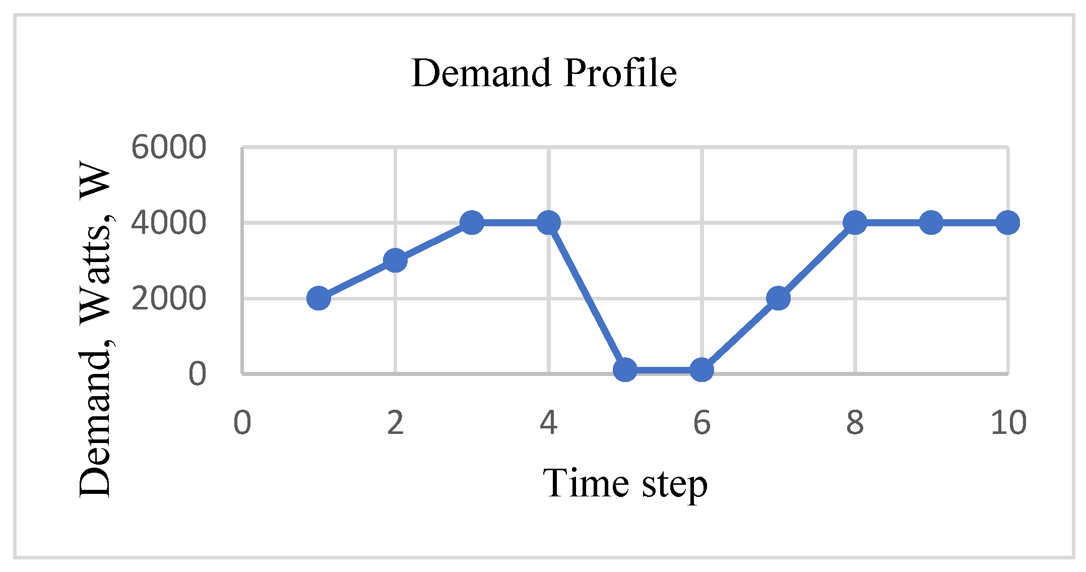
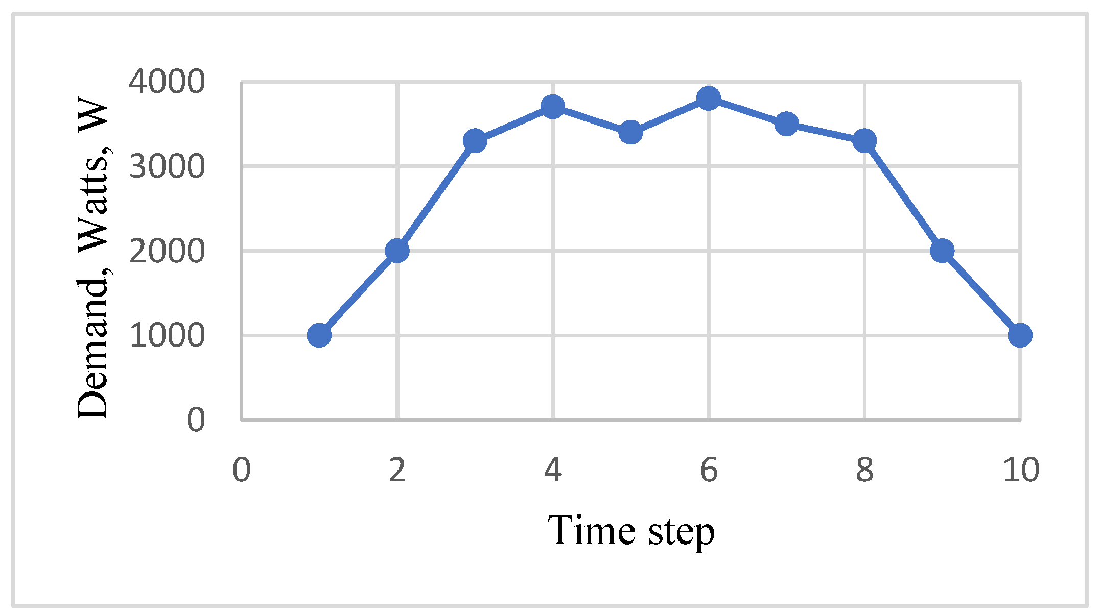
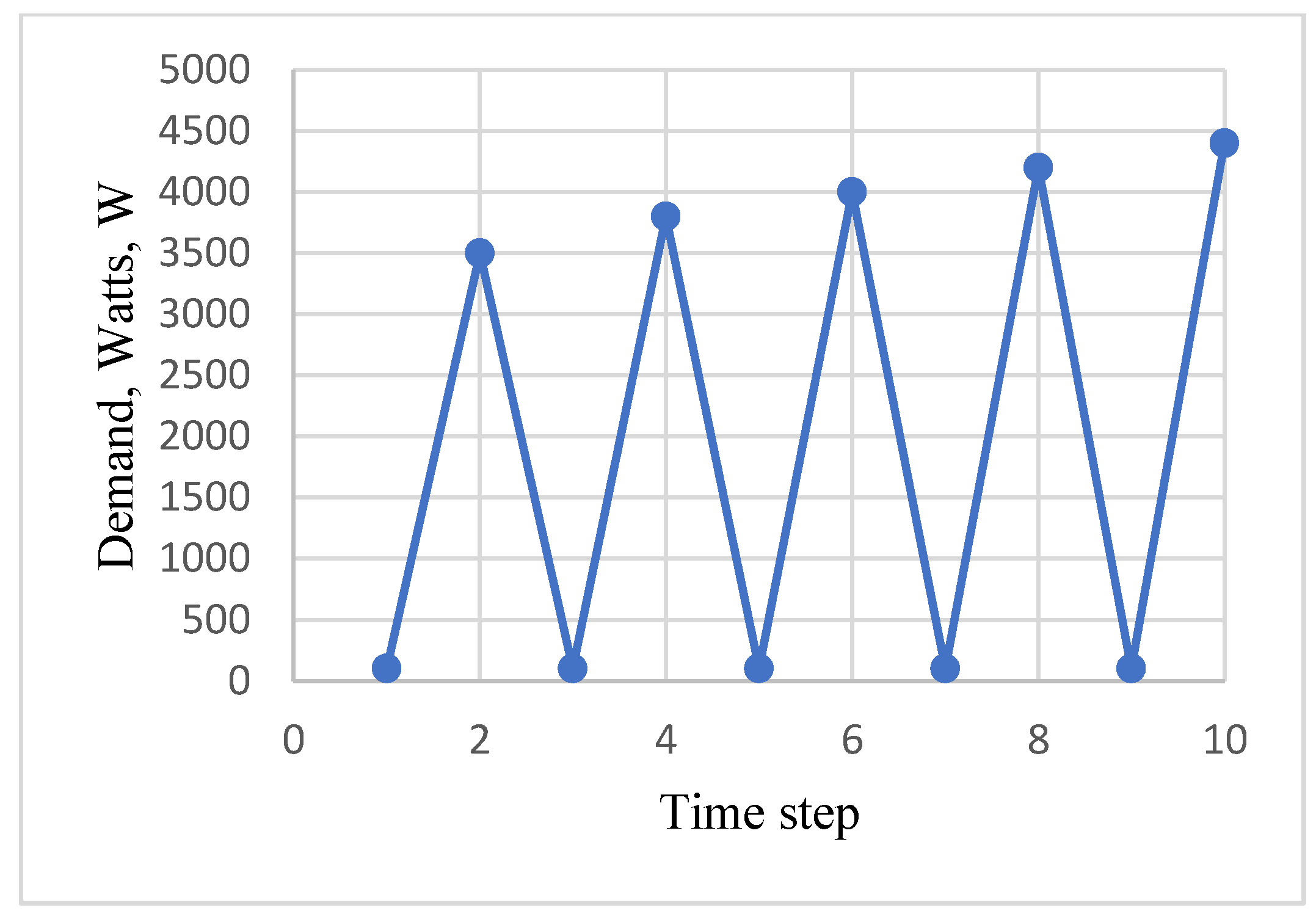
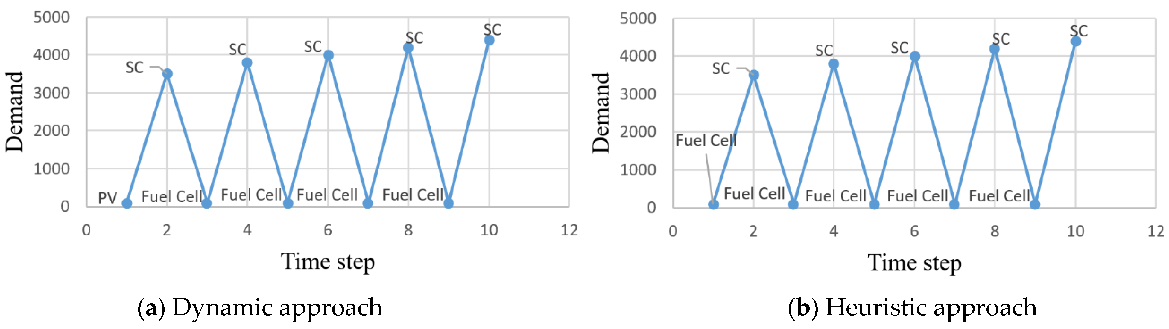
The following simulation represents the situation where a drone must travel to a specific location to pick up an object and return the object to the drone’s base. During this simulation, ideal conditions are considered where the drone does not face any disturbances or turbulence during its flight. The assumed demand profile for this simulation is shown in Figure 1. Initially, the drone starts traveling to the location where the object is located. At time step 4, the drone reaches the object’s location and descends to pick up the desired object. After the drone picks up the object, it continues its flight to return to its base.
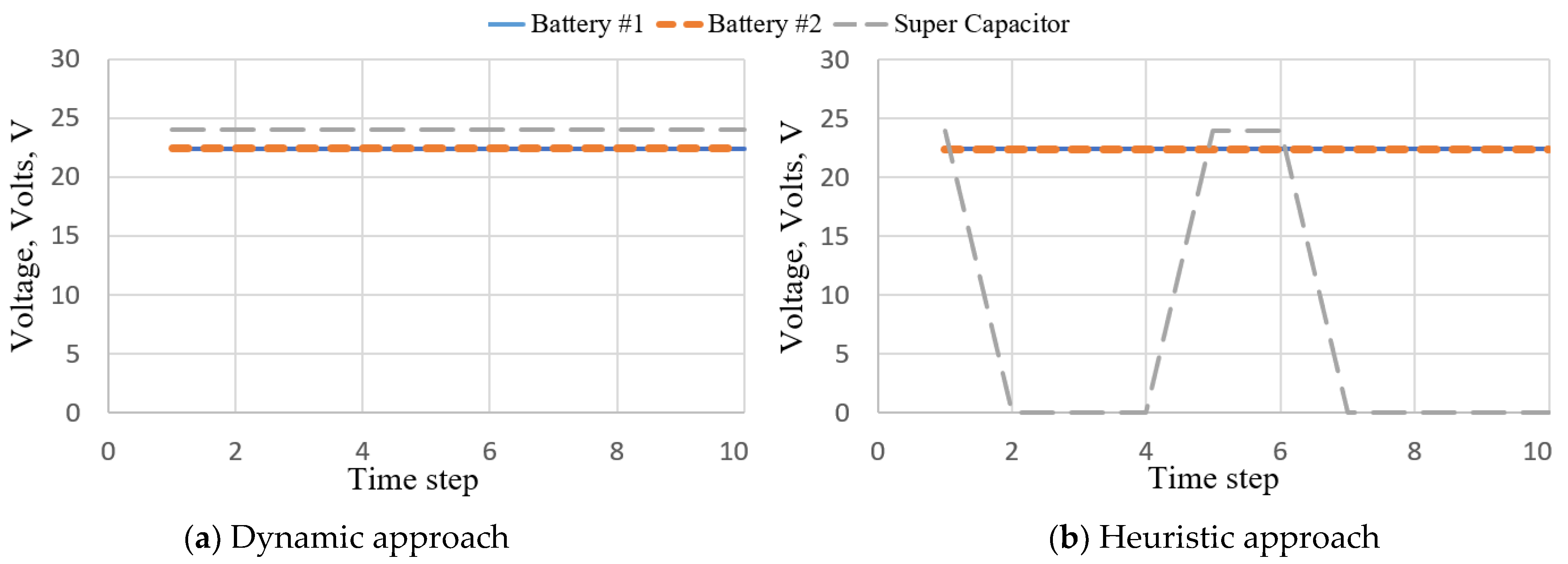
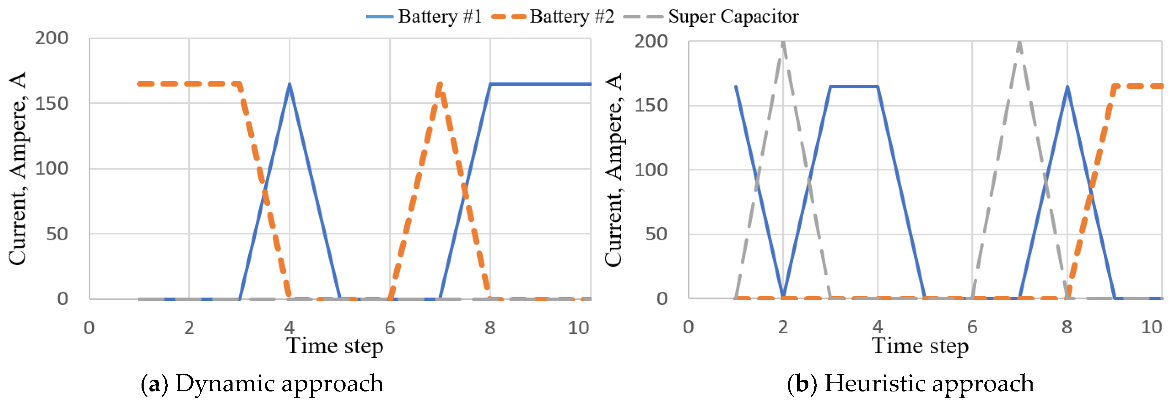
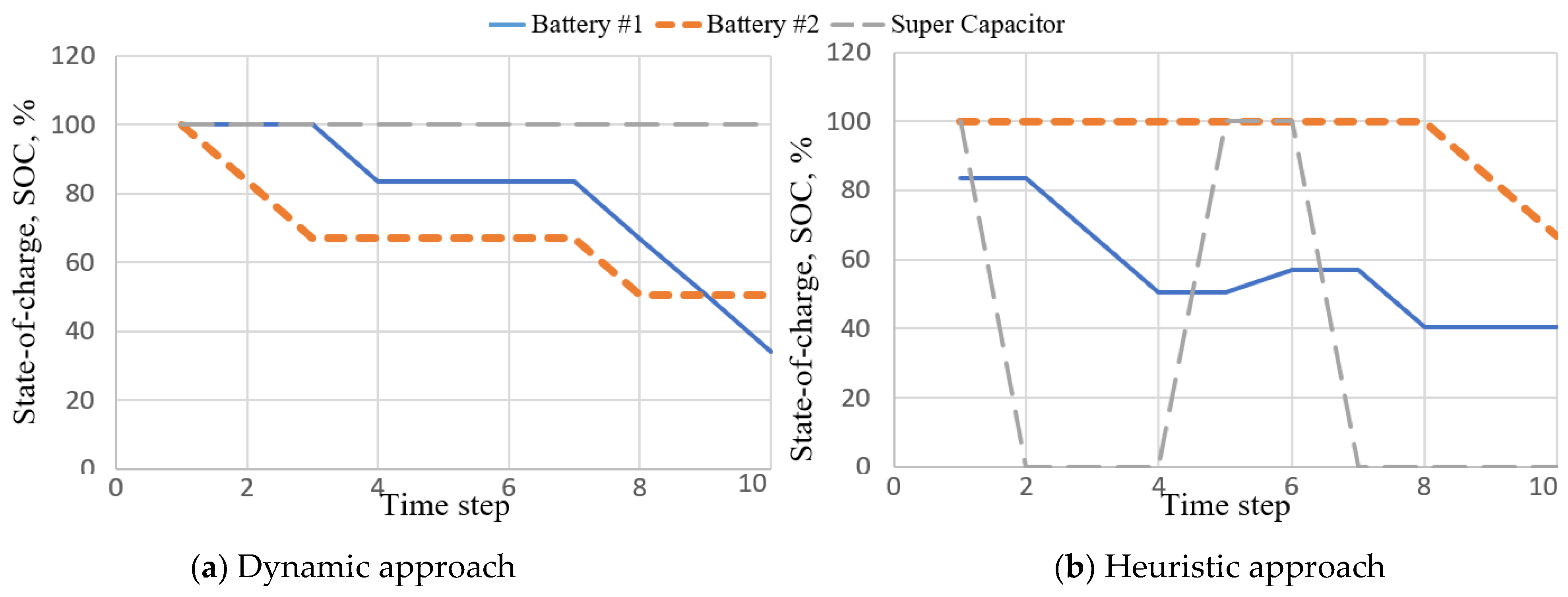
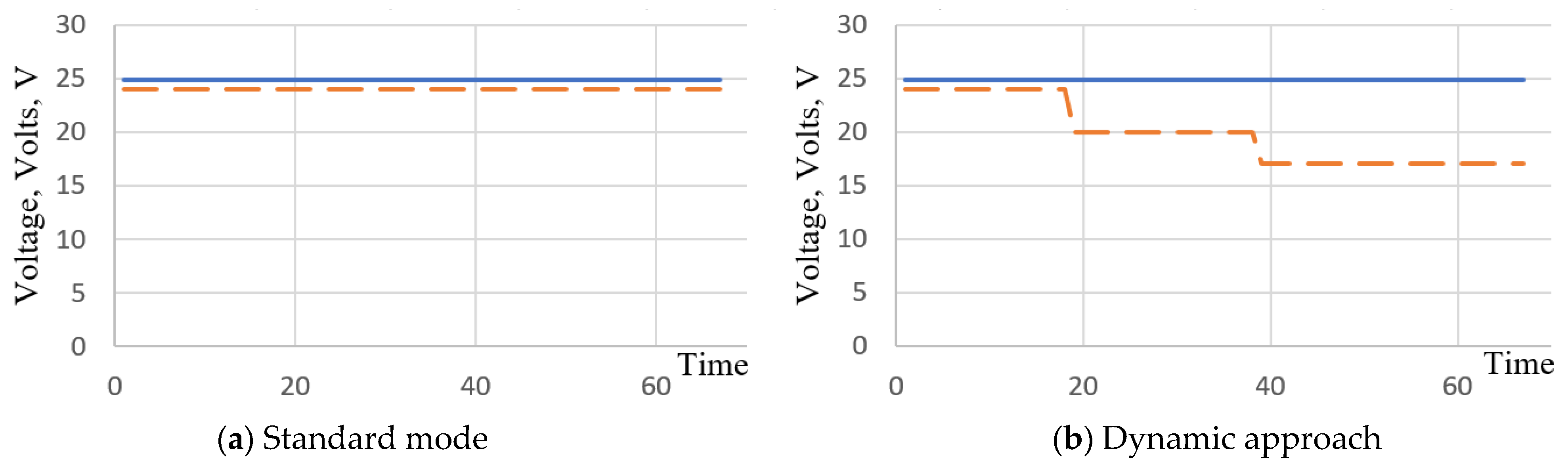
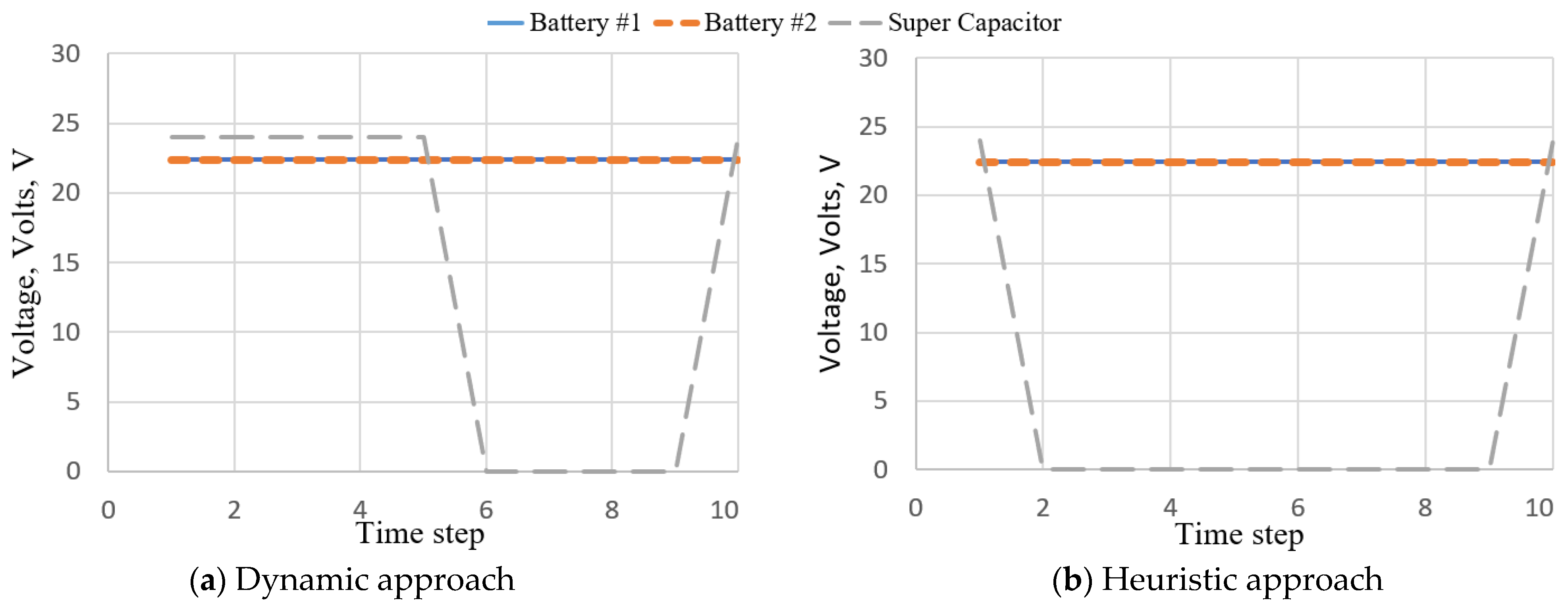
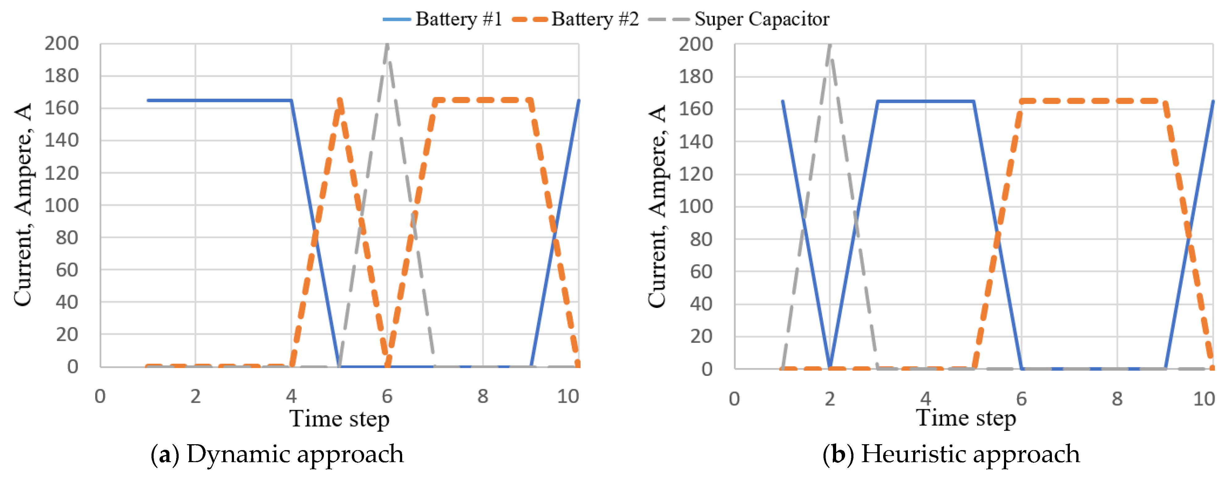
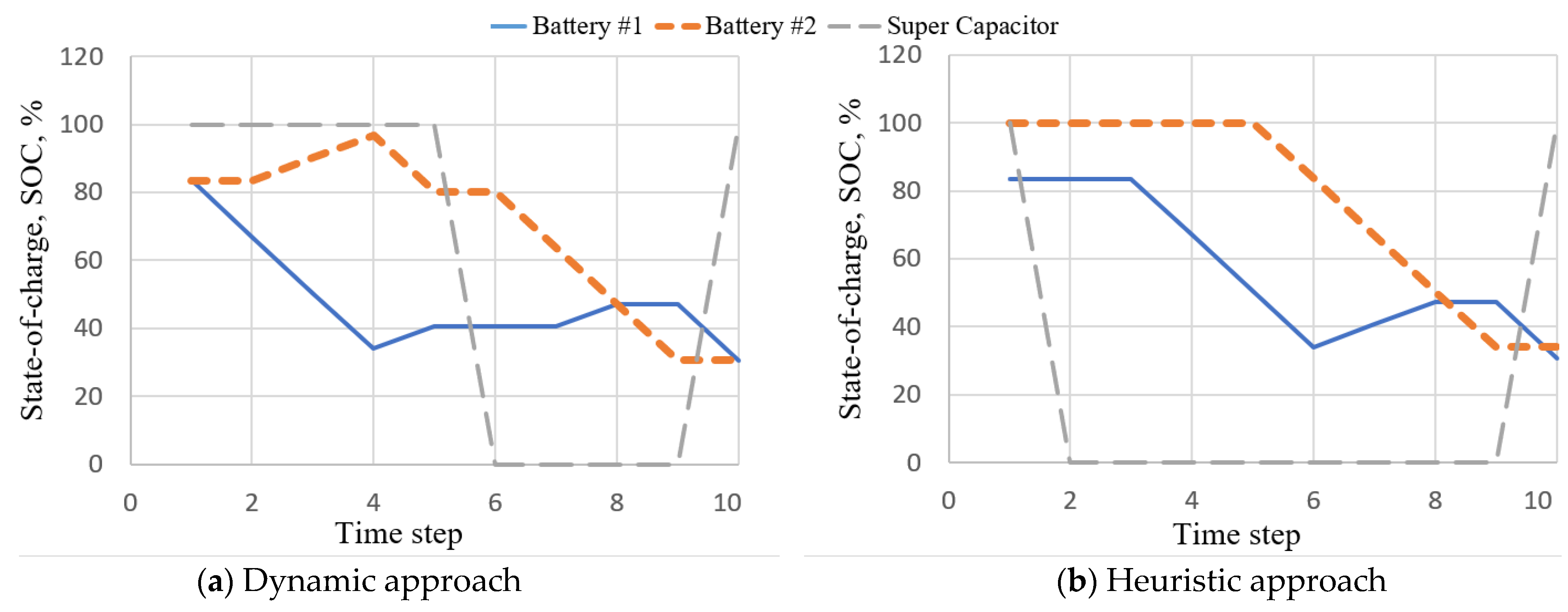
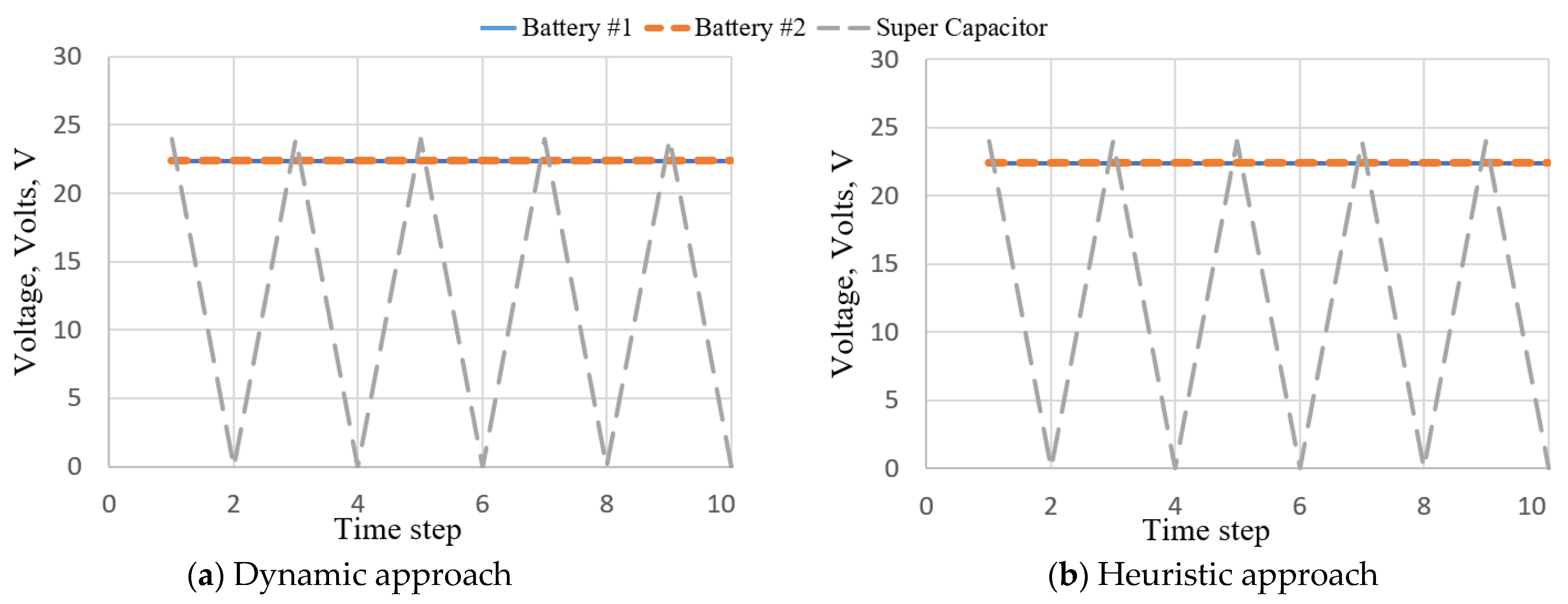
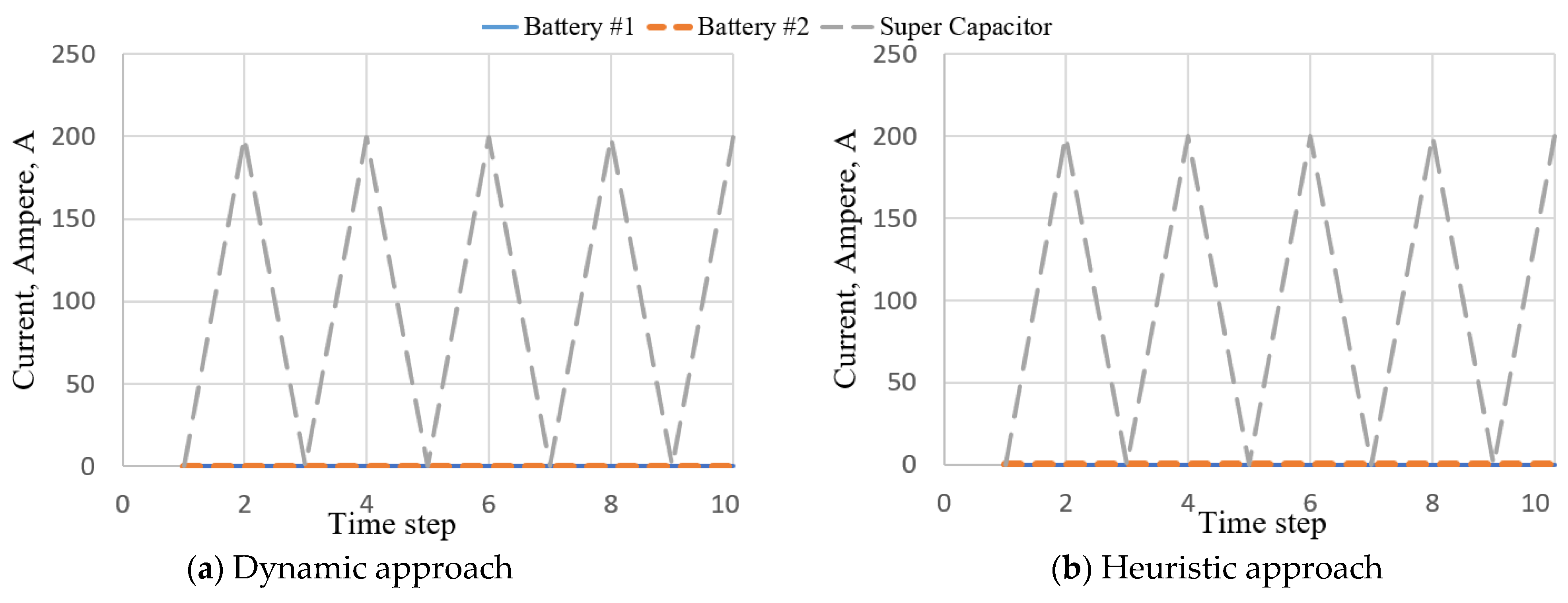
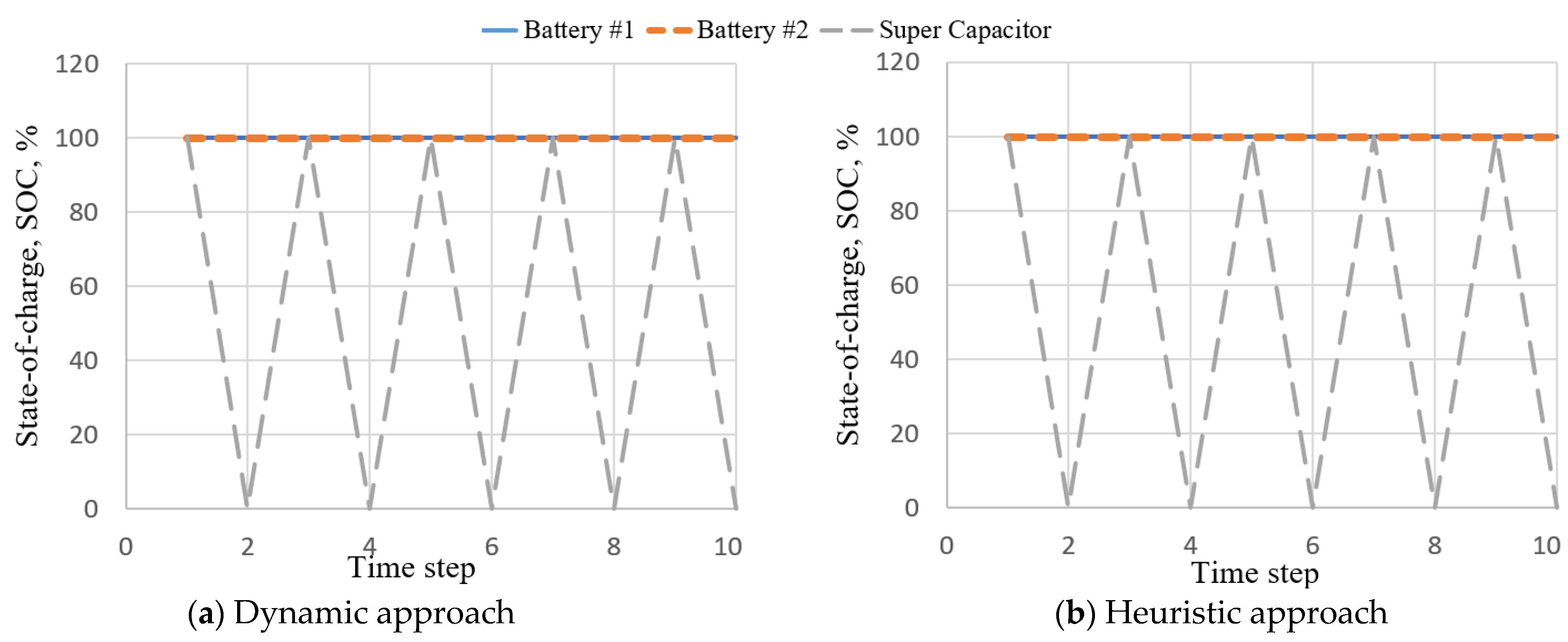
Figure 2, Figure 3 and Figure 4 display the system voltages, current, and state-of-charge, respectively, for both the dynamic and heuristic approaches. The switching sequence generated by the dynamic approach chose not to use the super capacitor. As for the current, as the super capacitor was not used by the dynamic approach, the current remains 0 while the currents of the batteries vary as they are being used. However, in the heuristic approach, both batteries and the super capacitor were used; therefore, their currents vary accordingly.
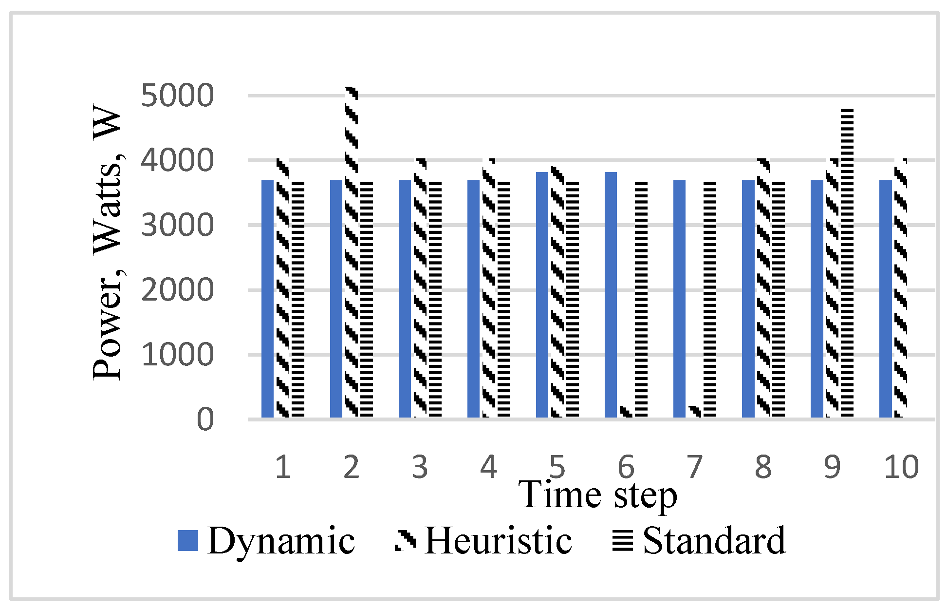
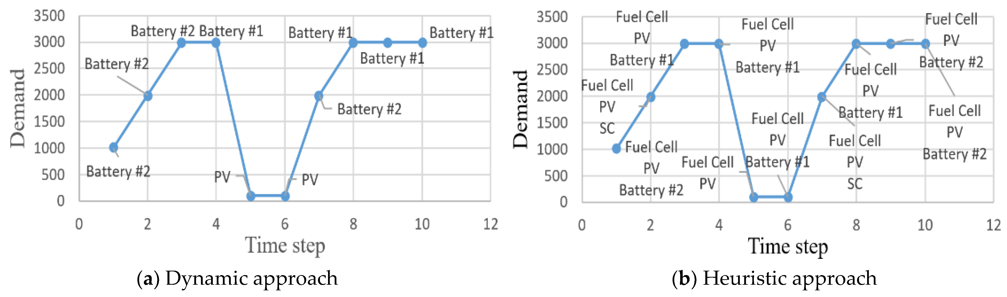
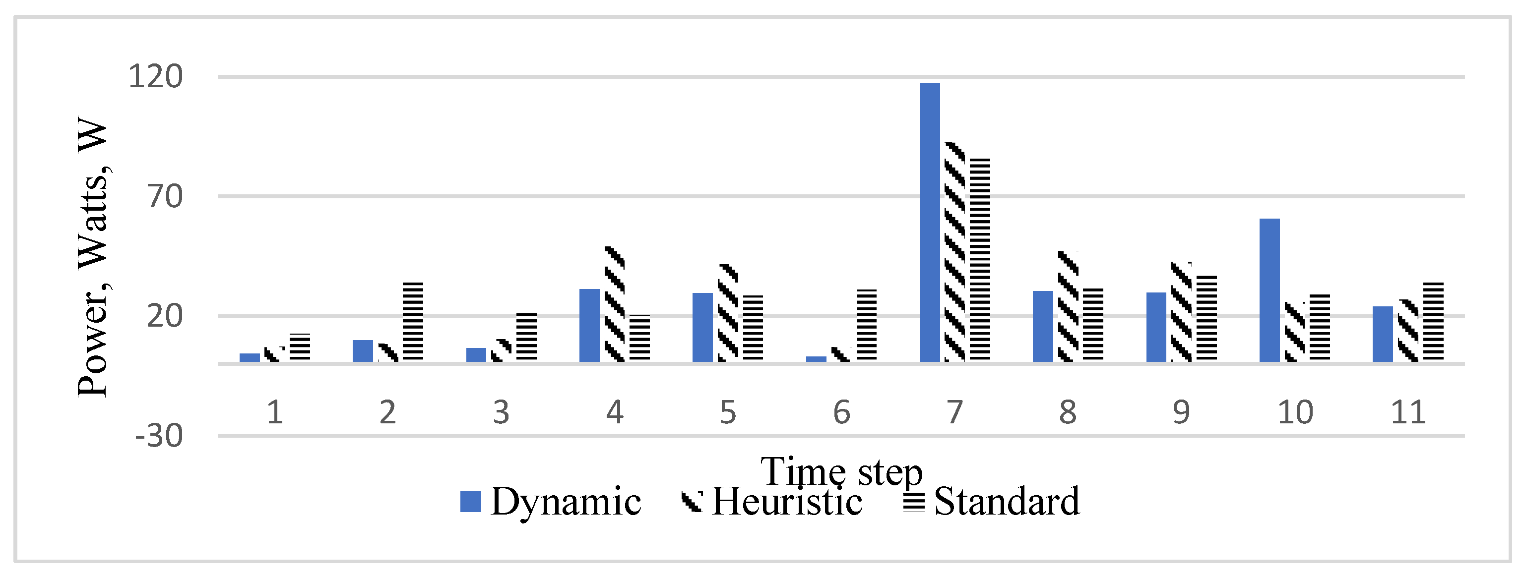
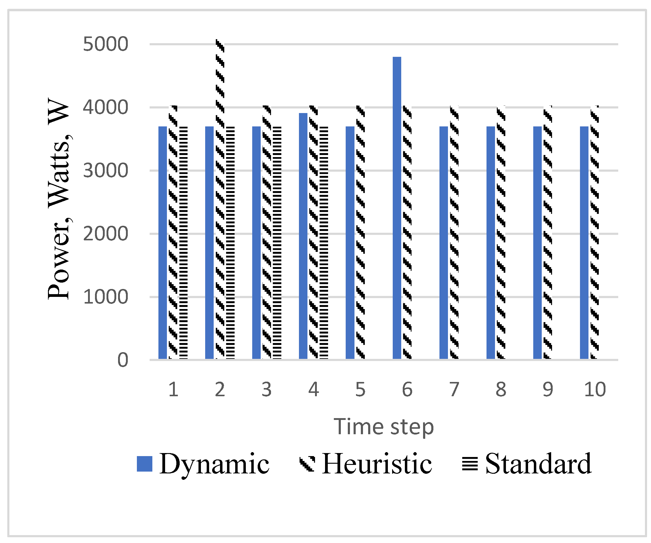
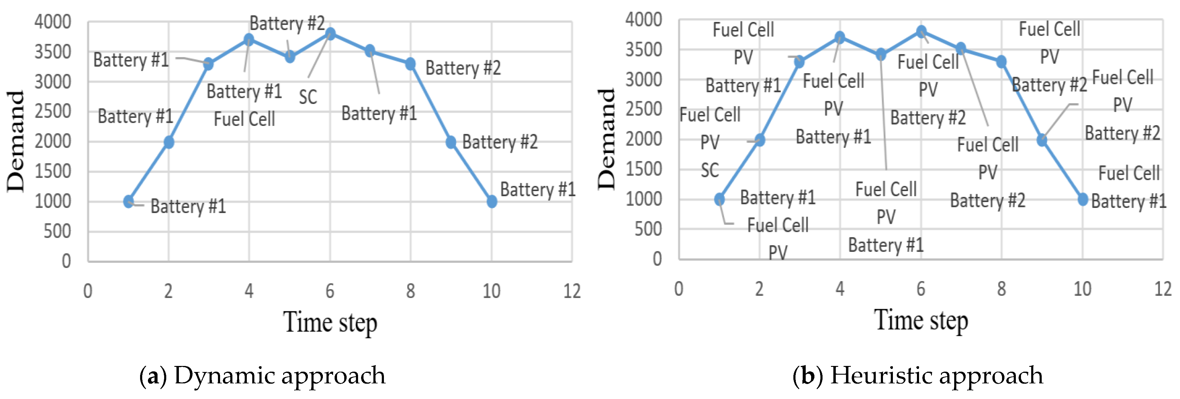
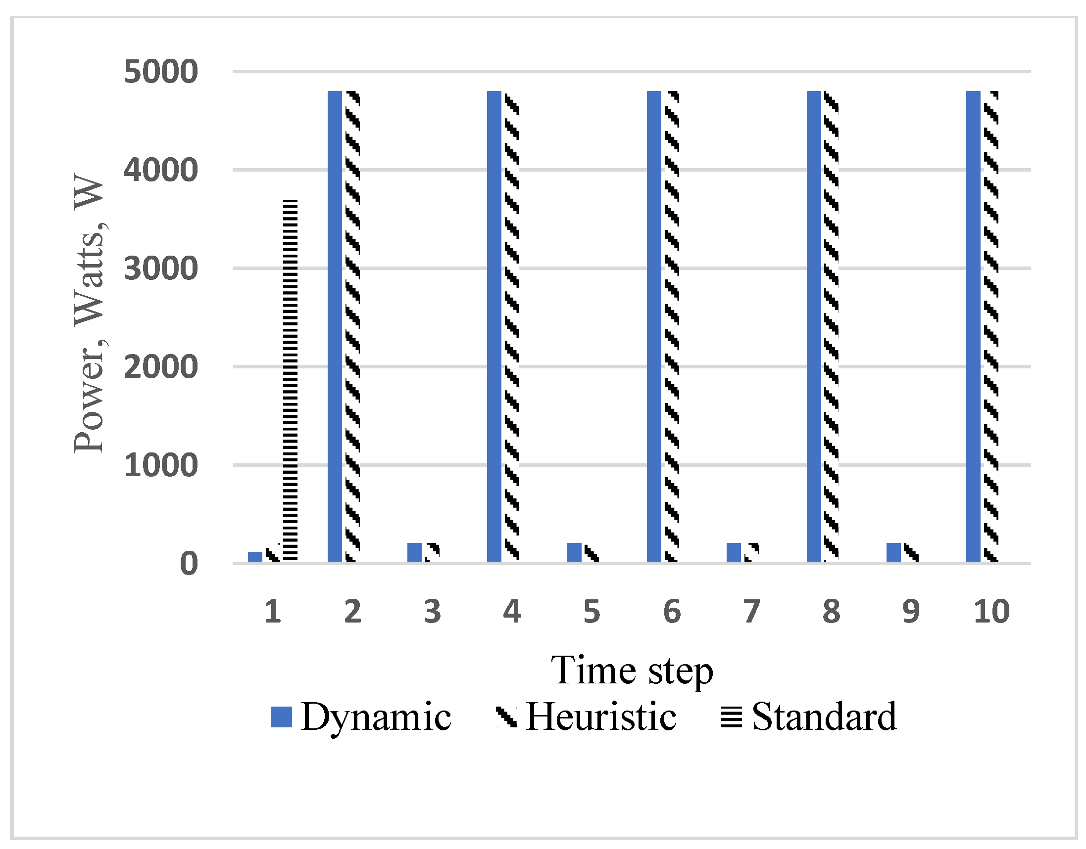
In the object pickup simulation, both the switching sequences of the dynamic approach and heuristic approach were able to meet the demand of the drone, but that of the standard approach did not. After both batteries and the super capacitor were completely depleted, the standard approach was unable to meet the demand of the drone in the 10th time instance. However, although both the switching sequences of the dynamic approach and heuristic approach met the demand, the dynamic approach provided a sequence of switching superior to that of the heuristic approach. The obtained objective function value of the dynamic approach was 9% lower with a value of 6536.2, while the heuristic approach was 7123.3. However, the switching sequences of the heuristic approach had a lower average power consumption of 3361.2 W compared to the dynamic approach’s 3720 W. This was due to the switching sequence of the dynamic approach resulting in significant power consumption in time steps 6 and 7. From Figure 4, the following can also be seen. The dynamic approach resulted in battery 1 having a SOC level of around 35% and battery 2 with a SOC level of around 50% after 10 s. While the SOC level of the supercapacitor was unchanged and remained at 100% throughout the time period. It is worth noting is that none of the batteries enter charging. In contrast, the heuristic approach seems to favor using the supercapacitor as a result of which the supercapacitor is completely discharged, re-charged, and discharged to SOC level zero again within the ten second time period. Battery 1 ends at a SOC level of 40%, and battery 2 ends at a SOC level of around 70%. The differences in behavior can be attributed to the optimization of the objective function value as mentioned above. The power used to meet the demand of the drone during each time step is shown in Figure 5. Figure 6 shows as additional examples the switching sequence and the sources used to meet demand shown in Figure 6a,b at each time step.
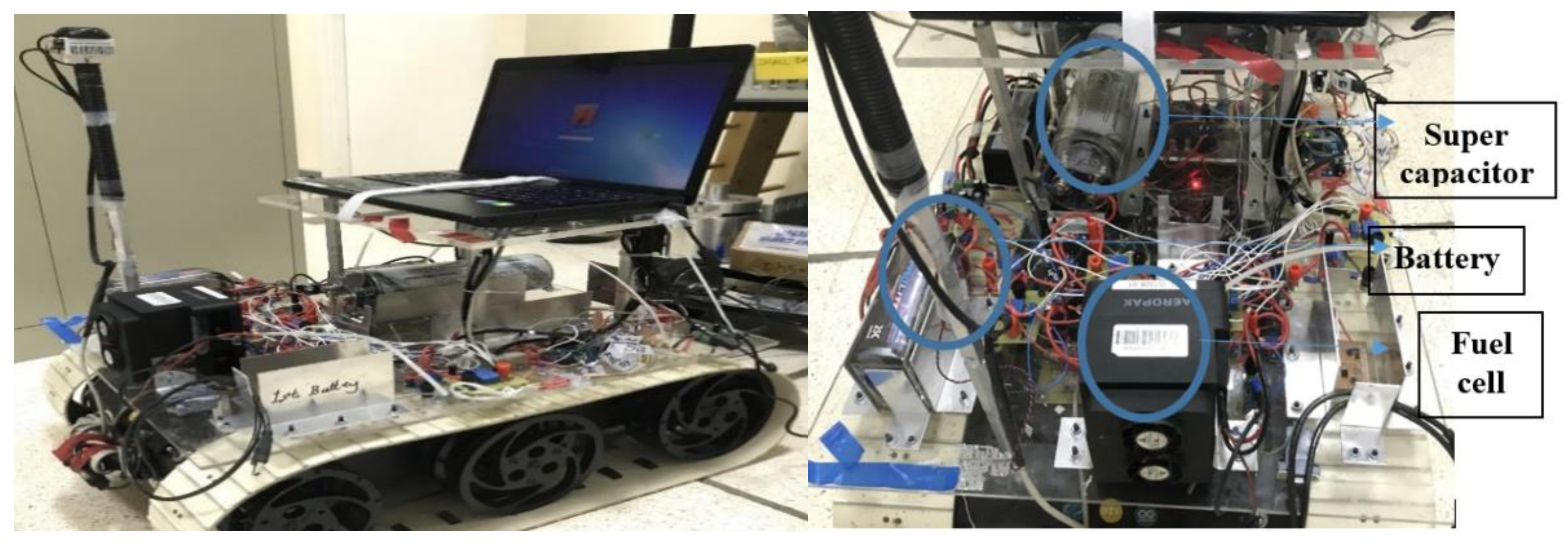
4.2. Experimental Work—On a Multi-Energy Source Ground Robot
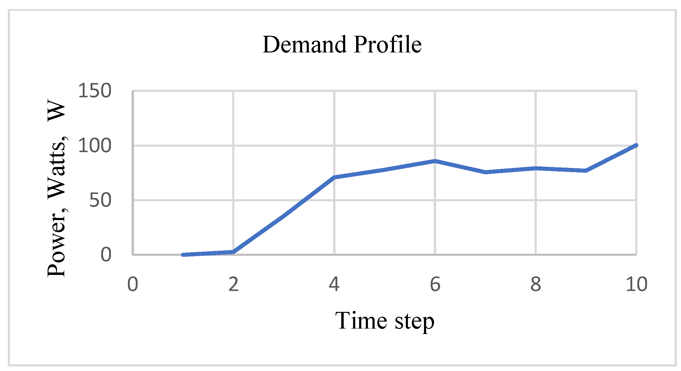
The following experiment was conducted on a ground robot shown in Figure 7. The ground robot contains three sources: batteries, super capacitor, and fuel cell. The robot was run in remote-control mode while conducting the tests. The robot was controlled by the remote controller to move around a lab bench in a rectangular path. The demand profile for all tests is shown in Figure 8.
For experimental work, a multi-energy source ground robot was preferred over a drone because of several factors: i.e., (i) limitations related to drone flight height and seeking clearances for flight paths at certain heights, (ii) even if an accurate flight power demand profile was obtained by flying a drone in good weather conditions, the actual flight power demand profile obtained when trying to verify results–cannot be guaranteed because the weather may change and sudden wind gusts may introduce power demand, not accounted for when solving for the dynamic programming solution, and (iii) it is also possible that the wind disturbances introduce differences in the demand profiles when performing an experiment with the heuristic approach, and entirely different power demand profile disturbances occur because of wind gusts when testing the dynamic approach. So, to make a comparison between the proposed approaches, which is free from random power surges due to weather effects, a ground robot with multiple energy sources was favored. Also, it is worth noting that when considering a drone, the demand profile can be easily calculated from first principles, as seen in Equation (15). But when considering a ground robot we have to actually run the robot around a path and acquire a demand curve. This is the procedure followed to get the curve in Figure 8, and therefore it is different from the curve in Figure 1. Please note that the developed approaches are not profile-specific, and can compute a switching sequence for a given demand profile. The demand profile was uploaded to both the dynamic and heuristic algorithm to obtain a switching sequence. The ground robot has a controller which supplies a given amount of current to the motors if it is given a reference current. The two motors on the robot chassis (one for controlling left side wheel speeds, and one for controlling right side wheel speeds) rotate clockwise or anticlockwise depending on the current received. Based on the direction of the rotation of the motors and the speed of rotation, the robot can be made to move in straight lines, curves, or in circles. This is extremely common in robotics literature and hence the details of the driving process (called differential drive) are not included here. However, there is not necessarily a controller that controls where the current comes from. The switching sequences generated by the dynamic and heuristic approaches tell this same lower level controller what sources to use to supply the required current; to satisfy the demand and still reduce the average power consumption across the sources. The switching sequences were then uploaded to the main controller of the ground robot, an Arduino microcontroller that controls the switches attached to the sources. After the switching sequence was uploaded, the ground robot performed a lap along the rectangular path. The power consumption across all sources after the ground robot completed a lap with the uploaded switching sequences was then compared with the standard mode of operation. For a ground robot, the standard mode of operation assumes no scheduling; however the needed power is first supplied by the battery until it’s completely depleted then moving to the other available sources.
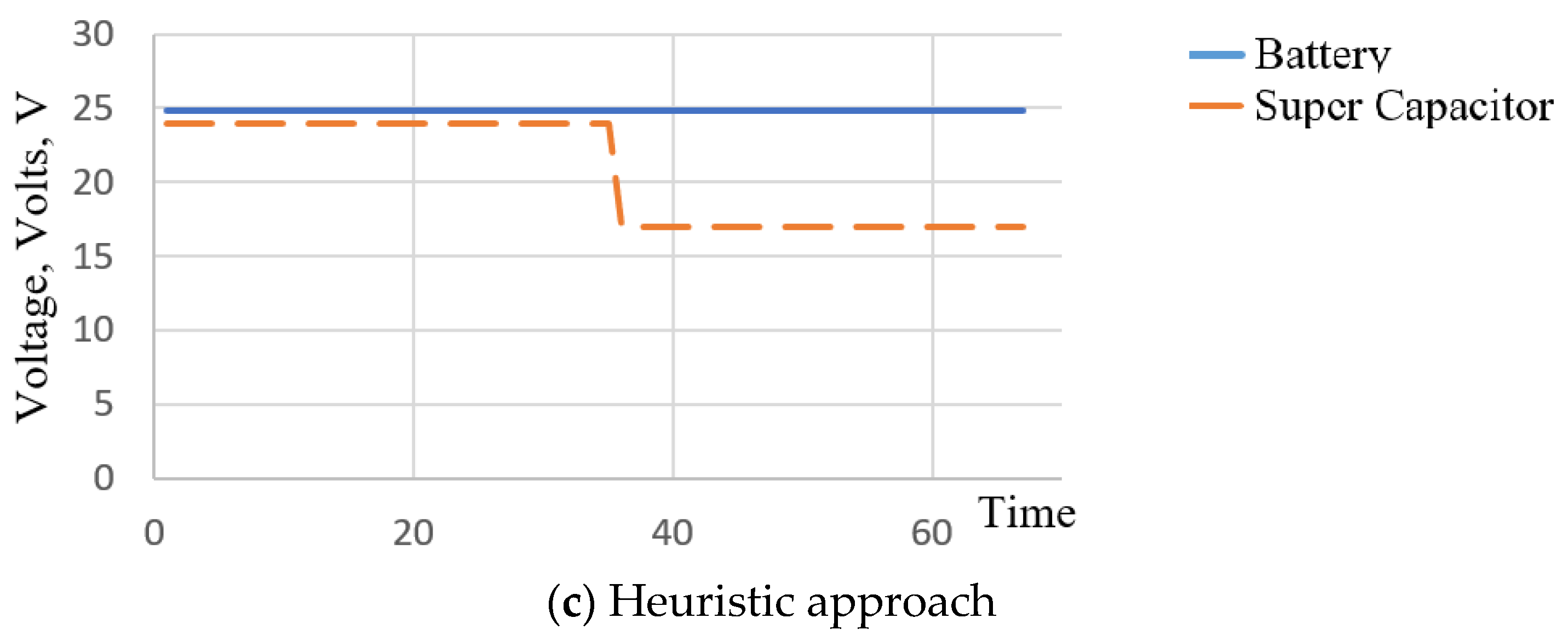
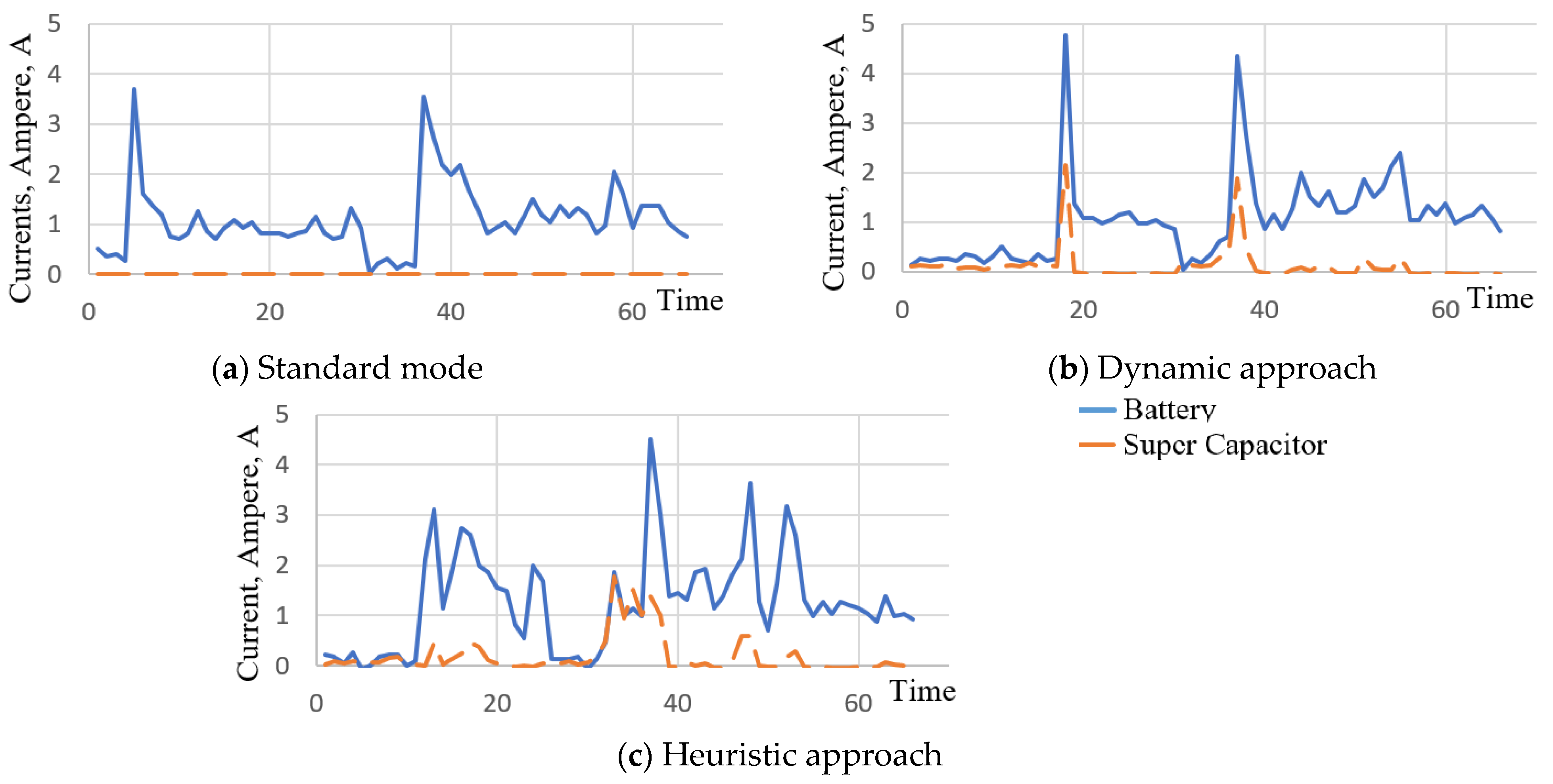
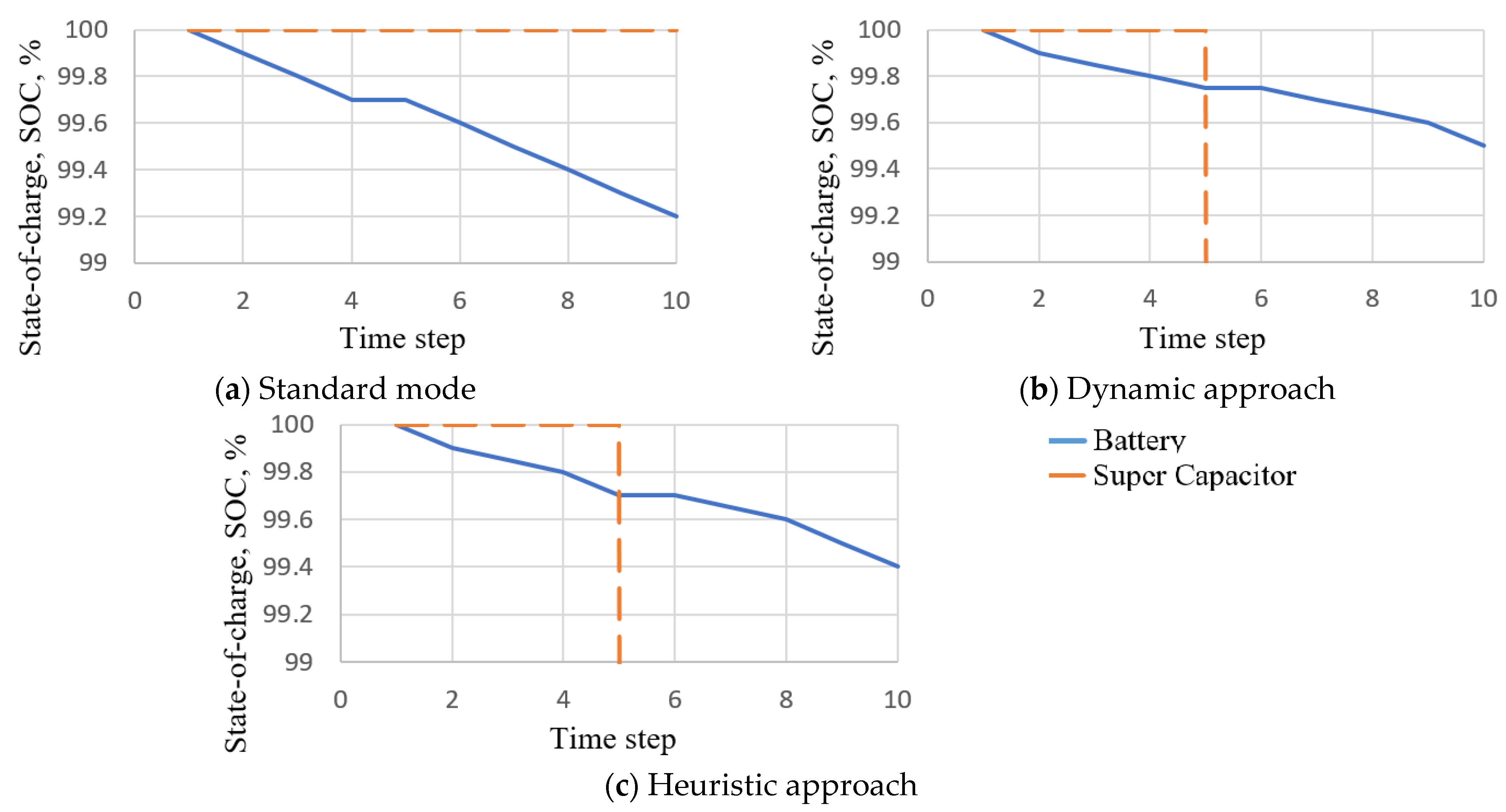
Figure 9, Figure 10 and Figure 11 display the system voltages, current, and state-of-charge, respectively, for the standard mode, the dynamic approach, and the heuristic approach. The standard mode of operation did not involve the super capacitor in meeting the demand of the ground robot. However, the dynamic programming approach and heuristic approach did. As for the current, the use of the super capacitor by the dynamic programming approach and heuristic approach is apparent in Figure 10. The state-of-charge of the battery decreases most in the standard mode of operation, reaching 99.2%.
The standard mode of operation of the ground robot relied solely on the battery to meet the demand. On the other hand, the switching sequence of the dynamic approach chose to use the battery and super capacitor to meet the demand, while the switching sequence of the heuristic approach chose all three sources. Although not visible in the current plots in Figure 10c, it can be seen from the algorithm of the heuristic approach proposed that the fuel cell is chosen by the heuristic approach at all times. Additionally, the current plots for the fuel cell are not shown because the fuel cell unit functions as a base load unit. This is because the fuel cell cannot be turned on/off very quick and has a hydrogen pressure regulator attached to its hydrogen input lines, which maintains a certain amount of gas flow, so the terminal voltage of the fuel cell remains constant, and the fuel cell supplies a certain amount of power. Thus in the heuristic approach, the fuel cell is used as a based load handling device, and the current for the fuel cell is not shown because depending on the overall circuit impedances, and depending on which other source is active, the fuel cell will supply the remainder of the load, and it is not subjected to rapid starts/stops in operation. The switching sequence of the standard mode of operation resulted in the highest average power consumption from the sources, 33.3 W. However, the dynamic approach generated a switching sequence that resulted in a 5.5% decrease in the average power consumption compared to the standard mode of operation due to the voltage dynamics of the sources. Similarly, the switching sequence of the heuristic approach was able to reduce the average power consumption by 2.5%, which is shown in Figure 12. Furthermore, the run time of the ground robot should increase since the system is less dependent on only one source to satisfy the demand.
5. Conclusions
This paper is concerned with multi source power systems consisting of batteries, super capacitors, a hydrogen fuel cell, and a photovoltaic cell. The usage of each of the sources is controlled by turning connected switches on or off as needed to supply the needed power demand of the system. A mathematical model was developed for the efficient energy management of the integrated sources, generating an optimal switching sequence between the sources. Two methods have been developed to solve for the optimal switching sequence.
The first method uses a dynamic mathematical model solved using Lingo to minimize the running cost of the system by generating a switching sequence. The second method uses a heuristic approach, where a set of rules were used to generate the switching sequence. The heuristic algorithm was primarily tested on Matlab. The switching sequences generated by the dynamic approach resulted in power consumption that was on average 9% lower than those of the heuristic approach. However, the main advantage introduced by the heuristic algorithm was the short computational time needed to generate the switching sequence between the sources. The developed approaches were implemented offline before running the system, but can be implemented online. To be implemented online, the algorithms would require readings of the system’s behavior and demand to generate the optimal switching sequence.
Additionally, both approaches were tested in simulations of a drone flight scenario, and also experimentally tested on a multi-energy source ground robot. The developed dynamic model was capable of generating a switching sequence that minimized the power dissipation of the energy sources for the illustrative simulation examples of a drone, while the standard mode of operation was failed to provide the needed power. Also, the model was able to prolong the simulated flight time of the drone by charging the batteries and the super capacitor as needed depending on the demand profile. The switching sequences generated by the heuristic algorithm were also able to prolong the flight time in the simulation tests related to the drone, and minimize the power dissipation of the energy sources; but not as well as those of the dynamic modeling approach.
Both the dynamic modeling, and heuristic approaches, when tested on a multi-energy source ground robot, were able to generate switching sequences that minimize the power dissipation by reducing the average power consumption across the sources due to the voltage dynamics of the different sources. However, the dynamic approach’s switching sequence resulted in the most significant reduction in the average power consumption; 5.5% lower average power consumption compared to the standard mode of operation of the robot. The switching sequence of the heuristic approach was also able to reduce the average power consumption by 2.5% compared to the standard mode of operation.
The limitations faced in this work include the length of the simulations conducted. Due to the large computing power required by the dynamic model based approach, the simulations were conducted for only fifty seconds. However, with access to more computing power, better switching sequences could be generated that provide a further reduction in the running cost of the system. Additionally, future work could include the real-time management of the sources integrated into the system, alongside continuous readings of the behavior of the system while it is being used. By implementing the real-time management of the sources, the system could become more responsive to fluctuations in demand.
Author Contributions
O.S.: Conceptualization, methodology, programming and writing the original draft. A.S. and S.M.: Conceptualization, methodology, and finalizing the manuscript. All authors have read and agreed to the published version of the manuscript.
Funding
The authors received no specific funding for this work.
Institutional Review Board Statement
Not applicable.
Informed Consent Statement
Not applicable. This article does not contain any studies with human participants or animals performed by any of the authors.
Data Availability Statement
The data presented in this study are available on request from the corresponding author.
Conflicts of Interest
The authors have no conflict of interest to declare.
Abbreviations
| k | Time step |
| ∆t | Step size (seconds), using this and k we get time t = k∆t seconds |
| N | Number of time steps |
| j | Battery index ∀ j{1,2} |
| τ | Time constant of the super capacitor |
| w | Power source relative weight |
| Bj | Battery number j |
| C | Super capacitor |
| PV | Photovoltaic cell |
| FC | Fuel cell |
| A binary variable that equals 1, if battery j is supplying the demand of the system at time step k, 0 otherwise | |
| A binary variable that equals 1, if battery j is being charged from the system time step k, 0 otherwise | |
| A binary variable that equals 1, if the super capacitor is supplying the demand of the system at time step k, 0 otherwise | |
| A binary variable that equals 1, if the super capacitor is being charged from the system at time step k, 0 otherwise | |
| A binary variable that equals 1, if the photovoltaic cell is supplying the demand of the system at time step k, 0 otherwise | |
| A binary variable that equals 1, if the fuel cell is supplying the demand of the system at time step k, 0 otherwise | |
| State of charge of the battery j at time step k | |
| State of charge of the super capacitor at time step k | |
| Voltage of the battery j at time step k | |
| Current of the battery j at time step k | |
| Power supplied by the battery j at time step k | |
| Voltage of the super capacitor at time step k | |
| Current of the super capacitor at time step k | |
| Power supplied by the super capacitor at time step k | |
| Power supplied by the photovoltaic cell at time step k | |
| Voltage of the fuel cell at time step k | |
| Current of the fuel cell at time step k | |
| Power supplied by the fuel cell at time step k | |
| Power demanded by the system at time step k |
Appendix A. Illustrative Example: Altitude Maintenance
The following simulation represents the situation where a drone must maintain a certain height above the ground for a short period of time. During its flight, the drone faces turbulence causing fluctuations in the demand profile. The demand profile of this simulation is shown in Figure A1; the drone starts ascending to the required height, thus causing an increase in the energy of the drone. At time step 3, the drone reaches the required height and tries to maintain it for five time steps. However, the drone faces significant turbulence causing fluctuations in the height it maintains, which is represented in the demand profile. Finally, the drone begins to descend back to its base.
Figure A1.
Demand profile.

Figure A2, Figure A3 and Figure A4 display the system voltages, current, and state-of-charge, respectively, for both the dynamic and heuristic approaches.
Figure A2.
System voltage for simulation 2.

Figure A3.
System currents.

Figure A4.
System state-of-charges.

In the altitude maintenance simulation, both the switching sequences of both the dynamic and heuristic approaches were able to meet the demand of the drone, but that of the standard approach did not. While the drone was attempting to maintain the required altitude, the demand was higher than the power that the sources could provide separately. Therefore, resulting in the standard approach’s inability to meet the demand of the drone. Additionally, in this simulation, the dynamic approach performed better than the heuristic approach. The dynamic approach provided a sequence of switching between the sources that resulted in an objective function value of 8301.2, while the heuristic approach was 8501.3. Additionally, the average power consumption obtained using the dynamic approach was 3827.4 W, while the heuristic approached resulted in 4136.4 W. The power used to meet the demand of the drone during each time step is shown in Figure A5. The switching sequence and sources used to meet demand are shown in Figure A6
Figure A5.
Power consumption comparison for simulation 2.

Figure A6.
Switching sequence and sources used to meet demand.

Appendix B. Illustrative Example-Multiple Object Pickup
The following simulation represents a drone conducting multiple pickups of objects located in close proximity to each other. The demand profile of this simulation is shown in Figure A7. The weights assigned to the sources in the objective function have to be updated to account for the multiple spikes of demand during the drone’s flight. As shown in the demand profile, the drone starts traveling to the location of the first object is located. At time step 2, the drone reaches the object’s location and descends to pick up the object. After the drone picks up the object, it proceeds to proceed to pick up the next object until all four objects are obtained. The demand increases as the drone picks up each object, as the load carried by the drone increases.
Figure A7.
Demand Profile for simulation 3.

Figure A8, Figure A9 and Figure A10 display the system voltage, current, and state-of-charge, respectively, for both the dynamic and heuristic approaches. In this simulation, the switching sequence generated by the dynamic approach chose to mainly use the super capacitor to meet the demand of the drone, as did the heuristic approach. It can be noted that the super capacitor’s current varies in a similar manner to that of the drone’s demand as the super capacitor was mainly used by both the dynamic and heuristic approaches. As for the state-of-charge, since the batteries were not used in this example, the state-of-charge of the batteries remains 100% while the super capacitor is charged and discharged multiple times to meet the demand.
Figure A8.
System voltage.

Figure A9.
System currents.

Figure A10.
System state-of-charges.

In the multiple object pickup simulation, both the switching sequences of the dynamic and heuristic approach were able to meet the demand of the drone, but that of the standard approach did not. The switching sequences of the standard approach were unable to meet the demand of the drone due to the multiple spikes in demand. During spikes in demand, the use of the super capacitor is preferred due to its rapid discharge rate making it best-equipped to handle spikes. The switching sequences of the dynamic and heuristic approaches both utilized the super capacitor to meet the spikes in demand of the drone.
Additionally, in both approaches, the super capacitor was charged when the demand was low so that it could be used during the next spike in demand. However, although both the methods performed similarly, the dynamic approach chose to use the photovoltaic cell in the first time step rather than the fuel cell to meet the demand. Therefore, resulting in an objective function value of 3499.2 and average power consumption of 2496 W for the switching sequence of the dynamic approach. On the other hand, the switching sequence of the heuristic approach resulted in an objective function value of 3517.5 and average power consumption of 2505 W. Therefore, resulting in slightly lower power consumption, which is shown in Figure A11. The switching sequence and sources used to meet demand are shown in Figure A12.
Figure A11.
Power consumption comparison.

Figure A12.
Switching sequence and sources used to meet demand.

References
- Malikopoulos, A.A. Supervisory Power Management Control Algorithms for Hybrid Electric Vehicles: A Survey. IEEE Trans. Intell. Transp. Syst. 2014, 15, 1869–1885. [Google Scholar] [CrossRef]
- Hu, X.; Murgovski, N.; Johannesson, L.M.; Egardt, B. Optimal Dimensioning and Power Management of a Fuel Cell/Battery Hybrid Bus via Convex Programming. IEEE/ASME Trans. Mechatronics 2015, 20, 457–468. [Google Scholar] [CrossRef]
- Naamane, A.; M’Sirdi, N.K. Improving Multiple Source Power Management Using State Flow Approach. Blockchain Technol. Innov. Bus. Process. 2013, 22, 779–785. [Google Scholar] [CrossRef]
- Keller, S.; Christmann, K.; Gonzalez, M.S.-A.; Heuer, A. A Modular Fuel Cell Battery Hybrid Propulsion System for Powering Small Utility Vehicles. In Proceedings of the 2017 IEEE Vehicle Power and Propulsion Conference (VPPC), Belfort, France, 14–17 December 2017; pp. 1–4. [Google Scholar]
- Chen, X.; Shi, M.; Zhou, J.; Chen, Y.; Zuo, W.; Wen, J.; He, H. Distributed Cooperative Control of Multiple Hybrid Energy Storage Systems in a DC Microgrid Using Consensus Protocol. IEEE Trans. Ind. Electron. 2019, 67, 1968–1979. [Google Scholar] [CrossRef]
- Suárez- Suarez-Velazquez, G.; Mejia-Ruiz, G.E.; Garcia-Vite, P.M. Control and Grid Connection of Fuel Cell Power System. In Proceedings of the 2020 IEEE International Autumn Meeting on Power, Electronics and Computing (ROPEC), Ixtapa, México, 4–6 November 2020; pp. 1–5. [Google Scholar]
- Ferrandez, S.M.; Harbison, T.; Weber, T.; Sturges, R.; Rich, R. Optimization of a truck-drone in tandem delivery network using k-means and genetic algorithm. J. Ind. Eng. Manag. 2016, 9, 374–388. [Google Scholar] [CrossRef] [Green Version]
- Masjosthusmann, C.; Kohler, U.; Decius, N.; Buker, U. A vehicle energy management system for a Battery Electric Vehicle. In Proceedings of the 2012 IEEE Vehicle Power and Propulsion Conference (VPPC), Seoul, Korea, 9–12 October 2012; pp. 339–344. [Google Scholar]
- Boutilier, J.J.; Brooks, S.C.; Janmohamed, A.; Byers, A.; Buick, J.; Zhan, C.; Schoellig, A.; Cheskes, S.; Morrison, L.J.; Chan, T.C.Y. Optimizing a Drone Network to Deliver Automated External Defibrillators. Circulation 2017, 135, 2454–2465. [Google Scholar] [CrossRef] [PubMed]
- Lee, J. Optimization of a modular drone delivery system. In Proceedings of the 2017 Annual IEEE International Systems Conference (SysCon), Montreal, QC, Canada, 24–27 April 2017; pp. 1–8. [Google Scholar]
- Banerjee, A.; Roychoudhury, A. Future of Mobile Software for Smartphones and Drones: Energy and Performance. In Proceedings of the 2017 IEEE/ACM 4th International Conference on Mobile Software Engineering and Systems (MOBILESoft), Buenos Aires, Argentina, 22–23 May 2017; pp. 1–12. [Google Scholar]
- Torreglosa, J.; Garcia, P.; Fernandez, L.; Jurado, F. Predictive Control for the Energy Management of a Fuel-Cell–Battery–Supercapacitor Tramway. IEEE Trans. Ind. Inform. 2014, 10, 276–285. [Google Scholar] [CrossRef]
- Xie, S.; Peng, J.; He, H. Plug-In Hybrid Electric Bus Energy Management Based on Stochastic Model Predictive Control. Energy Procedia 2017, 105, 2672–2677. [Google Scholar] [CrossRef]
- Hadj-Said, S.; Colin, G.; Ketfi-Cherif, A.; Chamaillard, Y. Convex Optimization for Energy Management of Parallel Hybrid Electric Vehicles. IFAC-PapersOnLine 2016, 49, 271–276. [Google Scholar] [CrossRef]
- Trovao, J.; Santos, V.; Antunes, C.; Pereirinha, P.; Jorge, H. A Real-Time Energy Management Architecture for Multisource Electric Vehicles. IEEE Trans. Ind. Electron. 2015, 62, 3223–3233. [Google Scholar] [CrossRef]
- Trovao, J.P.F.; Roux, M.-A.; Menard, E.; Dubois, M.R. Energy- and Power-Split Management of Dual Energy Storage System for a Three-Wheel Electric Vehicle. IEEE Trans. Veh. Technol. 2017, 66, 5540–5550. [Google Scholar] [CrossRef]
- Zhou, D.; Gao, F.; Ravey, A.; Al-Durra, A.; Simoes, M.G. Online energy management strategy of fuel cell hybrid electric vehicles based on time series prediction. In Proceedings of the 2017 IEEE Transportation Electrification Conference and Expo (ITEC), Chicago, IL, USA, 22–24 June 2017; pp. 113–118. [Google Scholar]
- Chen, Z.; Liu, W.; Yang, Y.; Chen, W. Online Energy Management of Plug-In Hybrid Electric Vehicles for Prolongation of All-Electric Range Based on Dynamic Programming. Math. Probl. Eng. 2015, 2015, 1–11. [Google Scholar] [CrossRef] [Green Version]
- Qin, F.; Li, W.; Hu, Y.; Xu, G. An Online Energy Management Control for Hybrid Electric Vehicles Based on Neuro-Dynamic Programming. Algorithms 2018, 11, 33. [Google Scholar] [CrossRef] [Green Version]
- Mathur, P.; Swartz, C.L.; Zyngier, D.; Welt, F. Robust online scheduling for optimal short-term operation of cascaded hydropower systems under uncertainty. J. Process. Control. 2021, 98, 52–65. [Google Scholar] [CrossRef]
- Park, S.; Zhang, L.; Chakraborty, S. Battery assignment and scheduling for drone delivery businesses. In Proceedings of the 2017 IEEE/ACM International Symposium on Low Power Electronics and Design (ISLPED), Taipei, Taiwan, 24–26 July 2017; pp. 1–6. [Google Scholar]
- Umetani, S.; Fukushima, Y.; Morita, H. A linear programming based heuristic algorithm for charge and discharge scheduling of electric vehicles in a building energy management system. Omega 2017, 67, 115–122. [Google Scholar] [CrossRef]
- Zhen, J.; Huang, G.; Li, W.; Wu, C.; Liu, Z. An optimization model design for energy systems planning andmanagement under considering air pollution control in TangshanCity, China. J. Process. Control 2016, 47, 58–77. [Google Scholar] [CrossRef]
- Vaccari, M.; Mancuso, G.; Riccardi, J.; Cantù, M.; Pannocchia, G. A Sequential Linear Programming algorithm for economicoptimization of Hybrid Renewable Energy Systems. J. Process. Control 2019, 74, 189–201. [Google Scholar] [CrossRef]
- Chen, M.; Rincon-Mora, G. Accurate Electrical Battery Model Capable of Predicting Runtime and I–V Performance. IEEE Trans. Energy Convers. 2006, 21, 504–511. [Google Scholar] [CrossRef]
- Schaltz, E.; Khaligh, A.; Rasmussen, P.O. Influence of Battery/Ultracapacitor Energy-Storage Sizing on Battery Lifetime in a Fuel Cell Hybrid Electric Vehicle. IEEE Trans. Veh. Technol. 2009, 58, 3882–3891. [Google Scholar] [CrossRef]
- Lami, M.; Shamayleh, A.; Mukhopadhyay, S. Minimizing the state of health degradation of Li-ion batteries onboard low earth orbit satellites. Soft Comput. 2019, 24, 4131–4147. [Google Scholar] [CrossRef]
- Bernard, J.; Delprat, S.; Buchi, F.; Guerra, T.M. Fuel-Cell Hybrid Powertrain: Toward Minimization of Hydrogen Consumption. IEEE Trans. Veh. Technol. 2009, 58, 3168–3176. [Google Scholar] [CrossRef]
- Pukrushpan, J. Modeling and Control of Fuel Cell Systems and Fuel Processors; University of Michigan: Ann Arbor, MI, USA, 2003. [Google Scholar]
- Spyker, R.; Nelms, R. Classical equivalent circuit parameters for a double-layer capacitor. IEEE Trans. Aerosp. Electron. Syst. 2000, 36, 829–836. [Google Scholar] [CrossRef]
- Amjadi, Z.; Williamson, S.S. Power-Electronics-Based Solutions for Plug-in Hybrid Electric Vehicle Energy Storage and Management Systems. IEEE Trans. Ind. Electron. 2010, 57, 608–616. [Google Scholar] [CrossRef]
- Saaty, T. The Analytic Hierarchy Process; McGraw-Hill: New York, NY, USA, 1980. [Google Scholar]
- Eaves, S.; Eaves, J. A cost comparison of fuel-cell and battery electric vehicles. J. Power Sources 2004, 130, 208–212. [Google Scholar] [CrossRef] [Green Version]
- Kunze, J.; Paschos, O.; Stimming, U. Fuel Cell Comparison to Alternate Technologies. Fuel Cells 2012, 1, 77–95. [Google Scholar] [CrossRef]
- Berckmans, G.; Messagie, M.; Smekens, J.; Omar, N.; Vanhaverbeke, L.; Van Mierlo, J. Cost Projection of State of the Art Lithium-Ion Batteries for Electric Vehicles Up to 2030. Energies 2017, 10, 1314. [Google Scholar] [CrossRef] [Green Version]
- Camara, M.B.; Dakyo, B.; Gualous, H. Polynomial Control Method of DC/DC Converters for DC-Bus Voltage and Currents Management—Battery and Supercapacitors. IEEE Trans. Power Electron. 2012, 27, 1455–1467. [Google Scholar] [CrossRef]
Figure 1.
Demand profile.

Figure 2.
System voltage.

Figure 3.
System currents.

Figure 4.
System state-of-charge.

Figure 5.
Power consumption comparison.

Figure 6.
Switching sequence and sources used to meet demand.

Figure 7.
Ground Robot and power sources.

Figure 8.
Demand profile for experimental work.

Figure 9.
System voltage.


Figure 10.
System current.

Figure 11.
System State-of-Charge.

Figure 12.
Power consumption comparison.


Table 1.
AHP table of relative score [32].
Table 1.
AHP table of relative score [32].
| The Verbal Judgment of Preference | Numerical Rating |
|---|---|
| Extremely important | 9 |
| Very strong to extremely important | 8 |
| Very strongly important | 7 |
| Strongly to very strongly important | 6 |
| Strongly important | 5 |
| Moderately to strongly important | 4 |
| Moderately important | 3 |
| Equally to moderately important | 2 |
| Equally important | 1 |
Table 2.
Cost of usage relative scores.
| Source | Battery | Fuel Cell | SC | PV | Average |
|---|---|---|---|---|---|
| Battery | 1 | 1/3 | 1/6 | 1/8 | 0.05 |
| Fuel cell | 3 | 1 | 1/4 | 1/6 | 0.10 |
| SC | 6 | 4 | 1 | 1/3 | 0.28 |
| PV | 8 | 6 | 3 | 1 | 0.57 |
Table 3.
Ease of charge relative scores.
| Source | Battery | Fuel Cell | SC | PV | Average |
|---|---|---|---|---|---|
| Battery | 1 | 4 | 1/2 | 8 | 0.32 |
| Fuel cell | 1/4 | 1 | 1/5 | 7 | 0.14 |
| SC | 2 | 5 | 1 | 9 | 0.50 |
| PV | 1/8 | 1/7 | 1/9 | 1 | 0.04 |
Table 4.
Duration relative scores.
| Source | Battery | Fuel Cell | SC | PV | Average |
|---|---|---|---|---|---|
| Battery | 1 | 3 | 8 | 6 | 0.55 |
| Fuel cell | 1/3 | 1 | 7 | 5 | 0.30 |
| SC | 1/8 | 1/7 | 1 | 1/3 | 0.05 |
| PV | 1/6 | 15 | 3 | 1 | 0.10 |
Table 5.
Discharge speed relative scores.
| Source | Battery | Fuel Cell | SC | PV | Average |
|---|---|---|---|---|---|
| Battery | 1 | 3 | 1/7 | 5 | 0.19 |
| Fuel cell | 1/3 | 1 | 1/8 | 2 | 0.08 |
| SC | 7 | 8 | 1 | 9 | 0.68 |
| PV | 1/5 | 1/2 | 1/9 | 1 | 0.05 |
Table 6.
Criteria relative scores.
| Criteria | Cost of Usage | Ease of Charge | Duration | Discharge Speed | Average |
|---|---|---|---|---|---|
| Cost of usage | 1 | 2 | 1/5 | 1/3 | 0.11 |
| Ease of charge | 1/2 | 1 | 1/7 | 1/5 | 0.06 |
| Duration | 5 | 7 | 1 | 3 | 0.56 |
| Discharge speed | 3 | 5 | 1/3 | 1 | 0.27 |
Table 7.
Weights assigned to each of the sources.
| Source | Weight |
|---|---|
| Battery | 0.39 |
| Fuel cell | 0.21 |
| SC | 0.27 |
| PV | 0.13 |
Publisher’s Note: MDPI stays neutral with regard to jurisdictional claims in published maps and institutional affiliations. |
© 2021 by the authors. Licensee MDPI, Basel, Switzerland. This article is an open access article distributed under the terms and conditions of the Creative Commons Attribution (CC BY) license (https://creativecommons.org/licenses/by/4.0/).
Share and Cite
MDPI and ACS Style
Salah, O.; Shamayleh, A.; Mukhopadhyay, S. Energy Management of a Multi-Source Power System. Algorithms 2021, 14, 206. https://0-doi-org.brum.beds.ac.uk/10.3390/a14070206
AMA Style
Salah O, Shamayleh A, Mukhopadhyay S. Energy Management of a Multi-Source Power System. Algorithms. 2021; 14(7):206. https://0-doi-org.brum.beds.ac.uk/10.3390/a14070206
Chicago/Turabian StyleSalah, Omar, Abdulrahim Shamayleh, and Shayok Mukhopadhyay. 2021. "Energy Management of a Multi-Source Power System" Algorithms 14, no. 7: 206. https://0-doi-org.brum.beds.ac.uk/10.3390/a14070206
Note that from the first issue of 2016, this journal uses article numbers instead of page numbers. See further details here.