
PM2.5 Concentration Prediction Based on CNN-BiLSTM and Attention Mechanism

School of Maritime Economics and Management, Dalian Maritime University, Dalian 116026, China
*
Author to whom correspondence should be addressed.
Algorithms 2021, 14(7), 208; https://0-doi-org.brum.beds.ac.uk/10.3390/a14070208
Submission received: 22 June 2021
/
Revised: 5 July 2021
/
Accepted: 12 July 2021
/
Published: 13 July 2021
Abstract
:The concentration of PM2.5 is an important index to measure the degree of air pollution. When it exceeds the standard value, it is considered to cause pollution and lower the air quality, which is harmful to human health and can cause a variety of diseases, i.e., asthma, chronic bronchitis, etc. Therefore, the prediction of PM2.5 concentration is helpful to reduce its harm. In this paper, a hybrid model called CNN-BiLSTM-Attention is proposed to predict the PM2.5 concentration over the next two days. First, we select the PM2.5 concentration data in hours from January 2013 to February 2017 of Shunyi District, Beijing. The auxiliary data includes air quality data and meteorological data. We use the sliding window method for preprocessing and dividing the corresponding data into a training set, a validation set, and a test set. Second, CNN-BiLSTM-Attention is composed of the convolutional neural network, bidirectional long short-term memory neural network, and attention mechanism. The parameters of this network structure are determined by the minimum error in the training process, including the size of the convolution kernel, activation function, batch size, dropout rate, learning rate, etc. We determine the feature size of the input and output by evaluating the performance of the model, finding out the best output for the next 48 h. Third, in the experimental part, we use the test set to check the performance of the proposed CNN-BiLSTM-Attention on PM2.5 prediction, which is compared by other comparison models, i.e., lasso regression, ridge regression, XGBOOST, SVR, CNN-LSTM, and CNN-BiLSTM. We conduct short-term prediction (48 h) and long-term prediction (72 h, 96 h, 120 h, 144 h), respectively. The results demonstrate that even the predictions of the next 144 h with CNN-BiLSTM-Attention is better than the predictions of the next 48 h with the comparison models in terms of mean absolute error (MAE), root mean square error (RMSE), and coefficient of determination (R2).
1. Introduction
The particulate matter (PM) concentration is increasing continuously with the rapid growth of the economy and industrialization [1]. The statement from the Expert Panel on Population and Prevention Science of the American Heart Association indicates that PM, especially PM2.5, is harmful to human health [2,3] due to the increased risk of people suffering from cardiovascular, respiratory diseases, and cancer [4]. Most of the countries in the world are currently suffering from PM2.5 [5]. Many researchers use methods such as prediction or change point detection [6,7] to solve the above problems It can provide a reference for people to travel and reduce the harm of PM2.5 to human health. At the same time, it can also provide the basis for the government managers to carry out environmental problems.
As far as PM2.5 forecasts are concerned, there are two kinds of methods for predicting PM2.5 concentration in existing literature, one is the physical method, and the other is the statistical method.
The physical method is to simulate environmental factors directly by physics, chemistry, biology, and other methods. For instance, Woody et al. [8] used the community Multiscale Air Quality-Advanced Plume Treatment model to predict the PM2.5 concentration caused by aviation activities. Geng et al. [9] employed the nested-grid GEOS-Chem model and satellite data of MODIS and MISR instruments to predict PM2.5 concentration. However, due to excessive consumption of resources and manpower, this method has certain shortcomings.
The statistical method, including machine learning, deep learning, or other statistical methods, has been widely used for predicting PM2.5 concentration. They overcome the shortcomings of the physical model, such as the Markov model [10], support the vector regression model [11], alternating decision trees, and random forests [12]. However, many meteorological factors related to PM2.5 are nonlinear. The above machine learning methods used to predict PM2.5 concentration are used for dealing with linear relationships and show low prediction accuracy. Recently, some deep learning models, including convolutional neural networks (CNN), recurrent neural networks (RNN), and their deformations, have been adopted for predicting PM2.5 concentration. CNN can extract valid information from feature inputs and discovery deep connections between different feature elements [13]. RNN and its deformations are very effective for processing data with sequence characteristics. They can mine the timing information and semantic information from data [14,15,16]. Therefore, these models can handle non-linear relationships well and make up for the defects of machine learning among these models. The long-short term memory (LSTM) model is relatively popular. It is suitable for processing and predicting important events with relatively long intervals and delays in time series data. In addition, the bidirectional long short-term memory neural network (BiLSTM) connects two hidden layers and operates in both directions between input and output. The BiLSTM-based structure also allows the training of the prediction model to use both the future features and the past features for a specific time range efficiently, which improves the prediction accuracy to a certain extent. Additionally, BiLSTM is very popular in text classification [17], speech recognition [18], and PM2.5 prediction [19]. Meanwhile, its extended model, CNN-BiLSTM, is also widely used in many fields, such as diagnosis of heart disease [20], video compression [21], and COVID-19 diagnosis [22]. However, this model requires a large number of training data and cannot reflect the influence of different features on the prediction results, especially for predicting PM2.5 concentration. At present, most methods based on the integration of CNN and LSTM do not take it into consideration. Therefore, the attention mechanism can be introduced into the time series models to capture the importance degree of the effects of featured states at different times in the past on future PM2.5 concentration. The attention-based layer can automatically weight the past feature states to improve prediction accuracy, as shown in [17,23].
Therefore, a hybrid model named CNN-BiLSTM-Attention is proposed, including a CNN layer, a BiLSTM layer, and an attention layer. It can utilize CNN to extract effective spatial features from all factors related to PM2.5. BiLSTM is employed to solve the problems of gradient disappearance and explosion in the way of time series and identify temporal features in two directions of the hidden layer [24]. Additionally, the attention mechanism is adopted to analyze the importance of all features and assign corresponding weights to each feature. The proposed model can advance their respective advantages and improve the accuracy of PM2.5 concentration prediction.
The rest of this article is organized as follows. The second section presents the framework of the proposed model. The third section describes the process of the experiment and discusses the results. The fourth section draws the conclusion.
2. Methodologies
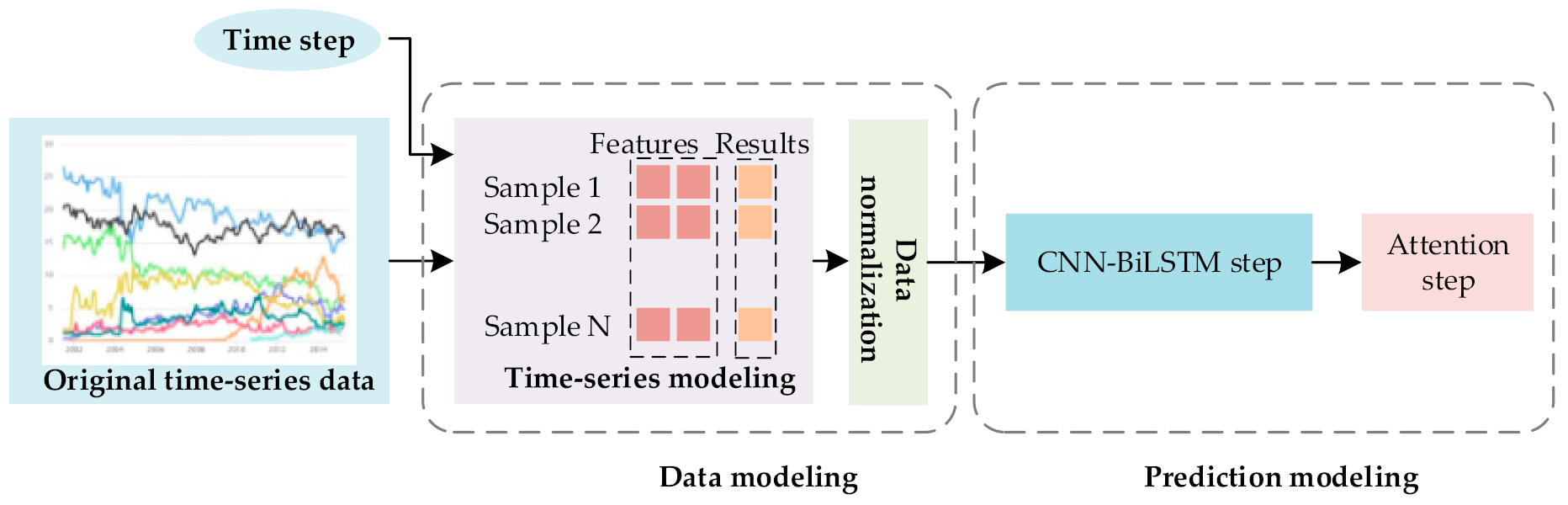
The framework of the proposed CNN-BiLSTM-Attention model for PM2.5 concentration prediction is given in Figure 1. In general, the original data is divided into a series of samples. Additionally, the feature set, related to PM2.5 concentration, meteorological data, and air quality data, are split from the samples. Their values are then normalized into the range of 0 to 1. The processed dataset is input into the model for training, after that, the trained model is used to predict the PM2.5 concentration. To sum up, the framework contains two phases, a data modeling phase and a prediction modeling phase. The specific contents of these two phases are described as follows.
2.1. Data Modeling Phase
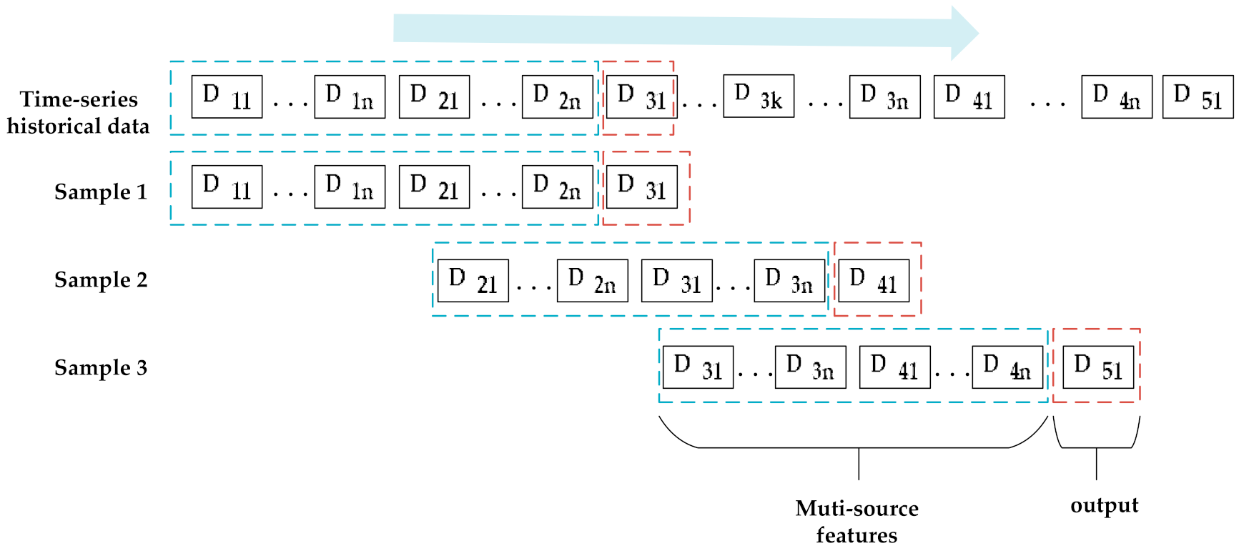
In the case of multivariate prediction, the data at time t includes meteorological data, air quality data, and PM2.5 concentration. The dataset at time tm is denoted as Dm1, …, Dmn. n represents the number of data at time tm. When the feature size is set to 2n, each sample contains 2n data. In Figure 2, sample 1 contains D11, …, D1n and D21, …, D2n, and each item represents a type in a multivariate dataset, such as PM2.5 concentration, wind speed, SO2, etc. Inputting these variables into the model will output the predicted PM2.5 concentration value, which is marked by a red box. The first item of each multivariate data, such as D11, D21, …, D51, represent the PM2.5. concentration. The same rules apply to other variables.
2.2. Prediction Modeling Phase
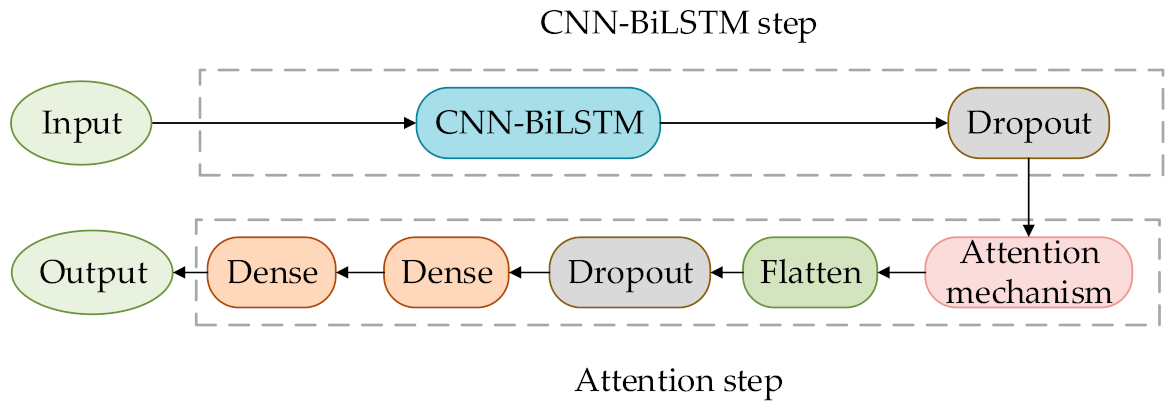
The prediction modeling phase is divided into two steps, as shown in Figure 3. One is CNN-BiLSTM, and the other is attention. During the process of CNN-BiLSTM, the training set mentioned above are first used as the input of CNN. Those features that are related to PM2.5 concentration and extracted by CNN are input into BiLSTM. Then, the dropout is used to process the output of BiLSTM, and the output of the dropout is considered the output of the CNN-BiLSTM step. Meanwhile, the output of CNN-BiLSTM step is entered into the Attention step. Specifically, the output of the dropout is entered into the attention mechanism, followed by a flatten layer, dropout layer, and two dense layers for training the proposed model. Finally, the results of PM2.5 concentration prediction are obtained when the test set is input into the proposed model.
In the following section, the CNN-BiLSTM and the attention mechanism of the prediction modeling phase are described in detail.
2.2.1. CNN-BiLSTM
It is very reasonable to use 1D convolution to extract features of one-dimensional time series such as PM2.5 concentration. In the CNN layer, the rectified linear unit (relu) function, given in Equation (1), is used as an activation function, which can avoid neuron death by modifying the negative value and solve the gradient vanishing and exploding problems [25]. Additionally, the input matrix of each training set is 720*13. The 720 is obtained by multiplying 24 by 30, where 24 means that a day contains 24 samples in total, and 30 means that a total of 30 days of samples are entered. Additionally, the 13 is the number of variables included in each sample. After extracting features through the CNN layer, the shape of the output matrix is reduced to 720*12. In the BiLSTM layer, the output of CNN is input into BiLSTM, and the generated shape is 720*8.
2.2.2. Attention Mechanism
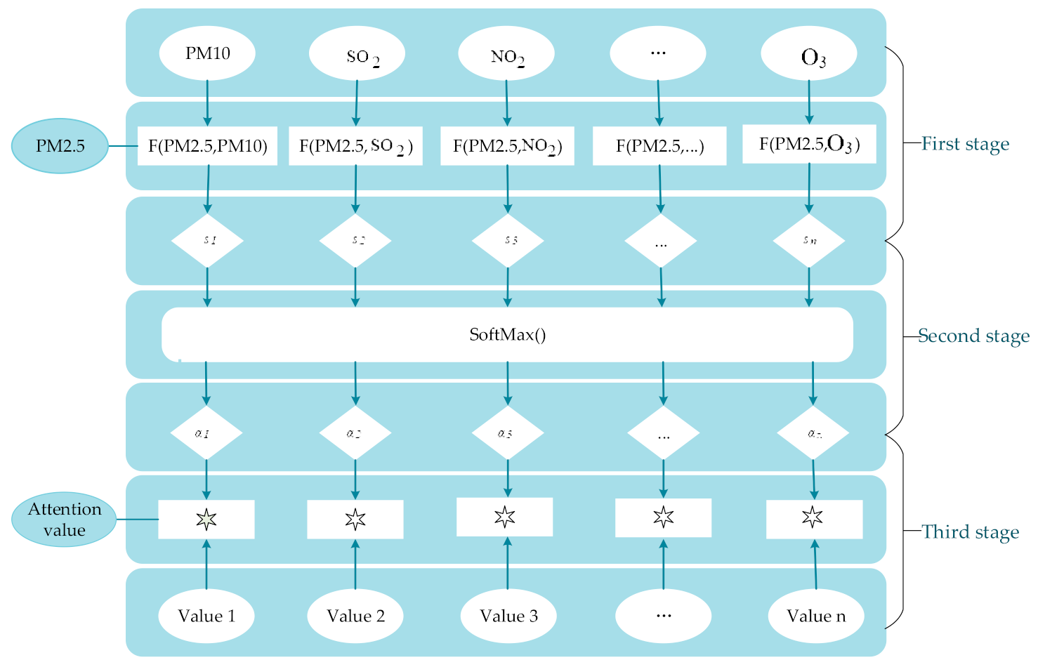
The main idea of the attention mechanism comes from the process of human visual attention. Human vision can quickly find key areas and add focus to them to obtain more detailed information. Based on the PM2.5 concentration prediction, it can selectively pay attention to some more important information related to PM2.5 concentration, assigns the weight for those, and ignores the irrelevant information [26].
The attention mechanism, given in Figure 4, is divided into three stages. In the first stage, the similarity score between PM2.5 concentration and other variables’ values are calculated, as shown in Equation (2). This is just one way to calculate the score, which is obtained from the current state of the neural unit itself, not the previous state. It is a highly accepted calculation method. In the second stage, the softmax function is used to normalize the similarity score obtained in the first stage to get the weight coefficient of each BiLSTM unit output vector, which can be defined as Equation (3). In the third stage, it can be seen from Equation (4) that the attention mechanism performs a weighted summation on the vector output by each BiLSTM unit and the weight coefficient obtained above to get the final attention values of each variable.
where j indicates the serial number of variables, t denotes the current moment, represents the similarity score of PM2.5 concentration to other variables, and , , and stand for weight matrix, the output of BiLSTM layer, and bias unit, respectively.
3. Experiment
In the present section, the proposed CNN-BiLSTM-Attention model is used to predict the PM2.5 concentration in Beijing.
3.1. Dataset and Preprocessing
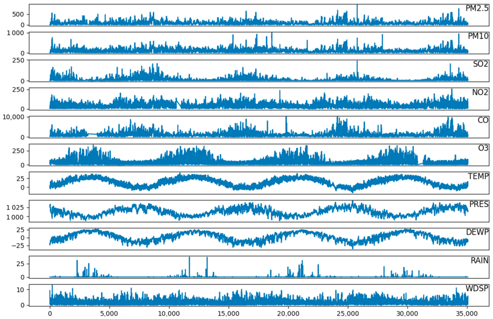
The dataset consists of 35,064 climate and pollution records from between January 2013 and February 2017 in Shunyi District. It covers 13 variables given in Table 1, including PM2.5 concentration, PM10, SO2, NO2, CO, O3, temperature (TEMP), air pressure (PRES), dew point temperature (DEWP), rainfall (RAIN), wind speed (WDSP), year, and month. Meanwhile, the mean interpolation is adopted to fill in the missing values of the dataset for improving its data quality. Variables of the dataset are given in Figure 5.
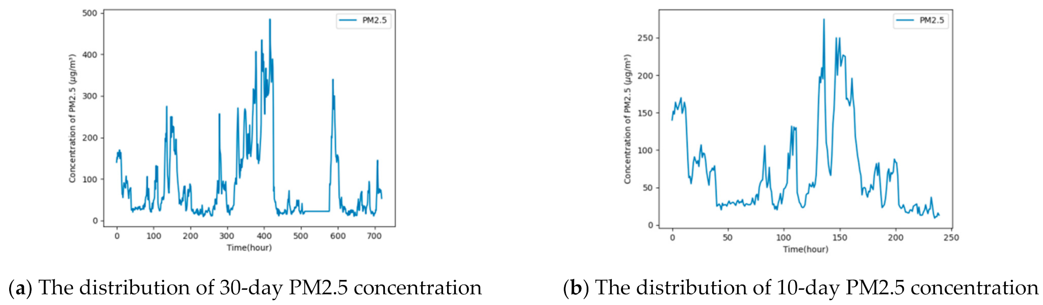
The horizontal ordinate in Figure 5 represents the time in hours from 1 January 2013 to 28 February 2017, and the longitudinal coordinate represent the value of each variable. It can be seen clearly that these variables have obvious periodicity. Therefore, year and month are also chosen as features for achieving higher accurate prediction of PM2.5 concentration. To further determine the period, the distribution of PM2.5 concentration for 30-day and 10-day are displayed. It can be seen from Figure 6 that there are three obvious peaks in the 30-day PM2.5 concentration distribution, and there is one peak in the 10-day graph, so 10 days are determined as a cycle.
Since the variables used in predicting the PM2.5 concentration have different dimensions, the value of PM2.5 concentration ranges from 2 to 900, and the value of WDSP ranges from 0 to 13. If these data are directly used as the input of the neural network, large deviations will affect the results. Therefore, the min-max method, given in Equation (5), is used to make the data more concentrated. Additionally, in the experiment, 80%, 10%, and 10% of the dataset are used as the training set, validation set, and testing set of the proposed model, respectively.
3.2. Rating Indicators and Experimental Settings
Mean absolute error (MAE), root mean square error (RMSE), and R2 are commonly used indicators to measure the accuracy of prediction, and they are also important scales for evaluating models in deep learning. Therefore, the three indicators are used for comparing the performance of the models, and they are defined as Equations (6)–(8).
where N, Pi, and Oi represent the number of a dataset, predicted values, and observed values of PM2.5 concentration, respectively. The smaller value of MAE and RMSE means that the smaller error between the predicted value and the observed value of PM2.5 concentration, the higher accuracy of the prediction model. Additionally, the value of R2 stands for the matching degree between these two values, the closer R2 is to 1, the better the prediction performance of the model, and the closer to 0 the lower the prediction accuracy.
The proposed model is implemented by the computer with AMD Ryzen 7 3800X 8-core Processor CPU, NVIDIA GeForce RTX 2060 SUPER, and 16G running memory, using the TensorFlow neural network framework. The details of the hyperparameter used in the experiment are shown in Table 2. The step size of the convolution kernel is 1, and the Glorot uniform initializer is used to initialize the weights of the neural network. The initial value of the bias unit is set to 0.
For the time series model, the size of input and output variables are very important parameters. The oversize length of variables will increase the computational complexity, and the undersize length of variables will make the model unable to extract effective features. Owing to the strong periodicity of PM2.5 concentration and other related variables, it is determined that the period is ten days mentioned above. A large number of experiments are implemented on the CNN-BiLSTM-Attention model to obtain the appropriate size of variables for PM2.5 concentration prediction, and the results are given in Table 3. Different values of MAE and RMSE indicate that when the input size is 24*30 and the output size is 48, the error reaches its lowest, whether it is MAE or RMSE. Therefore, 768 variables in each sample are used as input in the multi-source experiment.
3.3. Results and Discussion
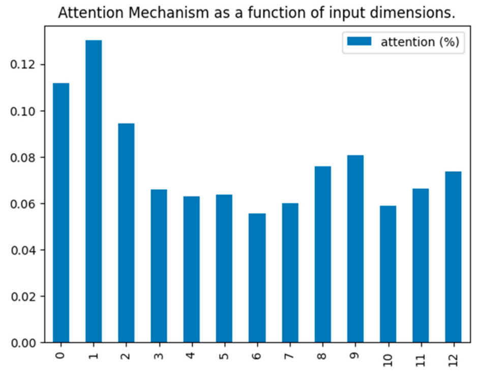
The CNN-BiLSTM-Attention model is applied to the preprocessed dataset mentioned above to predict the PM2.5 concentration. Additionally, the attention values on each variable are obtained. The result is shown in Figure 7, where 0–12 on the horizontal ordinate represent PM2.5, PM10, SO2, NO2, CO, O3, TEMP, PRES, DEWP, RAIN, WDSP, year, and month, and longitudinal coordinate indicates the attention value, showing the importance of each variable in the process of predicting PM2.5 concentration. The weights assigned to each variable are 0.131, 0.101, 0.077, 0.088, 0.073, 0.066, 0.065, 0.05, 0.053, 0.051, 0.059, 0.083, and 0.095. Among them, PM2.5 and PM10 have gained relatively large weights because they have a greater impact on the PM2.5 concentration.
3.3.1. Short-Term Forecast with Multi-Source Data
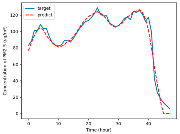
In order to verify the performance of the proposed model, we first start with short-term predictions. A piece of input data is randomly selected from the test set. Figure 8 compares the prediction results of the proposed model (marked with a red dotted line) with original PM2.5 concentrations (marked with a blue solid line). It can be seen that although the PM2.5 concentration value fluctuates greatly, the proposed model can still fit perfectly. Additionally, the performance index MAE, RMSE, and R2 are 1.3, 1.702, and 0.978, respectively.
To ensure the generalization of the proposed model, 10 sets of test sets were randomly selected for experiments, and MAE, RMSE, and R2 are shown in Table 4. The average values of MAE, RMSE, and R2 of the 10 experiments are calculated, which are 2.366, 3.095, and 0.960, respectively.
Furthermore, comparison models are set up to verify the superiority of the proposed model. The performance of the traditional models, machine learning models, and the deep learning models, such as Lasso Regression, Ridge Regression, XGBOOST, SVR, CNN-LSTM, CNN-BiLSTM, and CNN-BiLSTM-Attention model are compared by experimenting on the hourly dataset of Beijing Shunyi District. The parameters of all the comparison models are adjusted to their optimal values.
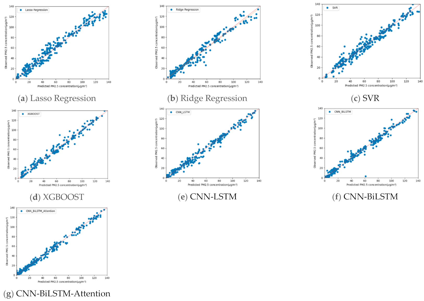
Figure 9 shows the scatter dots of the predicted values of the PM2.5 concentration drawn by the comparison model and the proposed model. The closer the scatter dots are to the diagonal line, the smaller the error is between the predicted and the observed values. It can be intuitively seen from the figure that the performance of the machine learning models is greater than the traditional models, but the prediction result of SVR is poor. Additionally, the precision of deep learning models is better than the machine learning models. The reason for this phenomenon is that the traditional regression method and the two machine learning algorithms used to predict PM2.5 concentration have linear characteristics. However, in reality there is a non-linear relationship between the PM2.5 concentration and the factors related to it. However, among the CNN-LSTM model, CNN-BiLSTM model, and CNN-BiLSTM-Attention model, the performance of the three models shown in Figure 10 is almost the same.
A more accurate comparison of the three deep learning models mentioned above is performed below. As shown in Figure 10, it is not difficult to find that the performance of the proposed model is better than the other two in terms of convergence speed. It can be seen that when the epoch is almost 20, the loss value of the CNN-BiLSTM-Attention model is already lower than the other two models.
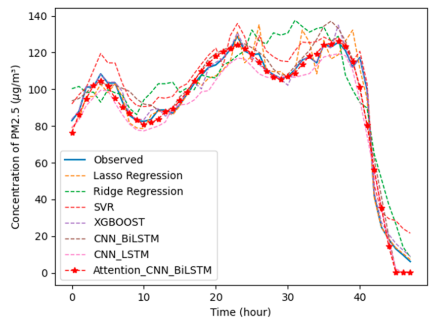
To further compare the prediction effects of the proposed method and other comparative model methods, Figure 11 shows the predicted values of each model and the actual observed PM2.5 value of the test set. The x-axis in the figure represents the time stamp, and the y-axis represents the PM2.5 concentration. On the left is the color bar, and the blue line represents the actual observation value. Similar to Figure 9, our proposed model with the red star-shaped line is still closest to the real data and is better than the other two deep learning models, represented by a red dashed line and a brown dashed line, respectively.
The quantitative performance of the proposed model and those used as comparison models are summarized in Table 5. For the proposed model, the prediction results that are denoted in bold are significantly improved compared to the other six models, achieving the best indicator values (MAE: 2.366 , RMSE: 3.095 , R2: 0.960). The main reason is that this model can not only handle the characteristics of non-linear relationships, but the attention mechanism can mine better feature information. Therefore, compared with other comparison models, the proposed model has a competitive advantage when predicting PM2.5 concentrations.
3.3.2. Long-Term Forecast with Multi-Source Data
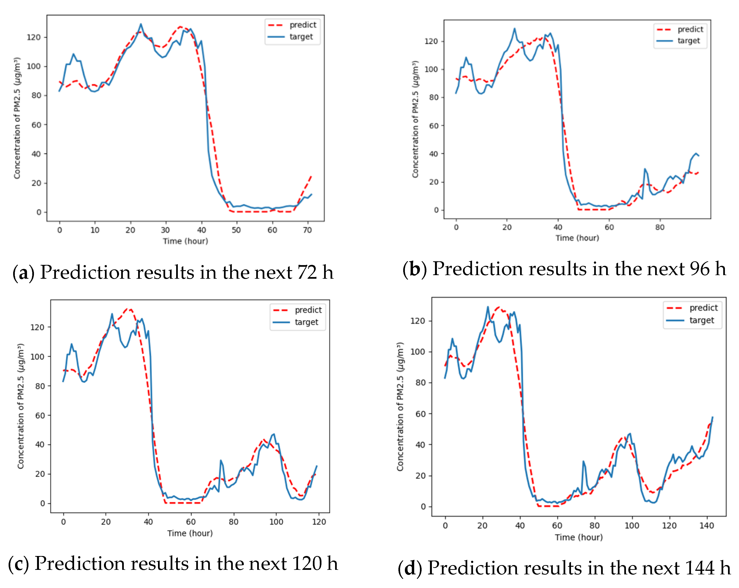
In addition, a long-term PM2.5 concentration prediction is carried out to fully reflect the robustness of the proposed model, such as 72 h, 96 h, 120 h, and 144 h. Figure 12 indicates that when the PM2.5 concentration value fluctuates greatly, the proposed model can still track the general trend very well, but the deviation will be relatively large in small fluctuations. This can be attributed to a long time of prediction. The longer the time, the correlation between the features extracted by the model and the PM2.5 concentration will decrease, and the prediction error will increase.
In order to show the superiority of the proposed model for predicting PM2.5 concentration in more detail, long-term predictions have also been made for all comparative models. The MAE and RMSE are still used as evaluation indicators. The results are shown in Table 6 and Table 7. When predicting the PM2.5 concentration in the next 24 h, although CNN-LSTM is smaller than CNN-BiLSTM-Attention on MAE, it is larger than CNN-BiLSTM-Attention on RMSE. Additionally, the CNN-BiLSTM-Attention model is optimal at 48 h, whether on MAE or RMSE. As the prediction time increases, the relevance of the data decreases, and the influence of other variables on the current PM2.5 concentration is reduced, the weight of important features extracted by attention is also affected. Therefore, the prediction accuracy will decrease. However, the proposed model still performs better than the other six models, which can be seen from Table 6. Even if the proposed model is used to predict the next 144 h, it is more accurate than machine learning at predicting the next 48 h. Therefore, this model can solve the problem of long term PM2.5 concentration prediction.
Based on the above results, we summarize this study as follows:
- (1)
- Firstly, we obtain multi-source data that are composed of PM2.5 concentration values, meteorological data, and air quality data in hourly units and sourced from the U.S. Embassy in Beijing. There are missing values in the dataset due to uncontrollable factors, which we use mean interpolation to fill in, and the min-max method is used to normalize the data to make the model more stable.
- (2)
- Secondly, the role of hyperparameters in a model is very important. We determine the values of the hyperparameters through parameter tuning tools and experimental results, and then ensure the input and output feature sizes through a large number of experiments.
- (3)
- Finally, the proposed model is used to predict the PM2.5 concentration. To prove the better performance of the proposed model, six comparison models are set up. Additionally, we verify the effectiveness of the model from both short-term and long-term aspects. In terms of short-term forecasts, the results show that the proposed model not only has a smaller error, but also holds a faster convergence speed. In terms of long-term forecasts, although the error value of prediction will become larger and larger, the results are also better than other comparison models.
4. Conclusions
In recent years, predicting the PM2.5 concentration has attracted the attention of many scholars, especially those who are committed to environmental protection. Coupled with the improvement of urban air pollution prediction and control management, many air quality monitoring stations are deployed in many cities. How to effectively use the data collected by these monitoring stations and improve urban air quality is an important issue. In this paper, an intelligent PM2.5 concentration prediction model CNN-BiLSTM-Attention is proposed.
Taking Beijing as a research case, this model was applied to a dataset of hours from January 2013 to February 2017 in Shunyi District, Beijing. Results show that:
- (1)
- For a model based on deep learning, the parameters adjustment of the network framework is inevitable. In this paper, a large number of experiments and tuning tools are used to determine the parameters.
- (2)
- The performance of the hybrid CNN-BiLSTM-Attention model proposed in this paper is better than the traditional models and machine learning models used to predict PM2.5 concentration. Additionally, it is better than the integration of the two models based on CNN and LSTM. This is due to the attention mechanism that can capture the degree of influence of the feature states at different times on the PM2.5 concentration. The attention-based layer can automatically weight the past feature states.
- (3)
- The short-term (48 h) and long-term (72 h, 96 h, 120 h, and 144 h) predictions of the models carried out in this paper show that the prediction performance is the best in the next 48 h, with MAE, RMAE and R2 being 2.366 , 3.065 and 0.960, respectively. Additionally, the CNN-BiLSTM-Attention model predicts the next 144 h is still better than other models’ predictions for the next 48 h. Therefore, this hybrid model has good generalization ability and is also conducive to long-term dependence feature extraction.
The proposed CNN-BiLSTM-Attention model is an intelligent PM2.5 concentration prediction model based on the analysis and modeling of historical air quality data. It can help environmental protection agencies implement some measures to strengthen environmental protection. Meanwhile, it provides a reference for the measures taken by the transportation-related departments to reduce related gas emissions. The model established in this paper is closely related to reality, deeply analyzes and discusses PM2.5 issues, establishes a corresponding model, and analyzes the prediction accuracy so that the model has good versatility and generalization. It can also be used to predict other pollutants. With the large-scale deployment of air quality monitoring stations, the prediction model in this paper has potential for application.
However, since air quality monitoring stations have only been deployed in recent years, the limitation of the amount of data may affect the training of the model. In the future, as more air quality monitoring stations are deployed, there will be longer periods of data to optimize the prediction model. In addition, the PM2.5 concentration is spatially related. In the future, PM2.5 concentration data from surrounding monitoring stations and related factors will be taken into consideration to further improve the prediction accuracy of the model.
Author Contributions
Conceptualization, J.Z. and B.R.; methodology, T.L. and Y.P.; validation, Y.P.; formal analysis, J.Z.; investigation, Y.P.; resources, Y.P.; data curation, B.R.; writing—original draft preparation, J.Z. and Y.P.; writing—review and editing, T.L. and B.R.; visualization, Y.P.; supervision, T.L. and J.Z.; project administration, T.L.; funding acquisition, J.Z. and T.L. All authors have read and agreed to the published version of the manuscript.
Funding
This research was funded by the National Natural Science Foundation of China, grant number 51939001 and 61976033, the Liaoning Revitalization Talents Program, grant number XLYC1907084, the Science & Technology Innovation Funds of Dalian, grant number 2018J11CY022 and 2018J11CY023, the China Postdoctoral Science Foundation, grant number 2016M591421, the Fundamental Research Funds for the Central Universities, grant number 3132019353, 3132019322, 3132021273 and 3132021274.
Data Availability Statement
Not applicable.
Conflicts of Interest
The authors declare no conflict of interest.
References
- Zhang, X.; Murakami, T.; Wang, J.H.; Aikawa, M. Sources, species and secondary formation of atmospheric aerosols and gaseous precursors in the suburb of Kitakyushu, Japan. Sci. Total Environ. 2021, 763, 143001. [Google Scholar] [CrossRef] [PubMed]
- Brook, R.D.; Franklin, B.; Cascio, W.; Hong, Y.L.; Howard, G.; Lipsett, M.; Luepker, R.; Mittleman, M.; Samet, J.; Smith, S.C.; et al. Air Pollution and Cardiovascular Disease: A Statement for Healthcare Professionals From the Expert Panel on Population and Prevention Science of the American Heart Association. Circulation 2004, 109, 2655–2671. [Google Scholar] [CrossRef] [PubMed]
- Wang, L.N.; Wu, X.M.; Du, J.Q.; Cao, W.N.; Sun, S. Global burden of ischemic heart disease attributable to ambient PM2.5 pollution from 1990 to 2017. Chemosphere 2021, 263, 128134. [Google Scholar] [CrossRef] [PubMed]
- Akhbarizadeh, R.; Dobaradaran, S.; Torkmahalleh, M.A.; Saeedi, R.; Aibaghi, R.; Ghasemi, F.F. Suspended fine particulate matter (PM2.5), microplastics (MPs), and polycyclic aromatic hydrocarbons (PAHs) in air: Their possible relationships and health implications. Environ. Res. 2021, 192, 110339. [Google Scholar] [CrossRef] [PubMed]
- Song, C.B.; Wu, L.; Xie, Y.C.; He, J.J.; Chen, X.; Wang, T.; Lin, Y.C.; Jin, T.S.; Wang, A.X.; Liu, Y.; et al. Air pollution in China: Status and spatiotemporal variations. Environ. Pollut. 2017, 227, 334–347. [Google Scholar] [CrossRef] [PubMed]
- Khan, M.R.; Sarkar, B. Change Point Detection for Diversely Distributed Stochastic Processes Using a Probabilistic Method. Invention 2019, 4, 42. [Google Scholar] [CrossRef] [Green Version]
- Khan, M.R.; Sarkar, B. Change Point Detection for Airborne Particulate Matter (PM2.5, PM10) by Using the Bayesian Approach. Mathematics 2019, 7, 474. [Google Scholar] [CrossRef] [Green Version]
- Woody, M.C.; Wong, H.W.; West, J.J. Arunachalam, S. Multiscale predictions of aviation-attributable PM 2.5 for U.S. airports modeled using CMAQ with plume-in-grid and an aircraft-specific 1-D emission model. Atmos. Environ. 2016, 147, 384–394. [Google Scholar] [CrossRef]
- Geng, G.N.; Zhang, Q.; Martin, R.V.; Donkelaar, A.V.; Huo, H.; Che, H.Z.; Lin, J.T.; He, K.B. Estimating long-term PM 2.5 concentrations in China using satellite-based aerosol optical depth and a chemical transport model. Remote Sens. Environ. 2015, 166, 262–270. [Google Scholar] [CrossRef]
- Dong, M.; Yang, D.; Kuang, Y.; He, D.; Erdal, S.; Kenski, D. PM 2.5 concentration prediction using hidden semi-Markov model-based times series data mining. Expert Syst. Appl. 2009, 369, 9046–9055. [Google Scholar] [CrossRef]
- Murillo-Escobar, J.; Sepulveda-Suescun, J.P.; Correa, M.A.; Orrego-Metaute, D. Forecasting concentrations of air pollutants using support vector regression improved with particle swarm optimization: Case study in Aburrá Valley, Colombia. Urban Clim. 2019, 29, 100473. [Google Scholar] [CrossRef]
- Pandey, G.; Zhang, B.; Jian, L. Predicting submicron air pollution indicators: A machine learning approach. Environ. Sci. Process. Impacts 2013, 15, 996–1005. [Google Scholar] [CrossRef]
- Hopfield, J.J. Neural Networks and Physical Systems with Emergent Collective Computational Abilities. Proc. Natl. Acad. Sci. USA 1982, 79, 2554–2558. [Google Scholar] [CrossRef] [Green Version]
- Hochreiter, S.; Schmidhuber, J. Long Short-Term Memory. Neural Comput. 1997, 9, 1735–1780. [Google Scholar] [CrossRef] [PubMed]
- Lagesse, B.; Wang, S.Q.; Larson, T.V.; Kim, A. Predicting PM2.5 in Well-Mixed Indoor Air for a Large Office Building Using Regression and Artificial Neural Network Models. Environ. Sci. Technol. 2020, 54, 15320–15328. [Google Scholar] [CrossRef]
- Graves, A.; Schmidhuber, J. Framewise phoneme classification with bidirectional LSTM and other neural network architectures. Neural Netw. 2005, 18, 602–610. [Google Scholar] [CrossRef] [PubMed]
- Li, W.J.; Qi, F.; Tang, M.; Yu, Z.T. Bidirectional LSTM with self-attention mechanism and multi-channel features for sentiment classification. Neurocomputing 2020, 387, 63–77. [Google Scholar] [CrossRef]
- Rathor, S.; Agrawal, S. A robust model for domain recognition of acoustic communication using Bidirectional LSTM and deep neural network. Neural Comput. Appl. 2021, 1–10, in press. [Google Scholar]
- Liu, H.; Duan, Z.; Chen, C. A hybrid multi-resolution multi-objective ensemble model and its application for forecasting of daily PM2.5 concentrations. Inf. Sci. 2020, 516, 266–292. [Google Scholar] [CrossRef]
- Alkhodari, M.; Fraiwan, L. Convolutional and recurrent neural networks for the detection of valvular heart diseases in phonocardiogram recordings. Comput. Methods Programs Biomed. 2021, 200, 105940. [Google Scholar] [CrossRef]
- Guan, Z.Y.; Xing, Q.L.; Xu, M.; Yang, R.; Liu, T.; Wang, Z.L. MFQE 2.0: A New Approach for Multi-frame Quality Enhancement on Compressed Video. IEEE Trans. Pattern Anal. Mach. Intell. 2021, 43, 949–963. [Google Scholar] [CrossRef] [Green Version]
- Aslan, M.F.; Unlersen, M.F.; Sabanci, K.; Durdu, A. CNN-based transfer learning–BiLSTM network: A novel approach for COVID-19 infection detection. Appl. Soft Comput. 2021, 98, 106912. [Google Scholar] [CrossRef]
- Zhu, J.Q.; Deng, F.; Zhao, J.C.; Zheng, H. Attention-based parallel network (APNet) for PM2.5 spatiotemporal prediction. Sci. Total Environ. 2021, 769, 145082. [Google Scholar] [CrossRef]
- Zhang, B.; Zhang, H.W.; Zhao, G.M.; Lian, J. Constructing a PM 2.5 concentration prediction model by combining auto-encoder with Bi-LSTM neural networks. Environ. Model. Softw. 2020, 124, 104600. [Google Scholar] [CrossRef]
- Yang, Z.B.; Zhang, J.P.; Zhao, Z.B.; Zhai, Z.; Chen, X.F. Interpreting network knowledge with attention mechanism for bearing fault diagnosis. Appl. Soft Comput. 2020, 97, 106829. [Google Scholar] [CrossRef]
- Bahdanau, D.; Cho, K.H.; Bengio, Y. Neural Machine Translation by Jointly Learning to Align and Translate. In Proceedings of the 3rd International Conference on Learning Representations (ICLR2015), San Diego, CA, USA, 7–9 May 2015. [Google Scholar]
Figure 1.
The framework of CNN-BiLSTM-Attention.

Figure 2.
Examples of data modeling.

Figure 3.
The steps of prediction modeling.

Figure 4.
The process of the attention mechanism.

Figure 5.
Distribution of different variables.

Figure 6.
The trend of PM2.5 concentration.

Figure 7.
The attention values of the input variables.

Figure 8.
Results of PM2.5 concentration prediction using the CNN-BiLSTM-Attention model.

Figure 9.
Comparisons of the observed and predicted values of PM2.5 concentration values.

Figure 10.
Comparisons of convergence speed in three deep learning models.

Figure 11.
Comparisons of predicted and observed values of each model.

Figure 12.
Long-term prediction of PM2.5 concentration by CNN-BiLSTM-Attention model.


Table 1.
Variables contained in the dataset.
| Categories | Input Variables | Unit |
|---|---|---|
| Pollutant | PM2.5 | |
| Climate Variables | PM10 | |
| mg/m3 | ||
| mg/m3 | ||
| CO | mg/m3 | |
| O3 | mg/m3 | |
| TEMP | °C | |
| PRES | KPa | |
| DEWP | °C | |
| RAIN | mm | |
| WDSP | km/h | |
| Time Variables | Year | - |
| Month | - |
Table 2.
Hyperparameters of CNN-BiLSTM-Attention model.
| Hyperparameter | Value |
|---|---|
| Filter size for CNN | 12 |
| Kernel size for CNN | 64 |
| Padding | same |
| Activation function | relu |
| Unit number for BiLSTM | 4 |
| Dropout rate for BiLSTM | 0.2 |
| Dropout rate for Flatten | 0.5 |
| Neuron number for Attention | 720 |
| Optimization function | Adam |
| Learning-rate | 0.001 |
| Batch size | 150 |
| Epoch number | 50 |
Table 3.
MAE and RMSE with different input and output variable values (Unit: ).
| Input | Output | |||||
|---|---|---|---|---|---|---|
| 24 h | 48 h | 72 h | ||||
| MAE | RMSE | MAE | RMSE | MAE | RMSE | |
| 24*10 h | 5.604 | 6.268 | 5.946 | 5.202 | 5.969 | 6.290 |
| 24*20 h | 4.829 | 5.740 | 4.986 | 6.043 | 3.928 | 5.715 |
| 24*30 h | 4.228 | 5.295 | 2.366 | 3.095 | 3.777 | 4.834 |
| 24*40 h | 4.468 | 5.694 | 3.872 | 3.988 | 4.239 | 6.876 |
Table 4.
The MAE, RMSE (Unit: ), and R2 of the 10 randomized trials of the proposed model.
| Sample | MAE | RMSE | R2 |
|---|---|---|---|
| 1 | 3.034 | 4.099 | 0.947 |
| 2 | 2.569 | 3.527 | 0.951 |
| 3 | 2.006 | 2.991 | 0.963 |
| 4 | 2.606 | 3.480 | 0.955 |
| 5 | 2.001 | 2.531 | 0.962 |
| 6 | 5.821 | 7.503 | 0.934 |
| 7 | 1.878 | 2.033 | 0.958 |
| 8 | 1.725 | 2.122 | 0.965 |
| 9 | 0.718 | 0.964 | 0.982 |
| 10 | 1.300 | 1.702 | 0.978 |
| Avg | 2.366 | 3.095 | 0.960 |
Table 5.
MAE, RMSE (Unit: ), and R2 of the proposed model and the comparison model.
| Models | MAE | RMSE | R2 |
|---|---|---|---|
| CNN-BiLSTM-Attention | 2.366 | 3.095 | 0.960 |
| CNN-BiLSTM | 3.851 | 5.333 | 0.912 |
| CNN-LSTM | 5.577 | 7.032 | 0.906 |
| XGBOOST | 7.607 | 8.541 | 0.890 |
| SVR | 7.796 | 8.549 | 0.858 |
| Ridge Regression | 7.695 | 9.032 | 0.878 |
| Lasso Regression | 7.845 | 9.781 | 0.844 |
Table 6.
MAE for long-term prediction of each model (Unit: ).
| Models | 24 | 48 | 72 | 96 | 120 | 144 |
|---|---|---|---|---|---|---|
| CNN-BiLSTM-Attention | 4.228 | 2.366 | 3.777 | 6.036 | 6.337 | 6.918 |
| CNN-BiLSTM | 4.437 | 3.851 | 5.652 | 6.788 | 6.797 | 7.452 |
| CNN-LSTM | 3.837 | 5.577 | 7.234 | 7.671 | 9.148 | 12.384 |
| XGBOOST | 5.275 | 7.607 | 7.928 | 10.554 | 12.744 | 13.318 |
| SVR | 7.762 | 7.796 | 10.486 | 11.102 | 11.405 | 11.834 |
| Ridge Regression | 7.832 | 7.695 | 11.502 | 12.364 | 13.649 | 14.823 |
| Lasso Regression | 7.845 | 7.845 | 11.464 | 11.775 | 12.779 | 13.914 |
Table 7.
RMAE for long-term prediction of each model (Unit: ).
| Models | 24 | 48 | 72 | 96 | 120 | 144 |
|---|---|---|---|---|---|---|
| CNN-BiLSTM-Attention | 5.295 | 3.095 | 4.834 | 6.467 | 8.768 | 8.974 |
| CNN-BiLSTM | 6.215 | 5.333 | 8.219 | 7.704 | 9.063 | 10.579 |
| CNN-LSTM | 5.817 | 7.032 | 10.000 | 10.185 | 10.671 | 13.169 |
| XGBOOST | 6.041 | 8.541 | 13.290 | 15.346 | 16.800 | 16.714 |
| SVR | 8.123 | 8.549 | 11.484 | 11.945 | 12.154 | 12.884 |
| Ridge Regression | 7.961 | 9.032 | 12.722 | 13.852 | 14.254 | 15.482 |
| Lasso Regression | 8.234 | 9.781 | 12.633 | 12.975 | 13.551 | 16.394 |
Publisher’s Note: MDPI stays neutral with regard to jurisdictional claims in published maps and institutional affiliations. |
© 2021 by the authors. Licensee MDPI, Basel, Switzerland. This article is an open access article distributed under the terms and conditions of the Creative Commons Attribution (CC BY) license (https://creativecommons.org/licenses/by/4.0/).
Share and Cite
MDPI and ACS Style
Zhang, J.; Peng, Y.; Ren, B.; Li, T. PM2.5 Concentration Prediction Based on CNN-BiLSTM and Attention Mechanism. Algorithms 2021, 14, 208. https://0-doi-org.brum.beds.ac.uk/10.3390/a14070208
AMA Style
Zhang J, Peng Y, Ren B, Li T. PM2.5 Concentration Prediction Based on CNN-BiLSTM and Attention Mechanism. Algorithms. 2021; 14(7):208. https://0-doi-org.brum.beds.ac.uk/10.3390/a14070208
Chicago/Turabian StyleZhang, Jinsong, Yongtao Peng, Bo Ren, and Taoying Li. 2021. "PM2.5 Concentration Prediction Based on CNN-BiLSTM and Attention Mechanism" Algorithms 14, no. 7: 208. https://0-doi-org.brum.beds.ac.uk/10.3390/a14070208
Note that from the first issue of 2016, this journal uses article numbers instead of page numbers. See further details here.