Article

An Integrated Deep Learning and Belief Rule-Based Expert System for Visual Sentiment Analysis under Uncertainty

by
Sharif Noor Zisad
1,
Etu Chowdhury
1,
Mohammad Shahadat Hossain
1,
Raihan Ul Islam
2 and
Karl Andersson
2,*
1
Department of Computer Science and Engineering, University of Chittagong, Chittagong 4331, Bangladesh
2
Department of Computer Science, Electrical and Space Engineering, Luleå University of Technology, 971 87 Skellefteå, Sweden
*
Author to whom correspondence should be addressed.
Submission received: 2 May 2021 / Revised: 12 July 2021 / Accepted: 13 July 2021 / Published: 15 July 2021
(This article belongs to the Special Issue New Algorithms for Visual Data Mining)

Abstract

:
Visual sentiment analysis has become more popular than textual ones in various domains for decision-making purposes. On account of this, we develop a visual sentiment analysis system, which can classify image expression. The system classifies images by taking into account six different expressions such as anger, joy, love, surprise, fear, and sadness. In our study, we propose an expert system by integrating a Deep Learning method with a Belief Rule Base (known as the BRB-DL approach) to assess an image’s overall sentiment under uncertainty. This BRB-DL approach includes both the data-driven and knowledge-driven techniques to determine the overall sentiment. Our integrated expert system outperforms the state-of-the-art methods of visual sentiment analysis with promising results. The integrated system can classify images with 86% accuracy. The system can be beneficial to understand the emotional tendency and psychological state of an individual.

1. Introduction

In the modern communication system, people use different social media platforms (e.g., Facebook, Twitter, Instagram, and Flickr) to express their opinions on various issues and activities of their daily life. In these platforms, users can share visual content with the textual one to communicate with others. It is easier to express emotions intuitively through images [1]. There is a percept that “A picture is worth a thousand words”. From Figure 1, we can understand how an image can be able to deduce an individual’s sentiment without any text. In Figure 1a, the cat is in a happy mood as it is enjoying the fruit. On the other hand, Figure 1b represents the storm forecast. Thus, visual sentiment analysis has become a part of our daily lives [2].
The accurate prediction of users’ sentiment by using their uploaded images on social media has become an important research challenge [3,4]. However, the image data may contain inconsistent data, missing data, or duplicated data which leads to various types of uncertainty (e.g., ignorance, incompleteness, imprecision, ambiguity, and vagueness). These uncertainties can obstruct prediction accuracy. For image classification, deep learning methods are widely used as they can represent the accurate and robust features of images [5,6]. In addition, to handle different types of uncertainty in image data, the Belief Rule-Based Expert System (BRBES) is more applicable  [7,8]. Since an integrated model performs better than a stand-alone model [9,10,11], we propose the integration of a deep learning method with BRBES to improve the prediction accuracy in visual sentiment analysis. This is the key contribution of our research work.
As a Deep Learning method can process raw data directly, it is used effectively to solve various classification and regression problems. However, as a data-driven approach, it has the limitation of addressing different types of uncertainty [12]. On the contrary, as a knowledge-driven approach, BRBES can address various types of uncertainty (e.g., ignorance, incompleteness, imprecision, ambiguity, and vagueness) [13]. However, it cannot integrate the associative memory in its inference procedure. For example, we use multiplication and division operators to calculate the activation weight of a rule in the BRBES inference framework. However, these provide incorrect activation values of each rule. To solve this issue, a Deep Neural Network (DNN) model can be used to calculate the rule activation weight by providing more accurate values. Therefore, as an integrated framework of the Deep Learning method within the BRBES inference framework, our proposed system provides the exact value of rule activation weights that results in an accurate prediction of sentiment under uncertainty.
BRBES is composed of a set of rules and provides results based on those rules. The rules consist of the antecedent and consequent parts. The antecedent part of a rule is based on the input, and the consequent part contains the output. Generally, there are two types of BRBES: one is Conjunctive BRB [14] and another is Disjunctive BRB [15]. The AND logical operator is utilized to connect each antecedent attribute in the Conjunctive BRB, where the OR logical operator is used in the Disjunctive one. For the AND logical operator, Conjunctive BRB takes more time in computation and constitutes a large number of rules in the rule base. In our experiments, we use the Disjunctive one as it needs less time for computation and has a low number of rules. We explore a total of eight belief rule base for BRBES that takes less computational time.
In this paper, we address the following research questions: (1) Why we use the Deep Learning model for visual sentiment analysis? (2) What is the advantage of utilizing BRBES in our proposed system? (3) Why and how we combine Deep Learning with BRBES? We compose the remainder of this paper as follows: Section 2 surveys related work on visual sentiment analysis. Section 3 provides an overview of our proposed BRB-DL approach. Section 4 discusses the procedure of experiments. Section 5 reports the experimental results and evaluation of BRB-DL compared to different models such as SVM, Naive Bias Classifier, Decision Tree classifier, VGG16, VGG19, and ResNet50. Finally, Section 6 concludes the paper with some future plans.

2. Related Work

This section presents a literature review on visual sentiment analysis. Siersdorfer and Hare [16] mainly focused on the bag-of-visual word representation and color distribution of images. They estimated the polarity of sentiment in images by extracting the discriminative sentiment-related features and deployed a machine learning approach. Machajdik and Hanbury [17] considered a method that extracted and combined low-level features of images. These features were used for emotion classification. They considered awe, amusement, contentment, excitement as positive emotions and anger, fear, disgust, and sadness as negative ones.
To generate a large-scale Visual Sentiment Ontology (VSO), Borth et al. [18] represented a method based on psychological theories and web mining. They proposed SentiBank that was a visual concept detector library. The research work was tested on a dataset of 807 artistic photographs depicting eight emotions, including amusement, awe, contentment, excitement, anger, disgust, fear, and sadness. Moreover, Chen et al. [19] introduced DeepSentiBank for detecting the emotion of an image. Vasavi and Aditi [20] adopted a Deep Learning approach to predict emotions depicted in images. They conducted their experiment on a popular Flickr Image Dataset and predicted five emotions of images including love, happiness, violence, fear, and sadness.
However, there are some data available that contain various kinds of noise. To diminish the noise of large-scale image data, You et al. [5] offered a progressive CNN (PCNN) model. In addition, to reduce over-fitting in visual sentiment analysis, Islam and Zhang [4] adopted the transfer learning approach. In this study, they utilized the hyper-parameters learned from a Deep Convolutional Neural Network (DCNN). Wang et al. [21] rendered a visual sentiment analysis framework where an adjective and a noun are jointly learned by using deep neural networks. To train a visual sentiment classifier, Vadicamo et al. [22] applied the sentiment polarity of the textual contents and proposed a cross-media learning approach. In addition, Campos et al. [6] trained an AlexNet model adapted for visual sentiment prediction.
Fengjiao and Aono [23] considered a merged method where both hand-crafted and CNN features were incorporated. They employed hand-crafted features to extract the local visual information and CNN models to get the global visual information. To label emotions of painting images, Tan et al. [24] proposed a method where the painting features were considered. They developed a classification model based on VGG16 and ResNet50. Moreover, Paolanti et al. [25] analyzed the sentiment of social images related to cultural heritage and compared them among VGG16, ResNet, and Inception models. Recently, Chowdhury et al. [26] adopted the strategy of the ensemble of transfer learning models and employed three pre-trained deep CNN models including VGG16, Xception, and MobileNet. A summary of the prior research on visual sentiment analysis is shown in Table 1. None of them applied an integrated approach to Deep Learning and BRBES. However, in our proposed method, we focus on the integration of a Deep Learning method with a BRBES inference framework. Our proposed method helps to predict the sentiment of images effectively.

3. Proposed Framework

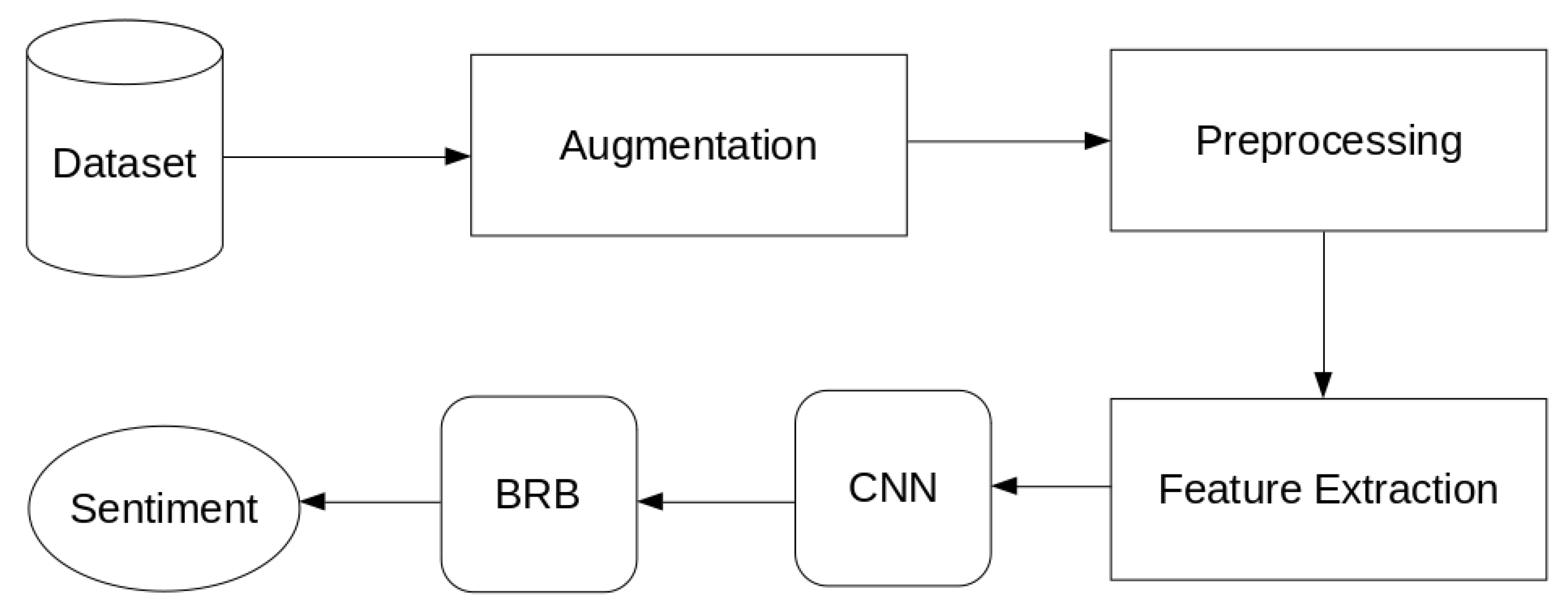
In this research, an integrated model of Convolutional Neural Network (CNN) [27] and Belief Rule Base (BRB) is developed to classify the visual sentiments. The system flow chart is illustrated in Figure 2.
From Figure 2, it can be seen that the integrated model first fetches data from the dataset and send it to the data augmentation section. After augmentation, it is sent to preprocessing steps. In the preprocessing steps, the image is resized into a 150 × 150 shape. After that, the RGB image is converted to a Gray Scale image. Then, the processed image is sent to the CNN model. The result of the CNN model is then fed into the BRB model which predicts the final sentiment label of the image.

3.1. Convolutional Neural Network Model

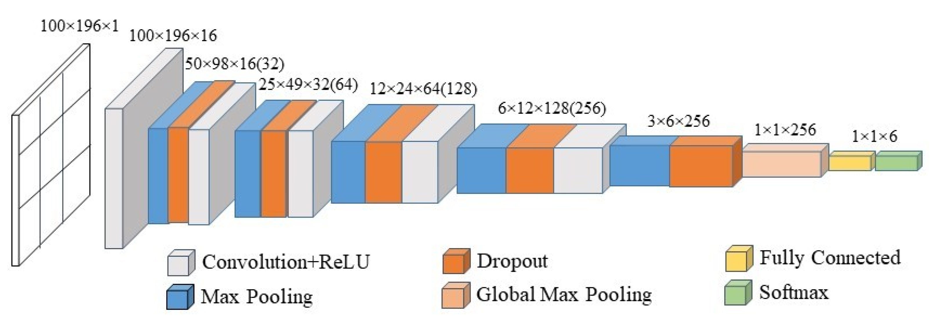
The architecture of the Convolutional Neural Network (CNN) is shown in Figure 3.
According to Figure 3, the model is constituted with five convolution layers where there are 16, 32, 64, 128, and 256 filters with 2 × 2 kernel size. ReLU activation function is used in each convolution layer. Mathematically, it can be shown as Equation (1):
R e l u ( z ) = m a x ( 0 , z ) .
The input shape of this model is (150, 150, 1), where the first 150 refers to the height of the input image and the second 150 implies the width of the input image. Finally, 1 signifies that the image is a Gray Scale image. A max pooling layer with 2 × 2 pool size is introduced in each convolution layer. The max pooling layer decreases the number of total parameters by selecting the highest value from a rectified feature map. Thus, it can lessen the data size. Along with the max pooling layer, ReLu, and dropout layer are also included in each convolution layer. ReLu works for activating the parameters while the dropout layer deactivates the neurons randomly so that it can avoid overfitting. The global Average Pooling layer is introduced in the last layer that is perfect for feeding into the dense layer. Since the model is classifying eight sentiments, the output layer has eight nodes. Therefore, Softmax is used as an activation function that can be shown as Equation (2):
s o f t m a x ( z ) = e i e i ,
Here, z is the input vector, ei is the standard exponential function of i where iz. The input vector z is the output of Fully Connected (FC) layer of the CNN model. The FC layer produces raw prediction values which are known as logits [28]. Logits are real numbers (−∞ to +∞). The softmax activation function turns these logits into the probabilities of each class.
The Adam optimizer has been used to optimize the integrated model. As a loss function, Categorical Cross-entropy is used to reduce the validation loss. The architecture of the CNN model is shown in Table 2.
The input image is an array of pixels. The convolution layer consists of multiple kernels with multiple weights. The variation of the kernel weight helps to manipulate different scales of the images. These kernels are used to extract features from the input image. The features of an image (edges, interest points, etc.) provide very rich information on the content. When a kernel is slid over the input image, it produces a feature map for different pixels. This operation is performed based on the weights of the kernel and the neighboring pixels. This feature map is then passed through the ReLu activation function, which increases the nonlinearity by converting the negative values to zero of the feature map. The pooling layer merges the features which are semantically similar into one. The max pooling layer computes the maximum value from the portion of the feature map covered by the pooling layer. For the image segmentation, the layers extract two types of features (full region feature and foreground feature) for each region. Thus, the convolution layer and the max pooling layer generate different feature maps for different images. These feature maps are used to train and validate the model.

3.2. Belief Rule-Based Expert System

A belief rule is an extended form of IF THEN rules. It consists of the antecedent part and consequent part. The antecedent part contains the antecedent attributes and the consequent part that takes the consequent attributes. Referential values are utilized by the antecedent attributes and the belief degrees are connected with the consequent attributes. The relation can be shown as Equation (3):
R k = I F ( I 1 Q 1 k ) A N D / O R ( I 2 Q 2 k ) A N D / O R . . . A N D / O R ( I T k Q T k k ) , T H E N ( O 1 , β 1 ) , ( O 2 , β 2 ) , . . . , ( O n , β n k ) ,
where I1, I2, ..., ITk are the antecedent attributes of kth rule (k = 1, 2, ..., L). Q1, Q2, ..., QTk are the referential values. O1, O2, ..., On are the referential values of the consequent attribute and β 1, β 2, ..., β n are the belief degree for each referential value, and j = 1 n β j k 1 where attribute weights are δ k 1 , δ k 2 , , δ k T k , and the rule weight is θ k .
Generally, the group of belief rules is considered as the Belief Rule Base (BRB). In a Belief Rule-Based Expert System (BRBES), it helps to generate the initial knowledge base, and Evidential Reasoning (ER) provides services as an inference engine. Some of the knowledge representation parameters are rule weight [29], belief degrees [30], and attribute weight [31]. These are used to identify uncertainty in data. The inference procedure includes input transformation [32], rule activation [29], belief update [33], and rule aggregation [34]. The working process of a BRBES is shown in Figure 4.
The process of the calculating activation weight, w k , in disjunctive BRB is shown in Equation (4):
w k = θ k i = 1 T k α i k k = 1 L ( θ k i = 1 T k α i k ) ,
where α i is the matching degree and θ k is the rule weight. The process of belief degree update is shown in Equation (5):
β i k = β ¯ i k × t = 1 T k ( τ ( t , k ) j = 1 J t α t j ) t = 1 T k ( τ ( t , k ) ) .
The original belief degree is represented by the β ¯ i k , where β i k is the updated belief degree. Rule aggregation is calculated using Equation (6):
β j = μ × k = 1 L ( w k β j k + 1 w k i = 1 N β i , k ) k = 1 L ( 1 w k i = 1 N β i , k ) 1 μ × k = 1 L ( 1 w k ) ,
μ = 1 i = 1 N k = 1 L ( w k β j k + 1 w k i = 1 N β i , k ) ( N 1 ) k = 1 L ( 1 w k i = 1 N β i , k ) ,
where β j is the ER (Evidential Reasoning) aggregated belief degree. The outputs of the rule aggregation process are some fuzzy values [7]. The process of calculating the crisp value [8] from these fuzzy outputs is shown in Equation (8):
z = i = 1 N u ( S i ) × β i ,
Here, u(Si) is the utility score for each referential value, while β i is ER aggregated belief degree. 
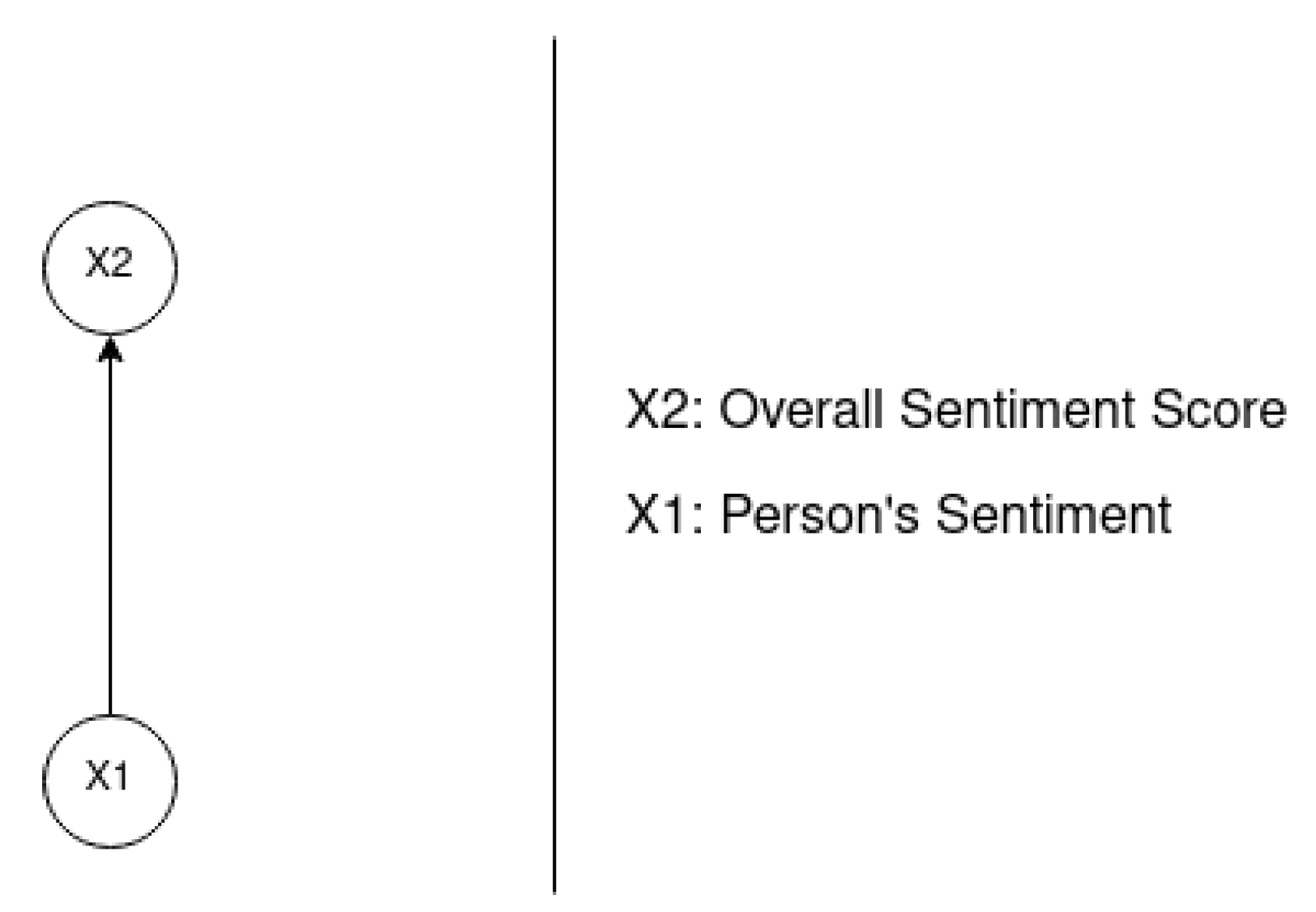
Figure 5 illustrates the Belief Rule Base Tree of our experiment. X2 which is a root node of this tree represents the “Overall Sentiment Score”. In BRB, such node is related to the consequent attribute of the rule. As mentioned earlier, this consequent attribute consists of a number of referential values, each associated with belief degree related to overall sentiment.
Considering an output from the CNN model: Anger = 0.0, Fear = 0.0, Joy = 0.0, Love = 0.0, Sadness = 0.8, and Surprise = 0.2. This output is the input ([0.0, 0.0, 0.0, 0.0, 0.8, 0.2]) for the BRB. Therefore, the matching degrees for this input are shown in Table 3.
Activation weight for this experiment is calculated with Equation (4). The rule weight ( θ k ) is considered 1 for our experiment [35]. Hence, w 1 = 1   ×   0.0 ( 1   ×   0.0 )   +   ( 1   ×   0.0 )   +   ( 1   ×   0.0 )   +   ( 1   ×   0.0 )   +   ( 1   ×   0.8 )   +   ( 1   ×   0.2 ) = 0.0 . The values of all activation weight are shown in Table 4.
Equation (5) is used to update the belief degrees. The initial belief degrees for this experiment are presented in Table 5. Since all antecedent attributes are used to define this rule base, τ ( t , k ) = 1 in this experiment [36]. Therefore, β 0 , 0 = 0.0   ×   1   ×   1   +   1   ×   1   +   1   ×   1   +   1   ×   1   +   1   ×   1   +   1   ×   1 1   +   1   +   1   +   1   +   1   +   1 = 0.0 . In the same process, we have calculated the value of β 0 , 1 to β 5 , 2 . Equations (6) and (7) are used to calculate the aggregated belief degrees. In this experiment, the calculated aggregated belief degrees for positive, neutral, and negative are shown in Table 6.

3.3. Integrated Framework

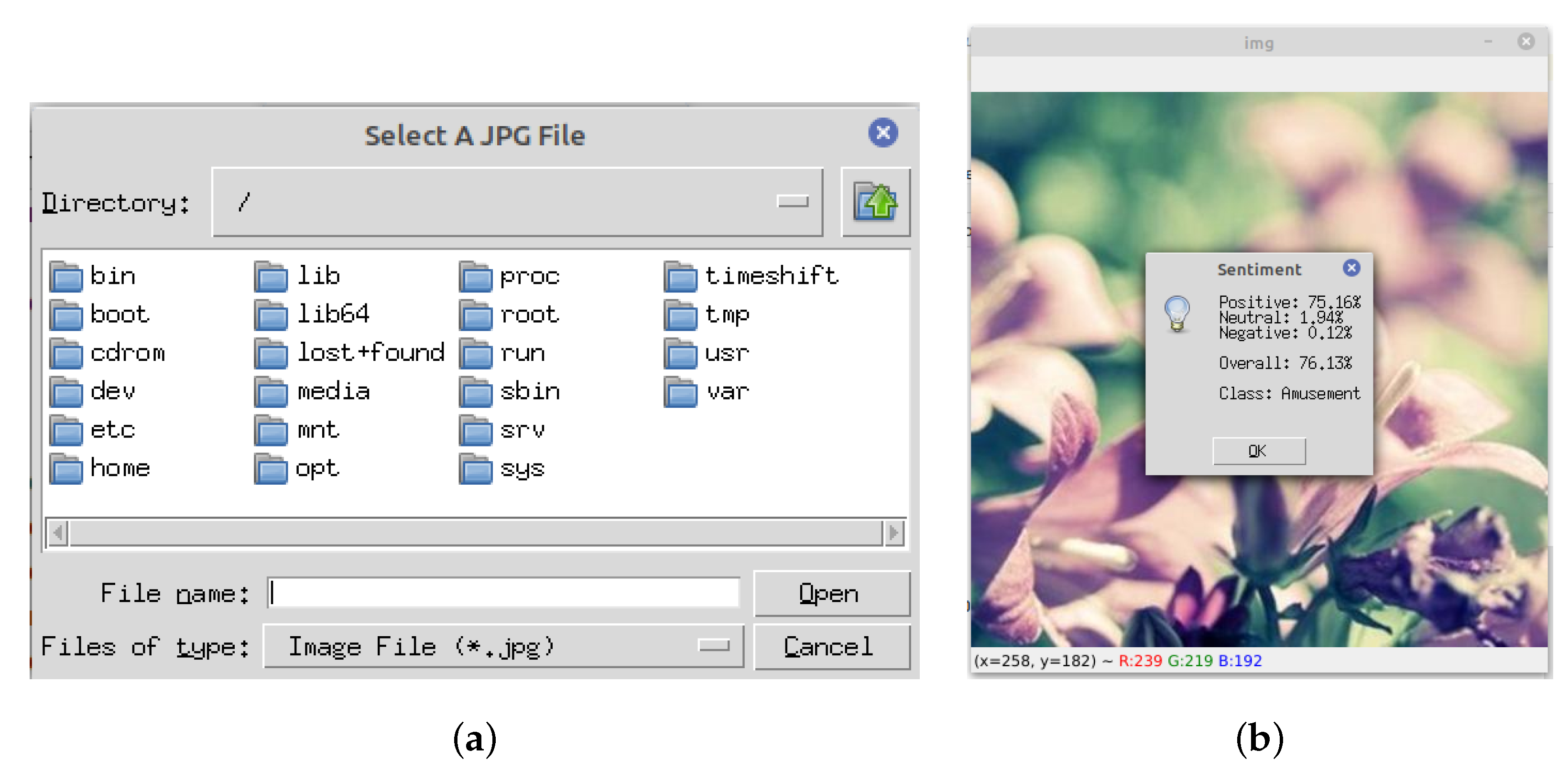
Our proposed integrated approach is used to predict the sentiment label and class of an image. To select an image file from the directory, we use a method named filedialog.askopenfilename() from tkinter package. Since the user selects the image from the file gallery, the image may not have a specific size all the time. Therefore, this may reduce the accuracy of the model. Hence, the image is converted to a grayscale image and resized into a 150 × 150 dimension by performing interpolation to up-size or down-size N-dimensional images. This operation is done with the help of the default function of the scikit-image [37] library. After that, the processed image is convoluted by each of the convolution layers that are used to develop the integrated framework. The filters of each layer create a map of different features. This map is then sent to the Max-pooling layer to select the greatest pixel value in a pooling window. The output map of the max pooling layer is delivered to the trained hidden layers where matrix chain multiplication is performed using optimized weight. The output is forwarded to the output layer.
The Softmax activation function helps the output layer by calculating the possibility of an image is allied to a specific class. In our experiment, “Anger”, “Joy”, “Love”, “Surprise”, “Fear,” and “Sadness” classes are used as the referential values. As the antecedent attribute, “Sentiment Class” is considered in BRBES. As the corresponding referential value of the antecedent attribute, the probability of each class is used. Moreover, the consequent attribute is the “Overall Sentiment Score” with referential values “Positive”, “Neutral”, and “Negative”.The utility score for these referential values is chosen as “1.0”, “0.5”, and “0.0”, respectively. The belief rule used for this integrated system is shown in Table 5. The inference procedure is directed, and the final results are calculated using these belief rules. The process of calculating matching degree in BRB is shown in Algorithm 1.
Algorithm 1 Process of calculating matching degree.
1:
procedureMatchingDegree
2:
     utilityScore { 1 , 0.5 , 0 }
3:
     input SoftMax ( )
4:
     date length of string
5:
     r e l a t i v e W e i g h t 1
6:
     sumMatchingDegree 0
7:
     i 0
8:
    loop:
9:
    if  string ( i ) < length ( d a t e )  then
10:
         matching _ degree pow ( i n p u t [ i ] , r e l a t i v e W e i g h t )
11:
         sumMatchingDegree sumMatchingDegree + matching _ degree
12:
        goto loop.
13:
        close;
14:
    close;

4. Experiments

4.1. Dataset Collection

The proposed CNN model is trained by using the dataset collected from [38]. There are 5732 image files in six categories including anger, joy, love, surprise, fear, and sadness. Table 7 presents the statistics of the dataset.
The images are augmented by using image augmentation functions such as rotating, scaling, flipping, zooming, and shifting bits. Due to the augmentation, the datasets increased from 5732 images to 18,358 images. The larger amount of dataset obtained after augmentation will help to increase the accuracy. An example of data augmentation is shown in Figure 6.

4.2. Evaluation Measures

Evaluation metrics are used to explain the performance of a model. Hence, our proposed model is evaluated by using the confusion matrix, precision, recall, f1-score, and accuracy. A confusion matrix is known as a particular table layout that helps to visualize the performance of a classification model. The formation of the confusion matrix is shown in Figure 7.
According to Figure 7, the y-axis of the confusion matrix represents the actual values while the predicted values are represented by the x-axis. The process of calculating precision, recall, f1-score, and accuracy is shown in Equations (9)–(12):
p r e c i s i o n = T P T P + F P ,
r e c a l l = T P T P + F N ,
f 1 s c o r e = 2 × p r e c i s i o n × r e c a l l p r e c i s i o n + r e c a l l ,
a c c u r a c y = T P + T N T P + T N + F P + F N .

4.3. Implementation

The system is developed in Spyder IDE using Python programming language. The model is trained on the Google Colab cloud system. Various libraries are used for our experiment, such as Tensorflow, Keras, sklearn, NumPy, matplotlib, nlpaug, etc. In the backend of the system, Tensorflow is required. Keras develops the model by implementing some built-in functions, such as activation functions, optimizers, layers, etc. Sklearn library generates a confusion matrix, modelCheckpoint callback function, etc. In numerical analysis, NumPy library is used. In addition, matplotlib is used for graphical representation, such as accuracy vs. epoch graph, loss vs. epoch graph, confusion matrix, etc. Nlpaug API is used for data augmentation.

5. Experimental Results and Evaluation

5.1. Results and Discussion

The learning curve of our model (accuracy and loss graph) is shown in Figure 8a,b.
According to Figure 8a,b, the x-axis represents the number of epochs while the y-axis represents the accuracy and loss, respectively. From Figure 8a, it can be noticed that the validation accuracy increases from 0.22 to 0.65, and the training accuracy increases from 0.2 to 0.64 after the first 50 epochs. After that, it reaches 0.87 for validation and 0.81 for training in the last epoch. From Figure 8b, it is seen that the validation loss decreased to 0.9 from 1.99 and the training loss decreased to 0.95 from 2.00 after the first 50 epochs. After that, it decreased gradually and became 0.4 for validation and 0.55 for training in the last epoch. The accuracy learning curve follows the upward trend while the loss one follows the downward trend. These trends help the model to achieve an average accuracy of 93.23% for training and 87.17% for testing at the end of the training phase.
The evaluation metrics for this model are shown in Table 8. According to Table 8, it can be observed that the accuracy of each class is equal to or more than 80%, while the accuracy of joy and sadness is equal to or more than 90%.
The integrated framework is designed to use real-time validation. For real-time validation, we first select an image from the local storage. After that, the model calculates the overall sentiment of the image by analyzing the values of “Positive”, “Neutral”, and “Negative”. The process of the real-time validation is shown in Figure 9a,b.
We have performed 5-fold cross validation to validate the model performance. From our previous study [11], we have seen that the deep learning model works better with a 70:20:10 split ratio. Therefore, we split the dataset into a 70:20:10 ratio, where 70% of the total images are used for training the model, 20% of them are used for validation, and the remaining 10% are used for testing. These images are selected randomly from the dataset. The results of 5-fold cross validation and the average accuracies along with the standard deviations are shown in Table 9.
From Table 9, it can be seen that the highest training accuracy was found in the fourth fold, which was 0.95. However, the highest validation (0.89) accuracy and testing (0.87) accuracy were achieved in the third fold.

5.2. Comparison to Different Models

The dataset considered in this research [38] trained by using various machine learning models (Support Vector Machine, SVM with Hog Features, Decision Tree Classifier, Naive Bias Classifier) and pre-trained CNN models (VGG16, VGG19, ResNet50). The performance of the proposed model has been compared against these eight models. Table 10 illustrates the comparison among these eight models including our proposed model by taking into account of the performance metrics such as Precision, Recall, F1-Score, and Accuracy. From the table, it can be observed that our proposed BRB-DL model outperforms eight models. The reason for this is that the values of Precision, Recall, F1-Score, and Accuracy of the BRB-DL model are higher than that of eight models.

6. Conclusions and Future Direction

The objective of this research is to calculate overall sentiment from six classes of an image file. We have applied a very effective method for visual sentiment analysis that integrates a Convolutional Neural Network (CNN) with a Belief Rule-Based Expert System (BRBES). The CNN model is used to calculate the class-wise prediction probability, while the BRB triggers some particular rules for estimating the overall sentiment of the image. This integrated framework can be used to analyze the user’s sentiment of social media platforms. In addition, this model can help to treat neurologically disorder patients. Although the prediction accuracy of each class in our experiment is promising, the model can be improved by increasing the accuracy of love and surprise classes.
In the future, we have a plan to promote our system by adopting the BRBES-based adaptive Differential Evolution (BRBaDE) approach [39]. This can improve the prediction accuracy by using parameter and structure optimization.

Author Contributions

Conceptualization, S.N.Z., E.C., M.S.H., R.U.I., and K.A.; methodology, S.N.Z., E.C., M.S.H., and R.U.I.; software, S.N.Z. and E.C.; validation, M.S.H. and R.U.I.; formal analysis, S.N.Z. and E.C.; investigation, M.S.H., R.U.I., and K.A.; resources, S.N.Z., E.C., and M.S.H.; data curation, S.N.Z. and E.C.; writing—original draft preparation, S.N.Z., E.C., and M.S.H.; writing—review and editing, M.S.H. and K.A.; visualization, S.N.Z.; supervision, M.S.H. and K.A.; project administration, S.N.Z. and E.C. All authors have read and agreed to the published version of the manuscript.

Funding

This research received no external funding.

Institutional Review Board Statement

Not applicable.

Informed Consent Statement

Not applicable.

Data Availability Statement

Not applicable.

Conflicts of Interest

The authors declare no conflict of interest. The funders had no role in the design of the study; in the collection, analyses, or interpretation of data; in the writing of the manuscript, or in the decision to publish the results.

References

  1. Zhao, J.; Liu, K.; Xu, L. Sentiment Analysis: Mining Opinions, Sentiments, and Emotions; Cambridge University Press: Cambridge, UK, 2016. [Google Scholar]
  2. McDuff, D.; El Kaliouby, R.; Cohn, J.F.; Picard, R.W. Predicting ad liking and purchase intent: Large-scale analysis of facial responses to ads. IEEE Trans. Affect. Comput. 2014, 6, 223–235. [Google Scholar] [CrossRef] [Green Version]
  3. Xu, C.; Cetintas, S.; chih Lee, K.; Li, L.J. Visual Sentiment Prediction with Deep Convolutional Neural Networks. arXiv 2014, arXiv:abs/1411.5731. [Google Scholar]
  4. Islam, J.; Zhang, Y. Visual sentiment analysis for social images using transfer learning approach. In Proceedings of the 2016 IEEE International Conferences on Big Data and Cloud Computing (BDCloud), Social Computing and Networking (SocialCom), Sustainable Computing and Communications (SustainCom) (BDCloud-SocialCom-SustainCom), Atlanta, GA, USA, 8–10 October 2016; pp. 124–130. [Google Scholar]
  5. You, Q.; Luo, J.; Jin, H.; Yang, J. Robust image sentiment analysis using progressively trained and domain transferred deep networks. In Proceedings of the Twenty-Ninth AAAI Conference on Artificial Intelligence, Austin, TX, USA, 25–30 January 2015. [Google Scholar]
  6. Campos, V.; Jou, B.; Giro-i Nieto, X. From pixels to sentiment: Fine-tuning CNNs for visual sentiment prediction. Image Vis. Comput. 2017, 65, 15–22. [Google Scholar] [CrossRef] [Green Version]
  7. Rahaman, S.; Hossain, M.S. A belief rule based (BRB) system to assess asthma suspicion. In Proceedings of the 16th Int’l Conf. Computer and Information Technology, Khulna, Bangladesh, 8–10 March 2014; pp. 432–437. [Google Scholar]
  8. Hossain, M.S.; Hossain, E.; Khalid, M.S.; Haque, M.A. A belief rule-based (BRB) decision support system for assessing clinical asthma suspicion. In Proceedings of the Scandinavian Conference on Health Informatics, Grimstad, Norway, 21–22 August 2014; pp. 83–89. [Google Scholar]
  9. Kabir, S.; Islam, R.U.; Hossain, M.S.; Andersson, K. An integrated approach of belief rule base and deep learning to predict air pollution. Sensors 2020, 20, 1956. [Google Scholar] [CrossRef] [Green Version]
  10. Uddin Ahmed, T.; Jamil, M.N.; Hossain, M.S.; Andersson, K.; Hossain, M.S. An integrated real-time deep learning and belief rule base intelligent system to assess facial expression under uncertainty. In Proceedings of the 9th International Conference on Informatics, Electronics & Vision (ICIEV), Kitakyushu, Japan, 26–29 August 2020. [Google Scholar]
  11. Zisad, S.N.; Hossain, M.S.; Hossain, M.S.; Andersson, K. An Integrated Neural Network and SEIR Model to Predict COVID-19. Algorithms 2021, 14, 94. [Google Scholar] [CrossRef]
  12. Chen, W.; An, J.; Li, R.; Fu, L.; Xie, G.; Bhuiyan, M.Z.A.; Li, K. A novel fuzzy deep-learning approach to traffic flow prediction with uncertain spatial–temporal data features. Future Gener. Comput. Syst. 2018, 89, 78–88. [Google Scholar] [CrossRef]
  13. Islam, R.U.; Hossain, M.S.; Andersson, K. A Deep Learning Inspired Belief Rule-Based Expert System. IEEE Access 2020, 8, 190637–190651. [Google Scholar] [CrossRef]
  14. Chang, L.; Zhou, Z.; Chen, Y.; Xu, X.; Sun, J.; Liao, T.; Tan, X. Akaike Information Criterion-based conjunctive belief rule base learning for complex system modeling. Knowl. Based Syst. 2018, 161, 47–64. [Google Scholar] [CrossRef]
  15. Chang, L.L.; Zhou, Z.J.; Liao, H.; Chen, Y.W.; Tan, X.; Herrera, F. Generic Disjunctive Belief-Rule-Base Modeling, Inferencing, and Optimization. IEEE Trans. Fuzzy Syst. 2019, 27, 1866–1880. [Google Scholar] [CrossRef]
  16. Siersdorfer, S.; Minack, E.; Deng, F.; Hare, J. Analyzing and predicting sentiment of images on the social web. In Proceedings of the 18th ACM International Conference on Multimedia, Firenze, Italy, 25–29 October 2010; pp. 715–718. [Google Scholar]
  17. Machajdik, J.; Hanbury, A. Affective image classification using features inspired by psychology and art theory. In Proceedings of the 18th ACM International Conference on Multimedia, Firenze, Italy, 25–29 October 2010; pp. 83–92. [Google Scholar]
  18. Borth, D.; Ji, R.; Chen, T.; Breuel, T.; Chang, S.F. Large-scale visual sentiment ontology and detectors using adjective noun pairs. In Proceedings of the 21st ACM International Conference on Multimedia, Barcelona, Spain, 21–25 October 2013; pp. 223–232. [Google Scholar]
  19. Chen, T.; Borth, D.; Darrell, T.; Chang, S.F. Deepsentibank: Visual sentiment concept classification with deep convolutional neural networks. arXiv 2014, arXiv:1410.8586. [Google Scholar]
  20. Gajarla, V.; Gupta, A. Emotion Detection and Sentiment Analysis of Images; Georgia Institute of Technology: Atlanta, GA, USA, 2015. [Google Scholar]
  21. Wang, J.; Fu, J.; Xu, Y.; Mei, T. Beyond Object Recognition: Visual Sentiment Analysis with Deep Coupled Adjective and Noun Neural Networks. In Proceedings of the 25th International Joint Conference on Artificial Intelligence IJCAI-16, New York, NY, USA, 9–15 July 2016; pp. 3484–3490. [Google Scholar]
  22. Vadicamo, L.; Carrara, F.; Cimino, A.; Cresci, S.; Dell’Orletta, F.; Falchi, F.; Tesconi, M. Cross-media learning for image sentiment analysis in the wild. In Proceedings of the IEEE International Conference on Computer Vision Workshops, Venice, Italy, 22–29 October 2017; pp. 308–317. [Google Scholar]
  23. Feng-jiao, W.; Aono, M. Visual Sentiment Prediction by Merging Hand-Craft and CNN Features. In Proceedings of the 2018 5th International Conference on Advanced Informatics: Concept Theory and Applications (ICAICTA), Krabi, Thailand, 14–17 August 2018; pp. 66–71. [Google Scholar]
  24. Tan, W.; Wang, J.; Wang, Y.; Lewis, M.; Jarrold, W. CNN Models for Classifying Emotions Evoked by Paintings; SVL Lab, Stanford University: Stanford, CA, USA, 2018. [Google Scholar]
  25. Paolanti, M.; Pierdicca, R.; Martini, M.; Felicetti, A.; Malinverni, E.; Frontoni, E.; Zingaretti, P. Deep Convolutional Neural Networks for Sentiment Analysis of Cultural Heritage. Int. Arch. Photogramm. Remote Sens. Spat. Inf. Sci. 2019, XLII-2/W15, 871–878. [Google Scholar] [CrossRef] [Green Version]
  26. Chowdhury, E.; Chy, A.N.; Chowdhury, N.I. Exploiting Transfer Learning Ensemble for Visual Sentiment Analysis in Social Media. Proceedings of International Conference on Computational Intelligence, Data Science and Cloud Computing: IEM-ICDC 2020, Kolkata, India, 25–27 September 2020; Springer Nature: Basingstoke, UK, 2021; p. 29. [Google Scholar]
  27. Zisad, S.N.; Hossain, M.S.; Andersson, K. Speech emotion recognition in neurological disorders using convolutional neural network. In Proceedings of the International Conference on Brain Informatics, Padua, Italy, 19 September 2020; Springer: Berlin/Heidelberg, Germany, 2020; pp. 287–296. [Google Scholar]
  28. Yu, F.; Qin, Z.; Chen, X. Distilling critical paths in convolutional neural networks. arXiv 2018, arXiv:1811.02643. [Google Scholar]
  29. Chang, L.; Zhou, Z.; You, Y.; Yang, L.; Zhou, Z. Belief rule based expert system for classification problems with new rule activation and weight calculation procedures. Inf. Sci. 2016, 336, 75–91. [Google Scholar] [CrossRef]
  30. Zhou, Z.J.; Hu, C.H.; Yang, J.B.; Xu, D.L.; Zhou, D.H. Online updating belief-rule-base using the RIMER approach. IEEE Trans. Syst. Man Cybern. Part A Syst. Hum. 2011, 41, 1225–1243. [Google Scholar] [CrossRef]
  31. Zhou, Z.; Feng, Z.; Hu, C.; Zhao, F.; Zhang, Y.; Hu, G. Fault detection based on belief rule base with online updating attribute weight. In Proceedings of the 2017 32nd Youth Academic Annual Conference of Chinese Association of Automation (YAC), Hefei, China, 19–21 May 2017; pp. 272–276. [Google Scholar]
  32. Chen, Y.W.; Yang, J.B.; Xu, D.L.; Zhou, Z.J.; Tang, D.W. Inference analysis and adaptive training for belief rule based systems. Expert Syst. Appl. 2011, 38, 12845–12860. [Google Scholar] [CrossRef]
  33. Tang, X.; Xiao, M.; Liang, Y.; Zhu, H.; Li, J. Online updating belief-rule-base using Bayesian estimation. Knowl. Based Syst. 2019, 171, 93–105. [Google Scholar] [CrossRef]
  34. Li, B.; Wang, H.; Yang, J.; Guo, M.; Qi, C. A belief-rule-based inference method for aggregate production planning under uncertainty. Int. J. Prod. Res. 2013, 51, 83–105. [Google Scholar] [CrossRef]
  35. Hossain, M.S.; Rahaman, S.; Kor, A.L.; Andersson, K.; Pattinson, C. A belief rule based expert system for datacenter pue prediction under uncertainty. IEEE Trans. Sustain. Comput. 2017, 2, 140–153. [Google Scholar] [CrossRef] [Green Version]
  36. Yang, J.B.; Liu, J.; Wang, J.; Sii, H.S.; Wang, H.W. Belief rule-base inference methodology using the evidential reasoning approach-RIMER. IEEE Trans. Syst. Man Cybern. Part A Syst. Hum. 2006, 36, 266–285. [Google Scholar] [CrossRef]
  37. Boulogne, F.; Warner, J.D.; Neil Yager, E. Scikit-image: Image processing in Python. PeerJ 2014, 2, e453. [Google Scholar]
  38. Panda, R.; Zhang, J.; Li, H.; Lee, J.Y.; Lu, X.; Roy-Chowdhury, A.K. Contemplating Visual Emotions: Understanding and Overcoming Dataset Bias. In Proceedings of the European Conference on Computer Vision, Munich, Germany, 8–14 September 2018. [Google Scholar]
  39. Islam, R.U.; Ruci, X.; Hossain, M.S.; Andersson, K.; Kor, A.L. Capacity management of hyperscale data centers using predictive modelling. Energies 2019, 12, 3438. [Google Scholar] [CrossRef] [Green Version]
Figure 1. Sample images of (a) positive and (b) negative sentiment.
Algorithms 14 00213 g001
Figure 2. System flow chart.
Algorithms 14 00213 g002
Figure 3. CNN model.
Algorithms 14 00213 g003
Figure 4. Working procedure of BRBES.
Algorithms 14 00213 g004
Figure 5. BRB tree.
Figure 5. BRB tree.
Algorithms 14 00213 g005
Figure 6. Data Augmentation: (a) original; (b) scale; (c) flip.
Algorithms 14 00213 g006
Figure 7. Formation of confusion matrix.
Algorithms 14 00213 g007
Figure 8. Learning curve: (a) Accuracy vs. Epoch; (b) Loss vs. Epoch.
Algorithms 14 00213 g008
Figure 9. Real-time prediction: (a) select an image from directory; (b) sentiment analysis of the selected image.
Algorithms 14 00213 g009
Table 1. Related works.
ReferenceDescriptionModelLimitation
[4]Proposed a visual sentiment analysis framework using transfer learning approach.Deep CNNCannot predict multi-label multi-class sentiment.
[5]Employed a progressive technique to fine-tune the deep neural network.Progressive CNNMultimodality models are not applied for sentiment analysis.
[6]Trained an AlexNet model for visual sentiment prediction.CaffeNet CNNOther CNN architectures are not used.
[16]Estimated the sentiment polarity of an image by extracting the discriminative sentiment related features.SentiWordNetCannot predict multi-label multi-class sentiment.
[17]Developed a method by extracting and combining low-level features for image emotion classification.Naive Bayes classifierMore feasible ground truth is required.
[18]Introduced a visual concept detector library named SentiBank.Plutchik’s WheelAesthetic features and facial expression features are not used.
[19]Proposed DeepSentiBank model based on deep convolutional neural networks.DeepSentiBankCannot incorporate the concept localization into the DeepSentiBank model.
[20]Utilized a Deep Learning approach to classify images in multi-label emotions.Deep CNNSalient regions in images are not considered.
[21]Proposed a visual sentiment analysis framework considering both an adjective and a noun deep neural networks.DCANCannot focus on automatically discovering middle-level representation.
[22]Leveraged on a cross-media learning approach to predict the sentiment polarity of an image.Deep CNNCannot predict multi-label multi-class sentiment.
[23]Proposed a merged method where both hand-crafted and CNN features were incorporated.VGG16Cannot predict multi-label multi-class sentiment.
[24]Proposed a classification model based on VGG16 and ResNet50.VGG16, ResNet50Other models are not considered.
[25]Introduced a deep learning method to estimate the sentiment of cultural heritage related images.VGG16, ResNet, and InceptionV2Cannot predict multi-label multi-class sentiment.
[26]Introduced TLEnsemble method by using three deep CNN models.VGG16, Xception, and MobileNetCannot predict multi-label multi-class sentiment.
Table 2. CNN model architecture.
ContentDetails
Convolution Layer5 layers, 16, 32, 64, 128, and 265 filters of size 2 × 2, ReLU, input shape (150, 150, 1)
Max Pooling Layer5 layers with pool Size 2 × 2
Dropout Layer5 layers, Excludes 20% neurons randomly
Global Average Pooling LayerN/A
Output Layer6 nodes for 6 classes, SoftMax
OptimizerAdam
Callback FunctionModelCheckpoint
Table 3. Matching degree.
i = 1 T k α i 1 i = 1 T k α i 2 i = 1 T k α i 3 i = 1 T k α i 4 i = 1 T k α i 5 i = 1 T k α i 6
0.00.00.00.00.80.2
Table 4. Activation weight.
w 1 w 2 w 3 w 4 w 5 w 6
0.00.00.00.00.80.2
Table 5. Initial belief degrees.
Rule No.Rule WeightIFTHEN (Overall Sentiment Score)
Person’s SentimentPositiveNeutralNegative
11Anger0.00.01.0
21Fear0.00.20.8
31Joy1.00.00.0
41Love0.80.20.0
51Sadness0.00.10.9
61Surprise0.90.10.0
Table 6. Aggregated belief degree.
β Po β Nu β Ng
0.00.160.67
Table 7. Statistics of the applied dataset.
CategoryNo. of Images
Anger889
Fear817
Joy1581
Love599
Sadness1375
Surprise471
Number of Total Images5732
Table 8. Evaluation metrics.
ClassPrecisionRecallF1-ScoreAccuracy
Anger0.870.850.860.87
Sadness0.920.790.850.92
Joy0.950.760.840.94
Love0.830.940.880.82
Surprise0.800.950.870.80
Fear0.860.860.860.85
Table 9. Cross validation.
FoldTraining AccuracyValidation AccuracyTesting Accuracy
Fold-10.870.820.85
Fold-20.920.790.82
Fold-30.920.890.87
Fold-40.950.870.86
Fold-50.830.810.88
Highest0.950.890.87
Average0.890.840.85
Standard Deviation0.0470.0420.023
Table 10. Comparative evaluation of our proposed model against other models.
ModelPrecisionRecallF1-ScoreAccuracy
SVM0.540.530.540.53
SVM (Hog)0.530.540.530.53
Decision Tree Classifier0.670.670.670.67
Naive Bias Classifier0.220.190.270.23
VGG160.800.810.820.81
VGG190.820.820.830.83
ResNet500.810.820.820.82
BRB-DL0.870.860.860.86
Publisher’s Note: MDPI stays neutral with regard to jurisdictional claims in published maps and institutional affiliations.

