Time-Dependent Alternative Route Planning: Theory and Practice ^†

Abstract

We consider the problem of computing a set of meaningful alternative origin-to-destination routes, in real-world road network instances whose arcs are accompanied by travel-time functions rather than fixed costs. In this time-dependent alternative route scenario, we present a novel query algorithm, called Time-Dependent Alternative Graph (TDAG), that exploits the outcome of a time-consuming preprocessing phase to create a manageable amount of travel-time metadata, in order to provide answers for arbitrary alternative-routes queries, in only a few milliseconds for continental-size instances. The resulting set of alternative routes is aggregated in the form of a time-dependent alternative graph, which is characterized by the minimum route overlap, small stretch factor, small size, and low complexity. To our knowledge, this is the first work that deals with the time-dependent setting in the framework of alternative routes. The preprocessed metadata prescribe the minimum travel-time informations between a small set of “landmark” nodes and all other nodes in the graph. The TDAG query algorithm carries out the work in two distinct phases: initially, a collection phase constructs candidate alternative routes; consequently, a pruning phase cautiously discards uninteresting or low-quality routes from the candidate set. Our experimental evaluation on real-world, time-dependent road networks demonstrates that TDAG performed much better (by one or two orders of magnitude) than the existing baseline approaches.

1. Introduction

Querying a route planning service is now a common daily-routine activity. The majority of such services, as well as of the underlying route planning algorithms, answer queries by offering a route plan from an origin o to a destination d [1]. A typical road network instance is described as a directed graph whose vertices represent junctions and arcs represent one-way road segments. Each arc is accompanied with a positive scalar (a.k.a. weight) representing its usage cost (e.g., distance or traversal-time), with respect to the assumed cost-metric. There is also a given optimization criterion (e.g., the total distance or earliest arrival time) for the selection of routes [1]. Possibly the most typical case for daily commuters assumes that the arc-costs metric consists of traversal-times for the arcs, and the optimization criterion is the earliest arrival time at the destination.

While a standard Dijkstra run on a continental-sized road network with several millions of nodes and static arc costs would require a few seconds, modern approaches, such as oracles and speed-up schemes, have been developed that exploiting a preprocessing phase to produce a manageable amount of cost metadata and achieve response times to arbitrary route-planning queries in a few milliseconds, or even microseconds. A comprehensive survey of the subject is provided in [1].

1.1. The Curse of Alternatives

Single-route responses to route-planning queries may not always be desirable or satisfactory. There is quite often a need for providing, not just the optimal route, but rather a handful of meaningful (by ambiguous and different aspects or features) alternative routes, e.g., for having some plan-B mobility scenarios in case of unforeseen incidents (against the scenario of having just a single computed route, which may become obsolete) or simply because the commuter is uncertain about their actual secondary preferences (e.g., quietness, view, or safety) among “sufficiently good” routes. In particular, the commuters typically:

(i)

prefer to have choices;

(ii)

have some secondary optimization criteria, based on their own personal preferences, that vary and depend on specialized knowledge or constraints (e.g., like/dislike certain parts of a route), which are usually difficult to quantify, and certainly unknown to the route planner;

(iii)

occasionally prefer to follow a route different from the optimal one, according to their primary optimization criterion, due to some unforeseen or emergent traffic condition (accident, road works, etc.).

Consequently, a route planning service offering a set of meaningful alternative routes of good quality, is more likely to satisfy the commuters’ needs; and vice versa, the commuters can use alternative routes as back-up choices in case of emergent traffic conditions or other unforeseen incidents. Since, most of the time, the commuters’ secondary optimization criteria are unknown to the route planner, modern route planning systems, like Google maps, typically recommend, apart from the optimal route, also a handful of alternative routes for each route-planning query, hoping that at least one of them might positively surprise the commuter. The present work focuses exactly on this aspect, the efficient computation of a small set of meaningful alternatives to the optimal $od$-route. In other words, the goal is the selection of a few, hopefully meaningful but also divergent, alternative routes of good quality.

When thinking about the computation of alternative routes, a first line of attack that comes to mind is to consider several criteria. In that case, one might be tempted to try to compute the set of all pareto-optimal solutions. Yet, as stated in [2], for a network of 18Mio nodes “it turns out this input is too big for finding all Pareto routes”. Hence they had to restrict their experimentation to a graph with 77K nodes and two metrics only, reporting running times around 200 ms; as stated in the paper explicitly, more than two metrics may only be considered for very strongly correlated travel time metrics.

Other approaches were based on responding to the so-called skyline-queries in the multicriteria setting; however, they also turned out to be feasible only for small graph sizes, e.g., in [3] a query time of 40 s on a graph with only 6K nodes and three metrics was reported. Apart from the obvious tractability issues, another challenge is that, as previously mentioned, the route planning service may not be aware of the commuters’ secondary criteria of optimization, either because they do not want to reveal them, or because they cannot even quantify them.

Another approach that would come to mind, is the computation of the k-shortest paths from o to d. Unfortunately, this problem is also quite complex and computationally demanding [4], especially for large-scale real-world instances. Moreover, the resulting routes are typically almost identical to the optimal route, differing only in a few arcs, which constitute small “detours”, rendering them rather uninteresting alternatives to the optimal route. The works [5,6] study the efficient computation of k-loopless-shortest paths, in order to both speed-up the computation and provide more meaningful alternative routes. Still, each newly constructed route is only meant to avoid the creation of cycles with the previously selected routes but otherwise can be quite similar to them. Moreover, these algorithms work efficiently only for small-to-moderate network instances.

To tackle the issue of extensive overlapping in the proposed alternative routes, some more successful, mostly heuristic attempts have been considered. Some of them were based on the penalty approach, where one starts with the optimal route but then penalizes its arcs before recomputing the next route in the network with the penalized arc costs [7]. This approach suffers from the need of careful tuning of the penalization parameters to obtain meaningful results.

Another approach is based on the so-called via nodes. This idea, initiated in [8] and further extended in [9,10], is based on the computation of a set of routes that are concatenations of shortest paths from the origin o to some intermediate node v and then to the destination d. The careful selection of intermediate nodes, called via-nodes, may assure meaningful alternatives of acceptable quality. Criteria to measure the quality of a set of alternative routes were proposed in [8], with some improvements in [9,10]. The query-response is described as this set of alternative routes.

An interesting idea for representing a set of alternative routes via the induced subgraph from the involved arcs, which is called the alternative graph (AG), was proposed in [7]. The same work also proposed some quality measures for assessing alternative graphs. Two quite interesting aspects of the notion of an alternative graph, compared to the selection of a set of alternative routes, are the following:

(i)

The AG may also contain some additional routes, apart from the chosen ones, by combining parts of the chosen routes in arbitrary ways, and these could also be very good candidates.

(ii)

The small size of the AG allows for a more thorough (but possibly more computationally demanding) search for the best possible set of alternative routes, whose quality and meaningfulness is already guaranteed by the selection of the alternative graph itself.

Consequently, [11], which was also based on the penalty method and the alternative graph, improved on the work of [7].

The Alternative Graph (AG) turned out to be more suitable than the Via-Nodes (VN) for high-demanding navigation systems [12]. This is because the VN approach is restricted on fixed optimization criteria and may create (higher than required) overlapping among the alternative routes. The VN approach may not even be successful in finding a sufficient number of alternatives, for certain scenarios. The present work adopts the rationale of an alternative graph, along with the generic quality characteristics that were proposed in [7], quantified by the following quality-assessment criteria:

• the $totalDistance$ criterion, measures the total-overlappingness of the best subset of routes within AG;
• the $averageDistance$ criterion, measures the stretch of these routes; and
• the number of decision edges, i.e., the sum of alternatives per intermediate node visited other than the outgoing arc belonging to the optimal remaining path towards the destination, which measures the complexity of the entire AG subgraph.

As it is shown in [7], each of these quality-assessment criteria is important on its own, in order to produce a high-quality AG containing meaningful alternative routes. However, optimizing a single objective function for choosing the AG that combines just any two of them, is an NP-hard problem [7]. Hence, one has to concentrate on heuristics. Four heuristic approaches were investigated in [7], based on the Plateau [13] and Penalty [14] methods. Experimental evaluations in [7,13] demonstrated that a combination of these two heuristics appeared to be the best choice. A new set of heuristics, including improved extensions of both the Plateau and Penalty methods, was proposed in [11]. As a result, computing an AG subgraph of much better quality than the ones in [7] became possible, and this was verified on several static (i.e., time-independent) road networks of Western Europe.

1.2. The Curse of Time-Dependence

Most of the shortest-path algorithms traditionally consider static arc-costs. Nevertheless, a crucial aspect, at least when having to deal with real-world instances, is the temporality of the network characteristics, which is often depicted by some kind of predetermined dependence of the arc-cost metric on the actual time that each arc is used. E.g., the traversal-time of particular road segments in a city, the packet-loss rate of a connecting line in IT infrastructure, and the validity of particular relationships among pairs of individuals in a social network, depend on exactly when one considers the corresponding arc in the underlying graph model.

Perhaps the most typical application scenario also motivating our work is that of route planning in road networks, where the time to traverse an arc $a=uv$ (modeling a road segment) depends on the temporal traffic conditions while doing that and, thus, on the departure time from its tail u. This gives rise to time-varying network models and to computing time-varying solutions (i.e., collections of shortest paths) in such networks. Several variants of this model attempt to capture the time-variation of the underlying graph structure and/or the arc-cost metric, e.g., dynamic shortest paths, parametric shortest paths, stochastic shortest paths, and temporal networks; see [15] for a discussion on these variants and their comparison.

In this work, we consider the case in which the traversal-time variation of each arc a is determined by a function $D\left[a\right]$, which is considered to be a continuous, piecewise linear (pwl), and periodic function of the time at which the resource is actually being used [16,17,18,19]. To see why this is more suitable, consider, for example, the live traffic services of major car navigator vendors (e.g., TomTom) that provide real-time estimations of average travel-time values, collected by periodically sampling the average speed of each road segment in a city, using the cars connected to the service as sampling devices. A customary, comprehensive, and computationally-lighter way to represent this historic traffic data is to consider the continuous pwl linear interpolants of the sample points as the traversal-time functions for the arcs in the underlying graph.

When providing route plans in these types of road networks, usually called time-dependent road networks, the arc costs are determined by evaluating these traversal-time functions for the arcs for certain departure time values, while the time-dependent shortest paths are construed as minimum-travel-time paths.

The goal is then to determine the cost (total travel-time) of an optimal path from an origin vertex o to a destination vertex d as a function of the departure-time $t_o$ from o. Due to the time-dependence of the arc-cost metric, the actual traversal-time of an arc $a=uv$ is unknown until the exact time $t_u\ge t_o$ at which $uv$ starts being traversed from u towards v.

For the single-route case, there have been quite interesting and efficient oracles and speedup techniques to handle instances with time-dependent arc-costs. In particular, there exist approaches that compute either an optimal or an approximately optimal $od$-route, using heuristic methods (see e.g., [20]), or oracles (see e.g., [15,21,22]). The latter case, of an oracle, consists of a (subquadratic in size) carefully designed data structure, created during a preprocessing phase, along with a query algorithm that exploits this data structure in order to respond to arbitrary earliest-arrival-time queries in sublinear time, with a provably small approximation guarantee for the quality of the solution.

For the alternative-routes case, at least to our knowledge, the literature has been confined to instances with static arc-costs.

1.3. Our Contribution

In this work, we investigate the problem of efficiently determining meaningful alternative routes, succinctly represented by the AG subgraph, on the more realistic setting of a time-dependent road network. The meaningfulness is quantified by certain criteria (minimum overlap, small stretch, small size, and low complexity), which are formally defined in Section 2.

We propose a new heuristic algorithm, called TDAG, which computes an alternative graph containing routes of guaranteed quality, for a time-dependent road network. In particular, based on precomputed minimum-travel-time metadata between a small set of (landmark) nodes and all other nodes in the graph, TDAG selects, first, an initial alternative graph (AG), which is induced by a carefully selected candidate set of $od$ routes. Consequently, TDAG improves the constructed AG during an iterative pruning phase, which discards uninteresting or low-quality routes until the resulting AG meets all the quality criteria.

Our experimental evaluation of TDAG on real-world benchmark time-dependent road networks shows that the entire AG can be computed fast, even for continental-size networks, outperforming typical baseline approaches by one to two orders of magnitude. In particular, the entire AG can be computed in less than $0.384$ s for the road network of Germany, and in less than $1.24$ s for that of Europe. TDAG also provides “quick-and-dirty” initial results of decent quality, in about $1/300$ of the above mentioned query times.

To our knowledge, this is the first work achieving efficient computation of alternative routes in the more realistic setting of time-dependent road networks.

2. Preliminaries

A time-dependent road network can be modeled as a directed graph $G=(V,E)$, where each node $v\in V$ represents either an intersection point along a road, or vehicle departure/arrival event with zero waiting-time, and each edge $e\in E$ represents uninterrupted road segments between nodes. Let $\left|V\right|=n$, $\left|E\right|=m$. Given a time period T and any edge $e=uv\in E$, if we consider any departure-time$t_u\in [0,T)$ from the tail u, then $D\left[uv\right]\left(t_u\right)$ is the corresponding traversal-time for the arc $uv$, determined by the evaluation of a continuous, piecewise-linear (pwl) function $D\left[uv\right]:[0,T){\mapsto }_{\ge 0}$.

Analogously, $t_v=Arr\left[uv\right]\left(t_u\right)=t_u+D\left[uv\right]\left(t_u\right)$ is the corresponding function providing the arrival-time to the head v or $uv$ for different departure times from the tail u. We additionally make the (typical for road networks) strict FIFO property assumption: each arc-traversal-time function $D\left[uv\right]$ has a minimum slope greater than $-1$. Equivalently, we assert that the arc-arrival-time functions $Arr\left[uv\right]$ are strictly increasing. This property implies that there is no reason to wait at the tail u of $uv$ before traversing it towards the head v, provided that we are interested in the earliest-arrival-times.

Given a departure time $t\in [0,T)$, and a path $\pi =\langle x_0{x}_1,x_1{x}_2,\dots ,x_{k-1}{x}_k\rangle$ (as a sequence of arcs),

$$Arr\left[\pi \right]\left(t\right)=Arr\left[x_{k-1}{x}_k\right]\left(Arr\left[x_{k-2}{x}_{k-1}\right](\cdots \left(Arr\left[x_1{x}_2\right]\left(Arr\left[x_0{x}_1\right]\left(t\right)\right)\right)\cdots )\right)$$

is the path-arrival-time function, defined by applying function composition on the arc-arrival-time functions of $\pi$’s constituent arcs. In addition, $D\left[\pi \right]\left(t\right)=Arr\left[\pi \right]\left(t\right)-t$ is the corresponding path-travel-time function.

Let ${\mathcal{P}}_{u,v}$ be the set of all $uv$-paths in G, i.e., originating at u and ending at v. Then, $\forall t\in [0,T)$, $Arr[u,v]\left(t\right)={min}_{\pi \in {\mathcal{P}}_{u,v}}\left\{Arr\left[\pi \right]\left(t\right)\right\}$ is the earliest-arrival-time function, from u to v. Analogously, $D[u,v]\left(t\right)=Arr[u,v]\left(t\right)-t$ is the corresponding minimum-travel-time (or shortest-path-length) function, and $P[u,v]\left(t\right)$ is the corresponding time-dependent-shortest-path function, providing the minimum-travel-time paths w.r.t. the departure time t from u. For $ϵ>0$, a function $\overline{D}[u,v]$ such that $\forall t\in [0,T),D[u,v]\left(t\right)\le \overline{D}[u,v]\left(t\right)\le (1+ϵ)·$$D[u,v]\left(t\right)$ is called a $(1+ϵ)$upper-approximation for $D[u,v]$.

Our main goal is to obtain fundamentally different (but not necessarily disjoint) alternative-paths with optimal or near-optimal travel-times, from an origin-node o to a destination-node d in G and departure time $t_o$ from o. The aggregation of the computed alternative $od$-paths is materialized by the concept of the Alternative Graph (AG), a notion first introduced in [7]. We shall now proceed with the adaptation of the AG concept to the time-dependent context.

Formally, an alternative graph $H=(V^{\prime },E^{\prime })$ is the induced subgraph by the arcs of several $od$-paths in G. Let $D_G[u,v]\left(t\right)\equiv D[u,v]\left(t\right)$ and $D_H[u,v]\left(t\right)$ denote the minimum-travel-time functions, whereas $Ar{r}_G[u,v]\left(t\right)\equiv Arr[u,v]\left(t\right)$ and $Ar{r}_H[u,v]\left(t\right)$ denote the earliest-arrival-time functions w.r.t. G and H, respectively.

Succinctly representing the produced alternative paths with AG is reasonable because the alternative paths may share common nodes (including o and d) and arcs. Furthermore, their subpaths may be combined to form even more alternative paths, possibly better than the ones that determined the AG. In general, there can be too many alternative $od$-paths, and the problem is to find a way to select only a meaningful subset of them. Hence, there is a need for filtering and ranking the alternative $od$-paths, based on certain quality-assessment criteria.

The main idea of the AG approach is to rank candidate subgraphs w.r.t. their quality scores and discard the ones that have poor scores. We adapt the quality-assessment indicators proposed in [7] for static instances to the time-dependent case. These indicators are defined on the single-arc level and then they are extended to the arc-set level. We provide, at this point, the definition of these quality-assessment criteria, adapted to time-dependent networks. Let $H=(V^{\prime },E^{\prime })$ be any subgraph of G, in which we are interested for route plans for the query $(o,d,t_o)\in V\times V\times [0,T)$. For any arc $uv\in E^{\prime }$:

$$\begin{array}{ccc}\hfill W\left[uv\right]\left(t_o\right)& :=D\left[uv\right]\left(Ar{r}_H[o,u]\left(t_o\right)\right)\hfill & \hfill /\ast \mathrm{approximate} \mathrm{traversal-time} \mathrm{for} uv \ast /\\ \hfill share\left[uv\right]\left(t_o\right)& :=\frac{W\left[uv\right]\left(t_o\right)}{D_H[o,u]\left(t_o\right)+W\left[uv\right]\left(t_o\right)+D_H[v,d]\left(Ar{r}_H[o,v]\left(t_0\right)\right)}\hfill & \\ \hfill totalDistance\left(t_o\right)& :={\displaystyle \sum _{uv\in E^{\prime }}}share\left[uv\right]\left(t_o\right)\hfill & \hfill /\ast \mathrm{path} \mathrm{non-overlappingness} \ast /\\ \hfill stretch\left[uv\right]\left(t_o\right)& :=\frac{W\left[uv\right]\left(t_o\right)}{D_G[o,d]\left(t_o\right)·totalDistance\left(t_o\right)}\hfill & \\ \hfill averageDistance\left(t_o\right)& :={\displaystyle \sum _{uv\in E^{\prime }}}stretch\left[uv\right]\left(t_o\right)\hfill & \hfill /\ast \mathrm{path} \mathrm{stretch} \ast /\\ \hfill decisionEdges& :={\displaystyle \sum _{v\in V^{\prime }\setminus \left\{d\right\}}}\left(outdegree\right(v)-1)\hfill & \hfill /\ast \mathrm{AG} \mathrm{size} \ast /\end{array}$$

The criterion decisionEdges quantifies the size-complexity of H, as the number of the alternative paths within H is directly dependent on the number of the “decision” arcs offering some branch towards a new path in H. For this reason, the higher the value of decisionEdges, the more confusion is created to a typical commuter, when having to choose a route among the alternatives provided within H. Therefore, it should be limited.

Observe now that the share of a given arc $uv$ has to do with its contribution (as a proportion) to some via-$uv$ shortest $od$-route in H. The criterion totalDistance captures, then, the extent to which the paths in H are non-overlapping, by summing all the shares of arcs in H. Its maximum value is decisionEdges$+1$, and it can be as large as the number of all $od$-paths in AG, e.g., when all of them are arc-disjoint. Its minimum value is 1, corresponding to the case where H has only one $od$-path. Our goal is to achieve as large a value as possible for the $totalDistance$ criterion.

Finally, the criterion averageDistance measures the average path-travel-time stretch for all the alternative paths in H, compared to the shortest $od$-path in G. Its minimum value is also 1, e.g., when every $od$-path in H is an optimal $od$-path in G.

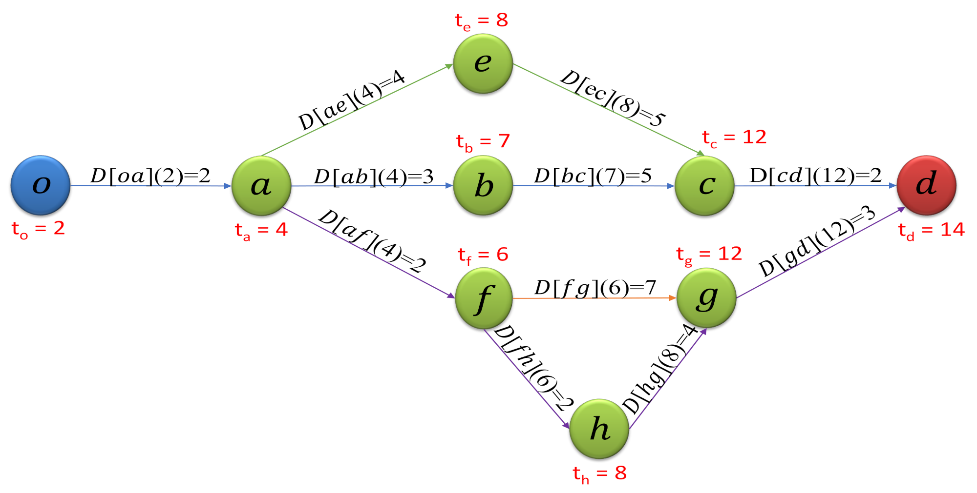
Figure 1 provides an example of a given subgraph H, whose quality indicators as an alternative graph are computed for a given departure time $t_o=2$ from o. In the example, the computations of the quality quantifications of H are based on the aforementioned functions and specifically for the totalDistance criterion they are grouped by a common denominator with respect to the contained four distinct shortest o-d paths: $\langle oa,ae,ec,cd\rangle$, $\langle oa,ab,bc,cd\rangle$, $\langle oa,af,fg,gd\rangle$, and $\langle oa,af,fh,hg,gd\rangle$. By considering the arcs of the first path, the travel time, the earliest arrival time, and the “share” contribution are determined as follows:

• Arc $oa$:
  $W\left[oa\right]\left(2\right)=D\left[oa\right]\left(Ar{r}_H[o,o]\left(2\right)\right)=D\left[oa\right]\left(2\right)=2$
  $Ar{r}_H[o,a]\left(2\right)=Ar{r}_H[o,o]\left(2\right)+D\left[oa\right]\left(Ar{r}_H[o,o]\left(2\right)\right)=2+2=4$
  $share\left[oa\right]\left(2\right)=\frac{W\left[oa\right]\left(2\right)}{D_H[o,o]\left(2\right)+W\left[oa\right]\left(2\right)+D_H[a,d]\left(Ar{r}_H[o,a]\left(2\right)\right)}=\frac{\left(2\right)}{\left(0\right)+\left(2\right)+(3+5+2)}=0.17$
• Arc $ae$:
  $W\left[ae\right]\left(2\right)=D\left[ae\right]\left(Ar{r}_H[o,a]\left(2\right)\right)=D\left[ae\right]\left(4\right)=4$
  $Ar{r}_H[o,e]\left(2\right)=Ar{r}_H[o,a]\left(2\right)+D\left[ae\right]\left(Ar{r}_H[o,a]\left(2\right)\right)=4+4=8$
  $share\left[ae\right]\left(2\right)=\frac{W\left[ae\right]\left(2\right)}{D_H[o,a]\left(2\right)+W\left[ae\right]\left(2\right)+D_H[e,d]\left(Ar{r}_H[o,e]\left(2\right)\right)}=\frac{\left(4\right)}{\left(2\right)+\left(4\right)+(5+2)}=0.31$
• Arc $ec$:
  $W\left[ec\right]\left(2\right)=D\left[ec\right]\left(Ar{r}_H[o,e]\left(2\right)\right)=D\left[ec\right]\left(8\right)=5$
  $Ar{r}_H[o,c]\left(2\right)=$ 2 + $min\{D_H\left[\langle oa,ae,ec\rangle \right]\left(2\right),D_H\left[\langle oa,ab,bc\rangle \right]\left(2\right)\}=$ 2 + $min\{11,10\}$ = 12
  $share\left[ec\right]\left(2\right)=\frac{W\left[ec\right]\left(2\right)}{D_H[o,e]\left(2\right)+W\left[ec\right]\left(2\right)+D_H[c,d]\left(Ar{r}_H[o,c]\left(2\right)\right)}=\frac{\left(5\right)}{(2+4)+\left(5\right)+\left(2\right)}=0.38$
• Arc $cd$:
  $W\left[cd\right]\left(2\right)=D\left[cd\right]\left(Ar{r}_H[o,c]\left(2\right)\right)=D\left[cd\right]\left(12\right)=5$
  $Ar{r}_H[o,d]\left(2\right)=Ar{r}_H[o,c]\left(2\right)+D\left[cd\right]\left(Ar{r}_H[o,c]\left(2\right)\right)=12+2=14$
  $share\left[cd\right]\left(2\right)=\frac{W\left[cd\right]\left(2\right)}{D_H[o,c]\left(2\right)+W\left[cd\right]\left(2\right)+D_H[d,d]\left(Ar{r}_H[o,d]\left(2\right)\right)}=\frac{\left(2\right)}{(2+3+5)+\left(2\right)+\left(0\right)}=0.17$

The overall quality of H in terms of the path non-overlappingness, stretch, and size-complexity are computed as follows:

$$\begin{array}{cc}\hfill \mathrm{totalDistance}\left(2\right)& =\left(share\right[oa\left]\right(2)+share[ab\left]\right(2)+share[bc\left]\right(2)+share[cd\left]\right(2\left)\right)\hfill \\ \hfill & +\left(share\right[af\left]\right(2)+share[fh\left]\right(2)+share[hg\left]\right(2)+share[gd\left]\right(2\left)\right)\hfill \\ \hfill & +\left(share\right[ae\left]\right(2)+share[ec\left]\right(2\left)\right)+\left(share\right[fg\left]\right(2\left)\right)\hfill \\ \hfill & =\frac{\left(2\right)}{\left(2\right)+3+5+2}+\frac{\left(3\right)}{2+\left(3\right)+5+2}+\frac{\left(5\right)}{2+3+\left(5\right)+2}+\frac{\left(2\right)}{2+3+5+\left(2\right)}\hfill \\ \hfill & +\frac{\left(2\right)}{2+\left(2\right)+2+4+3}+\frac{\left(2\right)}{2+2+\left(2\right)+4+3}+\frac{\left(4\right)}{2+2+2+\left(4\right)+3}+\frac{\left(3\right)}{2+2+2+4+\left(3\right)}\hfill \\ \hfill & +\frac{\left(4\right)}{2+\left(4\right)+5+2}+\frac{\left(5\right)}{2+4+\left(5\right)+2}+\frac{\left(7\right)}{2+2+\left(7\right)+3}\hfill \\ \hfill & =\frac{(2+3+5+2)}{(2+3+5+2)}+\frac{(2+2+4+3)}{2+(2+2+4+3)}+\frac{(4+5)}{2+(4+5)+2}+\frac{\left(7\right)}{4+\left(7\right)+3}\hfill \\ \hfill & =1+0.85+0.69+0.5=3.04\hfill \\ \hfill \mathrm{averageDistance}\left(2\right)& =\sum _{e\in E^{\prime }}\frac{W\left[e\right]\left(2\right)}{D_G[o,d]\left(2\right)·totalDistance\left(t_o\right)}=\sum _{e\in E^{\prime }}\frac{W\left[e\right]\left(2\right)}{12·3.04}\hfill \\ \hfill & =\frac{2+2+2+2+3+3+4+4+5+5+7}{12·3.04}=1.07\hfill \\ \hfill \mathrm{decisionEdges}& =|E^{\prime }|-(|V^{\prime }|-1)=11-8=3\hfill \end{array}$$

In order to assess the quality of an alternative graph, one should attempt to maximize the value of some target function, which is increasing in the $totalDistance$ and decreasing in the $averageDistance$, under the constraint that the $decisionEdges$ variable remains bounded. Unfortunately, achieving a lower value for $averageDistance$ may take away the ability of collecting high-degree disjoint (non-overlapping) paths, which would lead to a high value for $totalDistance$, since these criteria can be contradicting with each other. In this work, we choose to maximize a target function—the linear combination of the $totalDistance$ and $averageDistance$ variables. In particular, following [7,11], we aimed to maximize the value of the function

$$\begin{array}{cc}\hfill & targetFunction(H,o,d,t_o)=totalDistance+1-averageDistance\end{array}$$

(1)

under the constraint that the $DecisionEdges$ parameter is, at most, 10.

2.1. Computing Time-Dependent Shortest Paths

In this section, we review some fundamental techniques for computing a single time-dependent shortest $od$-path as a response to an arbitrary query $(o,d,t_o)$, which are used as subroutines throughout the paper.

2.1.1. Time-Dependent Dijkstra

The time-dependent variant of Dijkstra’s algorithm (TDD) [23] is a straightforward extension of the classical algorithm that computes the earliest-arrival-times “on the fly” when scanning (relaxing) the outgoing edges from a node. TDD grows a shortest-paths tree rooted at an origin o, for a given departure time $t_o$ from it. Analogously to the static case, TDD performs a breadth-first search (BFS) exploration of the graph, settling the nodes in increasing order of their tentative labels (representing the earliest-arrival-times from o, given the departure time $t_o$ from it), until the priority queue of labels becomes empty, or a given destination d is settled.

When settling a newly popped node u from the priority queue, all the outgoing edges are relaxed, implying new evaluations of the corresponding arc-traversal-time functions, given its label (i.e., the earliest-arrival-time at u) $t_u=Arr[o,u]\left(t_o\right)$ at that time. The resulting shortest-paths tree may vary for different departure time choices $t_o\in [0,T)$.

2.1.2. Reversed Time-Dependent Dijkstra

The reversed version of TDD (RTDD) grows a full shortest path tree rooted at a node d for a given arrival time $t_d$ at d. The differences from the original (forward) TDD are the following:

(a)

The arc relaxations are performed for the incoming arcs of the currently settled node.

(b)

The algorithm computes latest departure times from the arc tails “on the fly” during an arc-relaxation, by evaluating the inverse of the arc-arrival-time function (which is strictly increasing due to the strict FIFO property).

2.1.3. The CFLAT Oracle

The time-dependent oracle CFLAT [21] precomputes approximations $\overline{D}[\ell ,v]$ (called travel-time summaries) of minimum-travel-time functions $D[\ell ,v]$ from each element ℓ of a small set of carefully selected nodes (called landmarks), towards each reachable destination v. These travel-time summaries are succinctly represented as a collection of time-stamped minimum-travel-time trees. The appropriate construction of these summaries ensures both $(1+ϵ)$ approximation guarantees (for any given $ϵ>0$) for the landmark-to-destination travel-time functions $\overline{D}$ and efficient (subquadratic) space requirements.

2.2. Computing Alternative Graphs in Static Road Networks

In this section, we briefly review some typical approaches used for computing alternative graphs in time-independent (static) graphs.

2.2.1. Computing Alternative Routes within the Pareto Set

The Pareto algorithm [2,24,25] computes an alternative graph H by iteratively finding Pareto-optimal paths on a suitably defined objective cost vector. The idea is to use, as the first edge-cost vector, one of the single-criterion problems, while the second edge-cost is defined as follows: Initially, H only contains the shortest $od$-path. Then, all edges already belonging to H set their second cost function to their initial edge cost. All edges not belonging to H set their second cost function to zero.

A similar line of attack, for finding alternative routes via the multicriteria setting, is related to the so-called skyline-queries [3]. This approach was found to be feasible only for small graphs with a few thousands of nodes and three metrics for the arc costs, in which several-seconds query-response time is typically required.

The only multicriteria-based approach for alternative-routes, at least that we are aware of, that manages to efficiently compute alternative routes in million-node instances, is [26]. Based on the idea of personalized route planning, the paper discovers extreme solutions from the convex-pareto solution set that are sufficiently dissimilar with each other. In this direction, the idea is to use different weight vectors for the arc-cost metrics that provide significantly distinguishable routes for the commuter.

The deficit of this approach, nevertheless, is that it assumes that the route planner is aware of each commuter’s personalized secondary optimization criteria (which would render some of the alternative routes more attractive than others). Of course, this is not a typical situation, mostly because it is hard for a commuter to quantify secondary criteria, such as the scenic-ness or quietness of the routes. Moreover, this approach definitely excludes dominated paths (exactly due to their domination by some other path), even if it is not much worse than other paths but is also significantly distinct from other alternative routes. It also excludes pareto-optimal solutions that do not belong to the convex-pareto solution subset, irrespectively of their significance as alternative routes.

To recap, all these multicriteria-optimization based approaches for discovering alternative routes suffer from at least one of the following severe deficiencies:

(i)

They produce too many alternatives, causing severe computability issues even for moderate-size instances. Moreover, the produced solutions have only small deviations with each other, rendering them rather uninteresting, unless one really looks among them for actually distinguishable alternatives.

(ii)

Relaxing the domination criteria and fine-tuning the bounds to speed-up the computational requirements is non-trivial and time consuming.

(iii)

The secondary optimization criteria, which are rather personalized, are private information of the commuter, typically invisible to the route planner, and they are often difficult to quantify as concrete cost metrics, even for the commuters themselves.

2.2.2. Computing Alternative Routes from k-Shortest Path Solutions

The k-shortest path routing algorithm [4,5,6] finds the k-shortest paths in order of increasing cost. The disadvantage of this approach is that the computed alternative paths typically share too many edges, making it difficult for a human to actually distinguish them and make their own selection of a route. In order for really meaningful alternatives to be revealed, one should compute the k-shortest paths for very large values of k, at the expense of a rather prohibitive computational cost.

A more recent approach [27] was also based on the k-shortest path idea, essentially enumerating the shortest paths in increasing costs and then discarding paths that are already too similar with some of the previously selected paths. In this case as well, the proposed method appeared to be viable only for small-to-moderate network sizes.

2.2.3. The Plateau Method

The Plateau method [13] provides alternative $od$-paths by constructing “plateaus” that connect shortest subpaths. For a shortest-path tree $T_f$ from o and a reverse shortest-path tree $T_b$ from d, a $uv$-plateau is a $uv$-path that is a shortest subpath both in $T_f$ and $T_b$. The candidate paths via plateaus are constructed as follows: Dijkstra’s algorithm is used from o, and its reverse version from d, in order to produce, respectively, the trees $T_f$ and $T_b$. Consequently, for each $uv$-plateau in $T_f$ and $T_b$, the shortest $ou$-path in $T_f$ and the shortest $vd$-path in $T_b$ are connected at the endpoints of the $uv$-plateau, in order to form an alternative $od$-route. All these alternative $od$-routes are usually of high quality; however, there are too many for the commuter to digest, requiring a size decreasing filtration.

2.2.4. The Penalty Method

The Penalty method [14] provides alternative routes by iteratively running shortest-path queries and adjusting the weight of the arcs along the resulting path. Initially, a shortest-path query is performed. The resulting shortest path ${\pi }_{o,d}$ is chosen as the firest route, and it is then penalized by increasing the weight of all its constituent arcs.

Consequently, the method enters a loop in which, in each repetition, a new shortest-path query is executed in the graph with the modified weights. The resulting shortest path ${\pi }_{o,d}^{\prime }$ is again penalized, and, if it is substantially different from the previously selected $od$-routes and also not too long in the original graph, then it is appended to the solution set; otherwise, it is simply ignored. This repetitive process ends when a sufficient number of alternative routes, with the desired characteristics, are discovered, or the weight adjustments of $od$-paths bring no better results anymore. For a suitable penalty scheme, the resulting set of alternative $od$-routes can be of high quality.

3. The TDAG Algorithm

In this section, we present our new algorithm, TDAG, which, given a time-dependent road network $G=(V,E)$ with a small set $L\subset V$ of landmark-nodes accompanied with preprocessed landmark-to-node travel-time metadata and an arbitrary query $(o,d,t_o)$ of an origin-node $o\in V$, a destination-node $d\in V$, and a departure time $t_o\in [0,T)$ from o, computes a collection of meaningful (short and significantly non-overlapping) alternative $od$-routes. The solution set is succinctly represented by an alternative graph H, i.e., the subgraph of G induced by the arcs of the chosen $od$-routes. Of course, within H, there may exist even better combinations of $od$-routes for the query $(o,d,t_o)$, which are also considered as part of the solution.

TDAG is based on the rationale of the CFLAT oracle [21]. In a nutshell, it first grows two small-size TDD-balls, an origin-ball emanating from the origin and a destination-ball leading to the destination. It then connects the two balls by reconstructing (not necessarily the shortest, but short enough) paths ending in nodes of the destination-ball and starting from nodes within the origin-ball. This path construction is landmark-directed: the preprocessed information for the N landmarks of the origin-ball is exploited to direct these paths. A pruning step then takes over the responsibility of “cleaning” the resulting subgraph of uninteresting arcs. Eventually, the penalty method is applied to the final alternative graph, in order to conclude with a small set of meaningful alternative $od$-routes. TDAG also takes into account the following input parameters:

(i)

the number $N\in \mathcal{O}1$ of nearby landmarks that will be settled by TDD in the origin’s neighborhood;

(ii)

the upper bounds $maxAverageDistance$ for the $averageDistance$ criterion, $maxStretch$ for the maximum stretch of each $od$-path that is accepted as an alternative route of H, compared to the minimum-travel-time $D_H\left[od\right]\left(t_o\right)$ in the alternative graph H (Since TDAG essentially mimics the preprocessing of the CFLAT oracle [21], one can easily deduce that $D_H[o,d]\left(t_o\right)$ is a very good approximation of $D_G[o,d]\left(t_o\right)$, for all possible departure times from the origin.), and $maxDecisionEdges$ for the $decisionEdges$ criterion.

All these input parameters directly affect the size, the quality, and the computation time for constructing H.

TDAG consists of two building blocks, the preprocessing phase and the query algorithm, which will be presented in the rest of this section.

3.1. Preprocessing Phase of TDAG

Initially, TDAG selects a small subset $L\subseteq V\left(G\right)$ of landmark-nodes. There are various methods for the selection of L: either randomly, or according to some properties of the underlying graph, e.g., selection from boundary nodes of some balanced partition of the graph, or the selection of the most significant nodes in a node-ranking of the graph according to a centrality measure, such as betweenness-centrality [21].

In this work, we adopt one of the most successful methods for landmark selection, called Sparse-Random (SR), according to which, the landmarks are selected randomly and sequentially, so as to avoid having landmarks that are too close to each other. In particular, each new landmark ℓ is chosen uniformly at random from the subset of currently eligible non-landmark nodes. Right after the selection of the new element $\ell \in L$, a small neighborhood of non-landmark nodes around ℓ is excluded from all the subsequent landmark selections.

TDAG proceeds with the computation and succinct storage of timestamped shortest-path trees, from each landmark $\ell \in L$ towards all reachable destinations $v\in V$. The timestamp t of a given shortest-path tree $SP{T}_{\ell }\left(t\right)$ emanating from $\ell \in L$, denotes the assumed departure time from ℓ, for which $SP{T}_{\ell }\left(t\right)$ is indeed a shortest-path tree. For each landmark $\ell \in L$, the collection of SPTs

$$SP{T}_{\ell }:=\left\{SP{T}_{\ell }\left(t\right)|t\in T_{\ell }:=\left\{t_{\ell }^1,t_{\ell }^2,\dots ,t_{\ell }^{{\lambda }_{\ell }}\right\}\right\},$$

for carefully selected distinct (monotonically increasing) departure times, constitutes the travel-time summary stored for landmark ℓ during the preprocessing phase. The computation of SPTs from each landmarks is exactly the one conducted during the preprocessing phase of CFLAT [21]. Therefore, the preprocessing-time requirements can be fine-tuned so that they are subquadratic in the graph size. As for the required space (also subquadratic in the graph size [21]), in order to be able to efficiently handle continental-size time-dependent instances, we had to significantly improve the succinct representation of CFLAT’s travel-time summaries—in particular, how they are stored in the main memory.

The main intervention of this work, w.r.t. the preprocessing space requirements of CFLAT, is a lossless sparse matrix compression methodology for the succinct and space-efficient representation of all the timestamped SPTs from the landmarks, avoiding a considerable increase in the access time of the preprocessed information. In particular, the preprocessed data structure still conceptually contains, for each $\ell \in L$, the collection $SP{T}_{\ell }$ of timestamped shortest-path trees rooted at ℓ, which are optimal for the set of distinct, carefully selected departure times from ℓ, $T_{\ell }\subset [0,T)$. The selection of the set $T_{\ell }$ of distinct departure times from ℓ is such that, for all possible departure times $t\in [0,T)$, the collection $T_{\ell }$ contains at least one tree $SP{T}_{\ell }\left(i\right)$ providing, in worst case, a $(1+ϵ)$-approximation for $D_G[\ell ,v]\left(t\right)$:

$$\forall v\in V,D_{SP{T}_{\ell }\left(i\right)}[\ell ,v]\left(t\right)\le (1+ϵ)·D_G[\ell ,v]\left(t\right)$$

3.1.1. Data Structure for Timestamped Predecessors

The novelty of our succinct representation is the following: Rather than keeping a collection of trees per landmark, we maintain, for each pair $(\ell ,v)\in L\times V$, two sequences of the same length:

(i)

${\Delta }_{\ell ,v}$ is the sequence of sampled departure times from ℓ to v (in increasing order), and

(ii)

${\Pi }_{\ell ,v}$ is the sequence of predecessors of v in the corresponding $(\ell ,v)$-paths.

All the departure times for ${\Delta }_{\ell ,v}$ are assumed to be integers from $\{0,1,\dots ,86399\}$, considering an accuracy of seconds and a period of $T=$ 86,400 s. Rather than using 3 bytes per cell, we exploit the fact that most departure times are smaller than $2^{16}=$ 65,536 s. In particular, we keep an index $h_{\ell ,v}$ of the latest departure time in ${\Delta }_{\ell ,v}$, which is smaller than $2^{16}$. The first $h_{\ell ,v}$ cells in ${\Delta }_{\ell ,v}$ store the absolute departure time values, but the remaining cells only store the offset of the actual departure times from the value $2^{16}$. In this way, all the cells in ${\Delta }_{\ell ,v}$ require exactly 2 bytes. As for ${\Pi }_{\ell ,v}$, every cell is the relative position of the predecessor of v, in its in-neighborhood list. One byte per cell is sufficient for real-world instances whose maximum in-degree is a small constant.

A first observation of an initial implementation of this data structure was that a great deal of space was consumed for storing duplicates of exactly the same pairs of sequences for different landmark–destination pairs. For example, in the the continental-size EU instance with 18,010,173 nodes, for 16,000 landmarks, one would need to store 576,325,536,000 sequences. Nevertheless, we observed that there were only 1,632,168,375 distinct sequences (1,623,701,331 departure time sequences and 8,467,044 predecessor sequences). To avoid this waste of space, we chose to store only pairs of (4-byte) pointers to sequences, among all landmark–destination pairs.

After implementing this variant as well, we also observed that, in many cases, the same destination $v^{\ast }$ had many repetitions of the same pairs of (4-byte) pointers to sequences, over all the landmarks. Indeed, this is quite reasonable for landmarks located towards the same direction and roughly at the same distance from $v^{\ast }$. In order to avoid these repetitions of pairs of long pointers (8 bytes in total), we proceeded as follows (cf. Figure 2): We maintained a landmark-indexed dictionary $Ldic{t}_{v^{\ast }}$ per destination $v^{\ast }$, whose value for a key ${\ell }^{\ast }\in L$ is a pointer $s^{\ast }$ to the cell of an array $S_{v^{\ast }}$ containing a unique pair $(p^{\ast },d^{\ast })$ of pointers to the sequences ${\Delta }_{{\ell }^{\ast },v^{\ast }}$ and ${\Pi }_{{\ell }^{\ast },v^{\ast }}$.

The size $|S_{v^{\ast }}|$ is exactly the number of distinct pairs of pointers (to sequences) involving $v^{\ast }$, among all landmarks and, on average, is significantly smaller than $\left|L\right|$. Each cell of $S_{v^{\ast }}$ requires 8 bytes. On the other hand, for $Ldic{t}_{v^{\ast }}$, we used bit-level representation of the stored values, with each cell consuming only ${log}_2\left(\right|S_{v^{\ast }}|+indeg\left(v^{\ast }\right))$ bits. Even for 16,000 landmarks, this was, at most, 14 bits per cell.

Finally, we observed from real-world instances that, more often than not, a node $v^{\ast }$ might always have the same predecessor, independently of landmarks and departure times. In those cases, rather than storing $Ldic{t}_{v^{\ast }}$ and $S_{v^{\ast }}$, we simply stored this unique predecessor for $v^{\ast }$.

3.1.2. Lookup Procedure for Timestamped Predecessors

The lookup operation of preprocessed information, in order to obtain a time-dependent predecessor per landmark-to-vertex pair, is a procedure that is repeatedly used in the path-collection phase of the TDAG query algorithm (cf. PHASE-2 in Section 3.2). Briefly, the lookup operation takes, as input, a triple $(\ell ,v,t_{\ell })$ of a landmark $\ell \in L$, a current node $v\in V$ and a departure time $t_{\ell }\in [0,T)$ from ℓ. The lookup procedure starts by locating ${\Delta }_{\ell ,v}$, and then conducts a binary search in it, to locate the closest sampled departure times $de{p}_i\le t_{\ell }<de{p}_{i+1}$, in time $\mathcal{O}(log(\left|{\Delta }_{\ell ,v}\right|\left)\right($. For a constant number of sampled departure times from ℓ towards v, this is also the $\mathcal{O}$(1) time.

Then, the corresponding predecessors of v are located at positions i and $i+1$ of ${\Pi }_{\ell ,v}$, and, thus, are retrieved also in $\mathcal{O}$(1) time. Since the number of sampled departure times only partitions the period $[0,T)$ in small time intervals, it is independent of the network size (e.g., for the EU instance, the maximum length of a sampled departure times sequence is 4407). Therefore, the entire lookup procedure takes $\mathcal{O}$(1) time (e.g., at most 13 comparisons, even for EU).

Due to this novel methodology for the succinct representation of the preprocessed data, preprocessing a large number of landmarks is now possible, even for continental-size datasets. In terms of performance, this novel storage scheme provides a cache-friendly gain that beats the overhead of the bit-field and bit-mask extraction operations. This, in turn, leads to results of higher quality and significantly lowers the observed relative error of the travel-time approximations in the summaries of the landmarks.

3.2. Query Algorithm of TDAG

The TDAG query algorithm executes three sequential phases for serving a query $(o,d,t_o)\in V\times V\times [0,T)$.

PHASE 1: Landmark Settlement

A forward TDD tree $SP{T}_o\left(t_o\right)$ is grown from $(o,t_o)$ until either the destination-node d is settled or a set $F=SP{T}_o\left(t_o\right)L$ of the $\left|F\right|=N$ closest landmarks are settled (whichever comes first). Subsequently, a reverse BFS tree $RBF{S}_d$ from d is constructed that ignores, totally, the traversal-times of the arcs and exploring the neighborhood around d in a backward fashion. The growth of $RBF{S}_d$ is interrupted when its size becomes equal to $|RBF{S}_d|=c·|SP{T}_o\left(t_o\right)|$, for some constant $c\ge 1$. Our experimental analysis showed that $c=1.2$ is an appropriate choice.

We experimented also with growing a reverse TDD tree towards d; however, this approach was more time-consuming, and the resulting alternative graph, to be constructed in the next phases, was eventually similar to the one constructed using the reverse BFS tree from d.

PHASE 2: Path Collection

Using the preprocessed data, our next task was to construct a subgraph of the approximate shortest paths from the N landmarks $\ell \in F$, with their own departure times $t_{\ell }$, which were already computed in PHASE 1, towards each leaf node of $RBF{S}_d$. This was done as follows: For each leaf-node v of $RBF{S}_d$ and landmark $\ell \in F$ with departure time $t_{\ell }$, we recursively move backwards from v towards ℓ by recursively looking-up predecessors in the timestamped shortest-path trees $SP{T}_{\ell }\left(i\right)$ and $SP{T}_{\ell }(i+1)$ for which it holds that $t_{\ell }^i\le t_{\ell }<t_{\ell }^{i+1}$. All the arcs that participate in these $(\ell ,v)$-paths, for all landmarks $\ell \in F$ and all leaves v of $RBF{S}_d$, become marked.

The initial alternative graph H consists, then, of the union of the two trees $SP{T}_o\left(t_o\right)$ and $RBF{S}_d$ of PHASE 1, with the set of all the marked arcs during PHASE 2.

We continue by expanding the forward TDD tree $SP{T}_o\left(t_o\right)$ of PHASE 1 towards d, by working only in the subgraph H, until all the nodes in H are settled. This allows us to obtain a tentative arrival time ${\tilde{t}}_d$ at d:

$${\tilde{t}}_d=t_o+D_H[o,d]\left(t_o\right)\le t_o+\underset{\ell \in F}{min}\{D_G[o,\ell ]\left(t_o\right)+\overline{D}[\ell ,d](t_o+D_G[o,\ell ]\left(t_o\right))\}$$

where $\overline{D}[\ell ,d]\left(t\right)$ is the upper-bounding $(1+ϵ)$-approximate travel-time function from ℓ to v, stored in the preprocessed data of TDAG. As was proved in [21], ${\tilde{t}}_d$ is a constant upper-bound of the earliest-arrival-time $t_d=t_o+D_G[o,d]\left(t_o\right)$. The quality of this upper bound depends on the choice of the precision $ϵ$ of the preprocessed information, the number N of settled landmarks within $SP{T}_o\left(t_o\right)$, and the size of the reverse BFS tree $RBF{S}_d$.

PHASE 3: Pruning of the Alternative Graph

The graph H produced by PHASE 2 is already smaller than G. Nevertheless, it is further pruned so as to meet the three quality criteria for an alternative graph: small path overlapping, small stretch, and small size. This is done in three steps.

Step 3.1: 

Enforcement of the small stretch. We first aim at a loose pruning over H, in order to obtain a subgraph containing candidate $od$-paths with reasonable travel-times. Towards this direction, we consider the rationale of the via-node shortest $od$-routes. In particular, any node v in H whose shortest travel-time from o to d via v is greater than the targeted upper-bound, i.e., $D_H[o,v]\left(t_o\right)+D_H[v,d](t_o+D_H[o,v]\left(t_o\right))>maxStretch·D_H[o,d]\left(t_o\right)$, is removed.

Step 3.2: 

Decrease in the number of candidate$od$-routes. For further reducing the number of the candidate $od$-paths, we initially use the Plateau method [11,13] within H, by having previously run TDD from $(o,t_o)$ and RTDD from $(d,t_o+D_H[o,d]\left(t_o\right))$. Any arc not belonging to the resulting Plateau candidate $od$-paths is removed from H. The Penalty pruning method [11,14] is then applied to the resulting subgraph, in order to prune it even further. At each Penalty iteration, TDD runs on H, computing a new time-dependent shortest path ${\pi }_{o,d}$, whose constituent arcs are marked and are then appended to the solution set $E_s$. Additionally, all the arcs in $E_s$, and the all the arcs incident to nodes of ${\pi }_{o,d}$, are penalized with increasing the penalty factors $p\left(e\right)$ and $r\left(e\right)$, respectively, both initially set to 0.

In particular, for each arc $e=uv\in E_s$, its travel-time is increased to $D\left[e\right]{\left(t\right)}^{\left(penalized\right)}=(p{\left(e\right)}^{\left(current\right)}+1)D\left[e\right]{\left(t\right)}^{\left(original\right)}$; otherwise, if u or v are nodes in ${\pi }_{o,d}$ and e is not an arc of ${\pi }_{o,d}\cup E_s$, its travel-time is increased to $D\left[e\right]{\left(t\right)}^{\left(penalized\right)}=(r{\left(e\right)}^{\left(current\right)}+1)D\left[e\right]{\left(t\right)}^{\left(original\right)}$. The penalty factors of the affected arcs are increased at the end of each step to $p{\left(e\right)}^{\left(new\right)}=p{\left(e\right)}^{\left(old\right)}+p_c$ and $r{\left(e\right)}^{\left(new\right)}=r{\left(e\right)}^{\left(old\right)}+r_c$, where $p_c>0$ and $r_c>0$ are constants.

The process is repeated until a sufficient number of alternative paths are found or the travel time adjustments of ${\pi }_{o,d}$ paths bring no better results. Eventually, all the unmarked arcs are removed from H. In order to speedup the Penalty method at path computation, the time-dependent variant of $A^{\ast }$[28,29] can be used in place of TDD. For each node of H, its remaining distance towards d, which was already computed from RTDD during the Plateau substep, can be used as a lower bound for the time-dependent $A^{\ast }$ heuristic.

Step 3.3: 

Reduction in complexity of the alternative graph. The final pruning of H is performed via a ranking procedure. Initially, if a path ${\pi }_{x,y}$ in H has $outdeg\left(x\right)\ge 2$ and $indeg\left(y\right)\ge 2$, and $\forall v\in {\pi }_{x,y}-\{x,y\}$$outdeg\left(v\right)=indeg\left(v\right)=1$ (i.e., it increases by one the $decisionEdges$), then it is considered as a decision-path and it is ranked by the function $rank({\pi }_{x,y},t)={\sum }_{e\in {\pi }_{x,y}}$$\left(share\right[e\left]\right(t)-stretch[e\left]\right(t\left)\right)$ that represents the contribution of ${\pi }_{x,y}$ in terms of $averageDistance$ and $totalDistance$ in H.

The ranked decision paths are then sorted by increasing ranking order in a priority queue Q. Consequently, an iterative procedure starts where, in each iteration, a path ${\pi }_{x,y}$ is dequeued from Q. If the condition $outdeg\left(x\right)\ge 2$ and $indeg\left(y\right)\ge 2$ remains in effect, then ${\pi }_{x,y}$ is removed from H, leading to a decrease by one of the parameter $decisionEdges$. After the removal of ${\pi }_{x,y}$, if, for $v\in \{x,y\}$, it holds that $outdeg\left(v\right)=indeg\left(v\right)=1$, then a new decision path $\pi$ is revealed that has v as an internal node. $\pi$ is ranked and inserted in Q, in order to be considered along with the rest of decision paths. The iterative procedure stops when $decisionEdges\le maxDecsionEdges$.

3.3. Analysis of TDAG’s Preprocessing Phase and Query Algorithm

In this section, we provide a theoretical analysis for the quality of the alternative graph produced by TDAG, by means of the stretch of the optimal $od$-path in the alternative graph H, compared to the one in the original graph G.

Since TDAG employs a series of heuristic improvements, which make it difficult to provide a theoretical analysis, we focus here on a simplified variant of TDAG without any heuristic improvements, which we shall explain in detail later on.

Before that, we start with our working assumptions on the input instance. We consider a directed graph $G=(V,E)$ with $n=\left|V\right|$ vertices and $m=\left|E\right|$ arcs, which is sparse: $m\in \mathcal{O}n$. G is accompanied with a time-dependent cost metric, succinctly represented by periodic, continuous, pwl arc-traversal-time functions $D\left[uv\right]:[0,T)\mapsto {\mathbb{R}}_{>0}$. All time-dependent distances in this metric are indeed the minimum-travel-times $D[o,d]\left(t_o\right)$, for each pair of vertices $(o,d)\in V\times V$ and departure time $t_o\in [0,T)$ from the origin o.

Apart from the travel-times metric, we also consider the Dijkstra-Ranks metric for vertex-pairs: For any pair $(o,d)\in V\times V$ and departure time $t_o\in [0,T)$, the (also time-dependent) Dijkstra-Rank value, $DR[o,d]\left(t_o\right)$ is the cardinal number of d (i.e., its position in the settling order) when growing a forward TDD ball from $(o,t_o)$.

For theses two metrics that we consider, we make the following assumptions that have also been considered in previous works concerning time-dependent oracles, e.g., in [22].

Assumption 1

(Bounded Travel-Time Slopes). All the minimum-travel-time slopes are bounded in a given interval $[{-\Lambda }_{min},{\Lambda }_{max}]$, for the given constants ${\Lambda }_{min}\in [0,1)$ (${\Lambda }_{min}<1$ due to the FIFO property) and ${\Lambda }_{max}\ge 0$.

Assumption 2

(Bounded Opposite Trips). The ratio of minimum-travel-times in opposite directions between two vertices for any specific departure time, but not necessarily via the same path, is upper bounded by a given constant $\zeta \ge 1$.

Assumption 3

(Min-Travel-Times vs. Dijkstra-Ranks). There exist constants λ $,c_1,c_2\in \mathcal{O}1$ and functions $f\left(n\right)\le {log}^{c_1}\left(n\right),g\left(n\right)\le c_{2}log\left(n\right)$, s.t. the following hold:

(i) 

$DR[o,d]\left(t_o\right)\le f\left(n\right)·{\left(D[o,d]\left(t_o\right)\right)}^{\lambda }$, and

(ii) 

$D[o,d]\left(t_o\right)\le g\left(n\right)·{\left(DR[o,d]\left(t_o\right)\right)}^{1/\lambda }$.

Analogous inequalities hold for the static free-flow and the full-congestion metrics,$D^{\left(f\right)}$ and $D^{\left(c\right)}$.

Our next consideration is the preprocessed data-structure that is created by a time-dependent oracle (e.g., the CFLAT oracle in [22]). We start with an i.u.a.r. (i.e., independent and uniformly at random, without repetitions) selection of a small subset $L\subset V$ of landmark-vertices: each vertex $v\in V$ is chosen to be included in L with probability $\rho \in (0,1)$, independently of the other vertices. The preprocessed data structure succinctly represents the upper-bounding functions $\overline{D}[\ell ,v]:[0,T)\mapsto {\mathbb{R}}_{>0}$ of the (unknown) minimum-travel-time functions $D_G[\ell ,v]:[0,T)\mapsto {\mathbb{R}}_{>0}$, for all landmark-to-vertex pairs $(\ell ,v)\in L\times V$.

Our precondition is that these upper-bounding functions are also periodic, continuous, pwl, and constitute $(1+ϵ)$-approximations of the optimal travel-time functions. The variant of the TDAG query algorithm that we consider, called TDAGsimple, considers that $N=1$, i.e., it attempts to exploit only the closest landmark from the origin of the route. We explain the main steps of this query algorithm for alternative routes in Figure 3.

In order to proceed with the analysis of TDAGsimple, we first recall a theorem that concerns the analysis of the FCA${}^{+}$ query algorithm for computing an (approximation of an) earliest-arrival-time route in sparse, time-dependent networks:

Theorem 1

([15]). If a TD-instance, with $m\in \mathcal{O}\left(n\right)$ and compliant with Assumptions 1, 2 and 3 is preprocessed using ${\mathrm{BIS}}^{+}$ for constructing travel-time summaries from $\rho n$ i.u.a.r chosen landmarks, then the expected preprocessing space $S_{{\mathrm{BIS}}^{+}}$ and time $P_{{\mathrm{BIS}}^{+}}$ are

$$\begin{array}{ll}\mathbb{E}\left\{S_{{\mathrm{BIS}}^{+}}\right\}& \in \mathcal{O}(\rho n^2(K^{\ast }+1))\hfill \\ \mathbb{E}\left\{P_{{\mathrm{BIS}}^{+}}\right\}& \in \mathcal{O}(\rho n^2(K^{\ast }+1)[log\left(n\right)+loglog\left(K_{max}\right)])=\mathcal{O}(\rho n^2(K^{\ast }+1)log\left(n\right))\hfill \\ \mathbb{E}\left\{Q_{{\mathrm{FCA}}^{+}}\right\}& \in \mathcal{O}\left(1/\rho \right)\left[log\left(1/\rho \right)+loglog\left(K_{max}\right)\right]=\mathcal{O}\left(1/\rho \right)log\left(1/\rho \right)\end{array}$$

For the approximation guarantee,${\mathrm{FCA}}^{+}$returns either an exact$od$-path or approximate$od$-path via the nearest landmarkℓs.t.$D[o,d]\left(t_o\right)\le R_o+\overline{D}[{\ell }_o,d](t_o+R_o)\le (1+\epsilon )·D[o,d]\left(t_o\right)+\psi ·R_o\le (1+\epsilon +\psi )·D[o,d]\left(t_o\right),$where$R_o=D[o,\ell ]\left(t_o\right)$is the minimum-travel-time toℓ, and$\psi =1+{\Lambda }_{max}(1+\epsilon )(1+2\zeta +{\Lambda }_{max}\zeta )+(1+\epsilon )\zeta$is a constant that only depends on the parameters of the travel-times metric but is independent of the network size.

The following theorem provides a similar analysis for the query time and the approximation guarantee of TDAGsimple (the preprocessing requirements remain the same).

Theorem 2

TDAGsimple has the expected time-complexity$\mathcal{O}$), and also returns an alternative graph H in which the minimum-travel-time for $(o,d,t_o)$is, at most, a constant approximation of the minimum-travel-time for$(o,d,t_o)$within G:$D_H[o,d]\left(t_o\right)\le \alpha ·D_G[o,d]\left(t_o\right)$, for some constant$\alpha =1+ϵ+\psi \in \mathcal{O}\left(1\right)$.

Proof 

(sketch). The expected size of the landmark set is $\mathbb{E}\left\{\right|L\left|\right\}\in \mathcal{O}\left(\rho n\right)=\mathcal{O}\left(n^{1-\delta }\right)$. Moreover, by a simple application of Chernoff Bounds, we know that $\left|L\right|\in (1\pm 1)·n^{1-\delta }$, with high probability.

The expected size of the forward TDD-ball grown, cf. step 1, is $\mathbb{E}\left\{\right|SPT(o,t)\left|\right\}\in \mathcal{O}\left(\frac{1}{\rho }\right)=\mathcal{O}\left(n^{\delta }\right)$. Again, by a simple application of Chernoff Bounds, it can be shown that $\left|SPT(o,t)\right|\in (1\pm \mathrm{o}(1\left)\right)·n^{\delta }$, with high probability. The expected time-complexity to construct this ball is $\mathcal{O}\left(n^{\delta }\right)$.

The size of the reverse BFS ball grown in step 4 is chosen as $|RBF{S}_d|\in n^{\gamma }$. In the original version of the TDAG algorithm (which we implemented in this work), we considered the case where $|RBF{S}_d|\in \mathcal{O}(\left|SPT\right(o,t\left)\right|)$, i.e., $\gamma =\delta$. For our analysis here, we consider the more general case where the BFS ball is chosen independently of the forward TDD ball (e.g., we could select $\gamma =\frac{\delta }{3}$, in order to reduce the number of paths to reconstruct in step 7). The time-complexity for step 4 is linear in the size of the BFS ball, i.e., $\mathcal{O}\left(n^{\gamma }\right)$.

The expected size of the reverse TDD ball, cf. step 6, is $\mathbb{E}\left\{|TD{D}_r|\right\}\in \mathcal{O}\left(n^{\gamma }\right)$. This is because of the facts that G is a sparse graph, and moreover the Dijkstra-Rank and the minimum-travel-time metrics are correlated within polylogarithmic factors (a consequence of Assumption 3).

The expected time for constructing all the landmark-to-vertex paths in step 7 is $\mathcal{O}\left(n^{1+\gamma }\right)$, since there exist $\mathcal{O}\left(n^{\gamma }\right)$ leaves in the BFS ball, and each path consists of, at most, $n-1$ edges.

The overall running time of TDAGsimple is dominated by step 7 and is, therefore, $\mathcal{O}\left(n^{1+\gamma }\right)$.

As for the approximation guarantee, within the constructed alternative graph H, the earliest-arrival-time at d when departing from $(o,t_o)$ is $D_H[o,d]\left(t_o\right)\le {\overline{t}}_d$. To see this, consider the leaf-vertex v in $RBF{S}_d$, which also belongs to the approximating $\ell d$-path $\overline{\pi }[\ell ,d]$, that reaches d at time (at most) ${\overline{t}}_d$, when departing from $(\ell ,t_{\ell })$. The path $\overline{\pi }[\ell ,d]$ is not necessarily a subgraph of H. Nevertheless, its subpath $\overline{\pi }[\ell ,v]$ exists in H. Moreover, the optimal path $\widehat{\pi }[v,d]$ also exists in H. By following $\overline{\pi }[\ell ,v]$, we reach v at time (at most) ${\tilde{t}}_v$. It also holds that ${\widehat{t}}_v\ge {\tilde{t}}_v$, because ${\widehat{t}}_v$ is the latest-departure-time from v that reaches $(d,{\overline{t}}_d)$. Therefore, if from $(\ell ,t_{\ell })$ we follow the path $\overline{\pi }[\ell ,v]\oplus \widehat{\pi }[v,d]$, then we can be sure that the arrival time at d is, at most, ${\overline{t}}_d$, essentially due to the FIFO property in the travel-times metric:

$$\begin{array}{cc}\hfill {\overline{t}}_v& \ge {\widehat{t}}_v=t_{\ell }+\overline{D}[\ell ,v]\left(t_{\ell }\right)\hfill \\ \hfill {\overline{t}}_v+D\left[\widehat{\pi }[v,d]\right]\left({\overline{t}}_v\right)& \le {\widehat{t}}_v+D\left[\widehat{\pi }[v,d]\right]\left({\widehat{t}}_v\right)={\widehat{t}}_v+D[v,d]\left({\widehat{t}}_v\right)={\overline{t}}_d\hfill \end{array}$$

It is already known (cf. Theorem 1) that the approximate travel-time ${\overline{t}}_d-t_o$ is an $(1+ϵ+\psi )$-approximation of the minimum-travel-time in G, $D[o,d]\left(t_o\right)$, and thus this approximation guarantee also holds for $D_H[o,d]\left(t_o\right)$. □

4. Experimental Evaluation

In this section, we present our experimental study to assess the practical performance of the TDAG query algorithm for providing alternative routes in real-world time-dependent road networks.

4.1. Experimental Setup and Goal

TDAG was implemented in C++ (GNU GCC version 9.3.0). All the experiments were conducted on an AMD Ryzen Threadripper 3960X 24-Core 3.8 GHz Processor, with 256 GB of RAM, running Ubuntu Linux (20.04 LTS). We used 24 threads for the preprocessing phase of CFLAT [21], using $ϵ=0.1$ as the preprocessing precision.

Three typical benchmark instances for testing speedup techniques and oracles in time-dependent road networks were used in our experiments, kindly provided to us by TomTom and PTV for scientific purposes.

(BE)

The real-world instance of Berlin, provided by TomTom, has 473,253 nodes and 1,126,468 arcs. It is accompanied with arc-traversal-time functions taken from historical data of a working day (Tuesday) in a typical urban environment.

(GE)

The real-world instance of Germany, provided by PTV, has 4,692,091 nodes and 10,805,429 arcs. The arc-traversal-time functions represent a typical working day.

(EU)

The instance of Western Europe, provided by PTV, has 18,010,173 nodes and 42,188,664 arcs. It is a synthetic time-dependent benchmark instance that is typically considered in the related literature.

The TDAG query algorithm was executed on a single thread. For the sake of comparison, in all the query algorithms that were evaluated in this work, we used the same set of 10,000 queries chosen i.u.a.r. from $V\times V\times [0,T)$ in each instance, for randomly selected departure times from $[0,T)$. The static (forward-star) variant of the PGL library [30] was used for the graph representation. For Dijkstra-based algorithms, we used as priority queue Sander’s implementation (http://algo2.iti.kit.edu/sanders/programs/spq/, accessed on September 2020) of the sequence heap [31].

In [21], various methods were considered for the selection of the landmark set, significantly influencing the performance of CFCA (subroutine of TDAG). In our experimental evaluation of TDAG, we consider the sparse-random (SR) landmark-selection method that provides the best performance [21]: the landmark nodes are chosen sequentially, each new landmark is chosen i.u.a.r. from the remaining nodes, and excludes a free-flow neighborhood of nodes around it from future landmark selections. That selection is simple and yet effective on providing a high performance in TDAG.

The goal of our experimental evaluation was twofold:

(i)

To investigate the scalability of TDAG, i.e., how smoothly it trades higher query times with better quality guarantees for the resulting alternative graph H, using the value of N as our tuning parameter;

(ii)

To compare TDAG’s performance with the performances of straightforward time-dependent variants of existing techniques for constructing alternative graphs in static graphs [7,11], which serve as our baseline approaches.

In general, we assume that $D_H[o,d]\left(t\right)$ is equal or close enough to $D_G[o,d]\left(t\right)$, because of the TDD-based steps. Moreover, the relative error RelativeError, defined as

$$RelativeError=\frac{D_H[o,d]\left(t\right)-D_G[o,d]\left(t\right)}{D_G[o,d]\left(t\right)},$$

provides the observed approximation accuracy of H, that is, how close $D_H[o,d]\left(t\right)$ is to $D_G[o,d]\left(t\right)$, given that $D_H[o,d]\left(t\right)\ge D_G[o,d]\left(t\right)$.

4.2. Experimental Results

Our bit-level data compression technique (cf. Section 3.1) was found to be beneficial. The byte-based approach of CFLAT [21] for the succinct representation of the travel-time summaries of 2000 landmarks chosen with SR (SR2K) consumed space of $5.2$ GB in Berlin, $53.6$ GB in Germany, and $107.2$ GB in Europe. Using the new profiling, the bit-level based approach of TDAG, the preprocessed data for SR2K landmarks consumed space of $0.28$ GB in Berlin, $3.2$ GB in Germany, and $31.05$ GB in Europe. That is, the exploitation of the bit-level representation of a sparse matrix, without sacrificing the landmark and node indexing, leads to a significant reduction of about $70\%$ in space requirements, which, in turn, allows for the selection of larger landmark sets—especially for continental-size instances.

In

Table 1. Quality measures and execution times of TDAG. The background colors in certain cells highlight specific values of the target function and the corresponding execution times of TDAG’s query algorithm, per instance and landmark set. These values are used in Table 2, for comparison with the baseline approaches for time-dependent alternative routes.

Network	Landmark Set	N	Target Function	Total Dist.	Avg Dist.	Decision Edges	Relative Error (%)	Time (ms)	AG Size |V′|, |E′|
BE	SR4000	1	1.53	1.54	1.01	4.63	0.48	0.52	285, 288
		2	1.98	2.00	1.02	7.69	0.06	0.89	387, 393
		4	2.40	2.43	1.03	9.07	0.02	1.50	487, 495
		10	2.97	3.02	1.04	9.68	0.01	3.11	634, 642
		32	3.65	3.71	1.06	9.72	0.00	8.45	826, 835
		76	3.99	4.06	1.07	9.62	0.00	18.86	932, 946
		100	4.06	4.14	1.08	9.58	0.00	25.80	964, 973
		250	4.22	4.30	1.08	9.46	0.00	64.44	1057, 1065
GE	SR8000	1	1.50	1.51	1.01	8.60	0.51	1.31	536, 542
		2	1.93	1.94	1.02	9.96	0.06	2.80	737, 746
		8	2.77	2.81	1.04	9.93	0.00	11.38	1180, 1189
		18	3.26	3.32	1.06	9.86	0.00	28.89	1477, 1486
		25	3.45	3.51	1.07	9.80	0.00	43.33	1727, 1736
		64	3.88	3.96	1.09	9.63	0.00	135.04	2071, 2080
		100	4.02	4.11	1.09	9.54	0.00	213.05	2193, 2201
		200	4.15	4.25	1.10	9.40	0.00	384.15	2295, 2303
EU	SR16000	1	1.43	1.43	1.01	8.63	0.85	4.30	1397, 1405
		6	2.07	2.09	1.02	9.95	0.55	21.95	2124, 2133
		18	2.51	2.54	1.03	9.92	0.55	80.61	2722, 2731
		64	3.09	3.15	1.05	9.74	0.55	330.72	3763, 3772
		100	3.30	3.36	1.06	9.63	0.55	514.45	4384, 4393
		150	3.47	3.54	1.07	9.51	0.55	770.48	4553, 4562
		200	3.57	3.64	1.07	9.42	0.55	965.07	4837, 4846
		250	3.62	3.69	1.07	9.32	0.55	1237.80	4992, 5001

and

Table 2. Speedups of TDAG over DPP (with TDD) and APP (with $A^{\ast }$ and free-flow lower-bounds).

Network	Method	Target Function	Query Time	Speedup
BE	DPP	3.01	319.38	102.7
	TDAG vs. DPP	2.97	3.11
	APP	4.21	134.73	2.1
	TDAG vs. APP	4.22	64.44
GE	DPP	3.27	2623.36	90.8
	TDAG vs. DPP	3.26	28.89
	APP	4.17	1860.80	4.8
	TDAG vs. APP	4.15	384.15
EU	DPP	3.36	19,511.93	37.9
	TDAG vs. DPP	3.30	514.45
	APP	3.89	10,266.29	8.3
	TDAG vs. APP	3.62	1237.80

, we report the results of our experimental evaluations of TDAG on the approximation accuracy RelativeError (relative error in %) and the various quality indicators (To simplify the notation, we omit, in the rest of the paper, the departure time t notation.) (cf. Section 2): $targetFunction$ $\left(TargetFunction\right)$, $totalDistance$ $\left(TotDist\right)$, averageDistance $\left(AvgDist\right)$, and $decisionEdges$ $\left(DecEdges\right)$. Similar to [11], in order to evaluate the quality of the constructed alternative graph, the aggregate quality indicator $TargetFunction$ is used, which is defined as follows:

$$TargetFunction=totalDistance+1-averageDistance$$

In all our experiments, the resulting alternative graphs were evaluated using the following constraints: $maxStretch\le 1.2$, $averageDistance\le 1.1$, and $decisionEdges\le 10$. In the path pruning step, multiple choices on penalty constants were tested. The best results were achieved by selecting up to $p_c=0.3$ and $r_c=0.1$.

Table 1 demonstrates the effect of the parameter N on the execution time of TDAG, as well as on the quality of the constructed AG. As N grows, PHASE 1 becomes computationally more expensive; however, the relative error rapidly drops towards 0 for BE and GE. This is due to the fact that, as N increases, the expanded (forward) TDD tree becomes larger, the resulting $od$-paths increase in number, and we also obtain more candidate $od$-paths providing an AG of better quality.

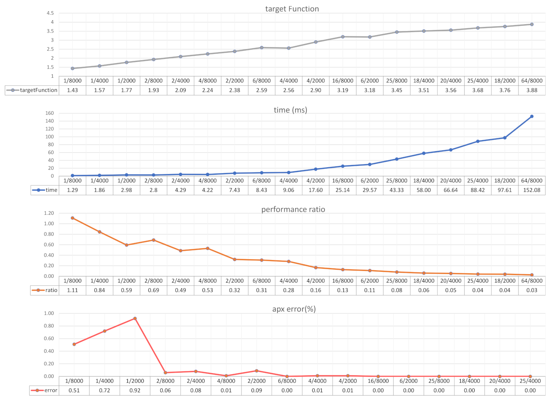
Figure 4 shows the quality (targetFunction) and run time performance of TDAG with respect to the number $\left|L\right|$ of landmarks and the selection of N for GE. Each increase of the targetFunction depends on collecting and processing a larger number of candidate alternative paths between origin o and destination d, which, in turn, requires a higher computation time. However, by increasing either $\left|L\right|$ or N, the error is reduced. The targetFunction obtains higher values either by a long TDD tree step or by a long predecessor tree step. The first case happens when $\left|L\right|$ is smaller—where landmarks are more distant from each other. The second case happens when $\left|L\right|$ is larger—where landmarks are less distant from each other.

As for EU, the relative error seems to stop at $0.55$ due to the steepest slopes of the earliest-arrival-time functions (which necessitate an increased number of sampled departure times during the preprocessing phase), the propagation of floating point rounding errors along the arcs of long paths, and the smaller density $\left|L\right|/\left|V\right|$ of the preprocessed landmarks, compared to the instances of BE and GE. All these issues can be tackled by affording more memory for the computations.

In Table 2, we present the results of the baseline approaches and their comparison to TDAG. DPP is a combination of the Plateau and the Penalty methods [7], which collects and evaluates the candidate $od$-paths using a greedy selection approach. In our time-dependent context, Dijkstra’s algorithm was replaced by its time-dependent variant, TDD. APP is, again, a combination of the Plateau and Penalty methods of [7,11], which uses the ALT pruner and filtering approach [11]. Dijkstra’s algorithm was, again, replaced by TDD, and for the lower bounds required by ALT the constant free-flow minimum-travel-time distances were used (i.e., each arc has a scalar cost corresponding to its minimum traversal-time).

DPP does not require prepossessing, while APP requires a linear-in-space and super-linear-in-time prepossessing phase for computing the lower bounds required by ALT. Regarding the computation of the alternative graph (column q-time in Table 2), both baseline approaches had a slow path collection phase. DPP constructs a subgraph H that is huge in size, using an expensive phase of pure TDD as there are no heuristics. APP improves the time of the path collection phase; however, the lower bounds are not tight for a time-dependent metric. In both cases, the achieved quality is high, at the cost of large processing times.

From Table 1 and Table 2, it is clear that, for all instances, the configurations of TDAG that achieve analogous aggregate quality required execution times that were about two orders of magnitude smaller than those of DPP. In particular, the achieved speedups were more than $102.7$ for BE, $90.8$ for GE, and $37.9$ for EU. Similarly, the configurations of TDAG achieving similar values of the target function were faster than APP by about one order of magnitude, as the instance size increased. In particular, the speedups were $2.1$ for BE, $4.8$ for GE, and $8.3$ for EU.

5. Conclusions

In this work, we presented TDAG, a novel algorithm for computing alternative routes in FIFO-abiding time-dependent road networks based on succinctly stored preprocessed travel information. One of TDAG’s strong features is that it can smoothly trade-off the quality of the resulting alternative graph with the required execution time via proper choices of its parameter N. This feature provides a significant advantage over all existing approaches, which have only one solution set of $od$-paths.

Our experimental evaluation, on two real-world instances and one synthetic instance, demonstrated that TDAG clearly outperformed both baseline approaches (DPP and APP), since it provided time-dependent alternative routes of the same quality as DPP and APP within smaller execution times. TDAG can also provide “quick-and-dirty” alternative routes with a speedup of more than 100 over both DPP and APP; however, it can continue its execution until it finds alternative routes of the same quality as DPP and APP and is still much faster (less than half time for BE and one fifth of time for GE) than these two baseline approaches.

Many different approaches and experiments have been left for future research, due to a lack of time, as the experiments with continental-sized road networks are very time consuming. Our plans for future work also concern a deeper analysis of the particular procedures that we use as well as some novel approaches and methods for the path collection phase and the pruning schemes. There is still plenty of space for improving the path aggregation phase and the penalty and ranking pruning steps to acquire the best qualitative alternative paths faster and with a reduced computational cost. In addition, further heuristics (e.g., exploiting the special features of road networks) should also be considered, in order to improve the overall performance of an algorithm to discover meaningful alternative routes.

References

- Bast, H.; Delling, D.; Goldberg, A.V.; Müller-Hannemann, M.; Pajor, T.; Sanders, P.; Wagner, D.; Werneck, R.F. Route planning in transportation networks. In Algorithm Engineering: Selected Results and Surveys; Kliemann, L., Sanders, P., Eds.; Springer: Berlin/Heidelberg, Germany, 2016; pp. 19–80. [Google Scholar]
- Delling, D.; Wagner, D. Pareto paths with SHARC. In International Symposium on Experimental Algorithms; Springer: Berlin/Heidelberg, Germany, 2009; pp. 125–136. [Google Scholar]
- Kriegel, H.P.; Renz, M.; Schubert, M. Route skyline queries: A multi-preference path planning approach. In Proceedings of the 26th International Conference on Data Engineering (ICDE), Long Beach, CA, USA, 1–6 March 2010; pp. 261–272. [Google Scholar]
- Eppstein, D. Finding the k shortest paths. J. Comput. 1998, 28, 652–673. [Google Scholar] [CrossRef] [Green Version]
- Feng, G. Finding k-shortest simple paths in directed graphs: A node classification algorithm. Networks 2014, 64, 6–17. [Google Scholar] [CrossRef]
- Yen, J.Y. Finding the k shortest loopless paths in a network. Manag. Sci. 1971, 17, 712–716. [Google Scholar] [CrossRef]
- Bader, R.; Dees, J.; Geisberger, R.; Sanders, P. Alternative route graphs in road networks. In International Conference on Theory and Practice of Algorithms in (Computer) Systems; Springer: Berlin/Heidelberg, Germany, 2011; pp. 21–32. [Google Scholar]
- Ittai, A.; Delling, D.; Goldberg, A.V.; Werneck, R.F. Alternative routes in road networks. In International Symposium on Experimental Algorithms; Springer: Berlin/Heidelberg, Germany, 2010; pp. 23–34. [Google Scholar]
- Kobitzsch, M. An alternative approach to alternative routes: Hidar. In European Symposium on Algorithms; Springer: Berlin/Heidelberg, Germany, 2013; pp. 613–624. [Google Scholar]
- Luxen, D.; Schieferdecker, D. Candidate sets for alternative routes in road networks. In International Symposium on Experimental Algorithms; Springer: Berlin/Heidelberg, Germany, 2012; pp. 260–270. [Google Scholar]
- Paraskevopoulos, A.; Zaroliagis, C. Improved Alternative Route Planning. In 13th Workshop on Algorithmic Approaches for Transportation Modelling, Optimization, and Systems (ATMOS); OpenAccess Series in Informatics (OASIcs); OASICS Dagstuhl Publishing: Saarbrücken, Germany, 2013; Volume 33, pp. 108–122. [Google Scholar]
- eCOMPASS Project, 2011–2014. Available online: http://www.ecompass-project.eu (accessed on 1 September 2020).
- Camvit: Choice Routing. 2009. Available online: http://www.camvit.com (accessed on 1 September 2020).
- Chen, Y.; Bell, M.G.H.; Bogenberger, K. Reliable pretrip multipath planning and dynamic adaptation for a centralized road navigation system. Trans. Intell. Transp. Syst. 2007, 8, 14–20. [Google Scholar] [CrossRef]
- Kontogiannis, S.; Zaroliagis, C. Distance oracles for time-dependent networks. Algorithmica 2016, 74, 1404–1434. [Google Scholar] [CrossRef]
- Dean, B.C. Shortest Paths in FIFO Time-Dependent Networks: Theory and Algorithms. Available online: https://people.cs.clemson.edu/~bcdean/tdsp.pdf (accessed on 20 July 2021).
- Dehne, F.; Masoud, O.T.; Sack, J.R. Shortest paths in time-dependent FIFO networks. Algorithmica 2012, 62, 416–435. [Google Scholar] [CrossRef]
- Foschini, L.; Hershberger, J.; Suri, S. On the complexity of time-dependent shortest paths. Algorithmica 2014, 68, 1075–1097. [Google Scholar] [CrossRef]
- Orda, A.; Rom, R. Shortest-path and minimum delay algorithms in networks with time-dependent edge-length. J. ACM 1990, 37, 607–625. [Google Scholar] [CrossRef] [Green Version]
- Batz, G.V.; Geisberger, R.; Sanders, P.; Vetter, C. Minimum time-dependent travel times with contraction hierarchies. J. Exp. Algorithmics (JEA) 2013, 18, 1.1–1.43. [Google Scholar] [CrossRef]
- Kontogiannis, S.; Papastavrou, G.; Paraskevopoulos, A.; Wagner, D.; Zaroliagis, C. Improved oracles for time-dependent road networks. arXiv 2017, arXiv:1704.08445. [Google Scholar]
- Kontogiannis, S.; Wagner, D.; Zaroliagis, C. Hierarchical time-dependent oracles. Algorithms Comput. (ISAAC) 2016, 64, 1–13. [Google Scholar]
- Dreyfus, S.E. An appraisal of some shortest-path algorithms. Oper. Res. 1969, 17, 395–412. [Google Scholar] [CrossRef]
- Hansen, P. Bicriterion path problems. In Multiple Criteria Decision Making Theory and Application; Springer: Berlin/Heidelberg, Germany, 1980; pp. 109–127. [Google Scholar]
- Queiros Vieira Martins, E. On a multicriteria shortest path problem. Eur. J. Oper. Res. 1984, 16, 236–245. [Google Scholar] [CrossRef]
- Barth, F.; Funke, S.; Storandt, S. Alternative Multicriteria Routes. In Algorithm Engineering & Experiments (ALENEX); SIAM: Philadelphia, PA, USA, 2019; pp. 66–80. [Google Scholar]
- Chondrogiannis, T.; Bouros, P.; Gamper, J.; Leser, U.; Blumenthal, D.B. Finding k-shortest paths with limited overlap. VLDB J. 2020, 29, 1023–1047. [Google Scholar] [CrossRef] [Green Version]
- Doran, J. An approach to automatic problem-solving. In First International Machine Learning Workshop (Machine Intelligence 1); Oliver and Boy: Edinburgh, UK, 1967; pp. 105–124. [Google Scholar]
- Hart, P.E.; Nilsson, N.J.; Raphael, B. A formal basis for the heuristic determination of minimum cost paths. Trans. Syst. Sci. Cybern. 1968, 4, 100–107. [Google Scholar] [CrossRef]
- Mali, G.; Michail, P.; Paraskevopoulos, A.; Zaroliagis, C. A new dynamic graph structure for large-scale transportation networks. In International Conference on Algorithms and Complexity—CIAC 2013; Springer: Berlin/Heidelberg, Germany, 2013; pp. 312–323. [Google Scholar]
- Sanders, P. Fast priority queues for cached memory. J. Exp. Algorithmics (JEA) 2000, 5, 7. [Google Scholar] [CrossRef]
Figure 1.
Evaluation of the quality-assessment criteria for a given alternative graph. For each node x, is the earliest arrival time at x, for departure time . We assume that . The minimum travel time is via .
Figure 2.
Data structure for the succinct representation of preprocessed information of TDAG.
Figure 3.
The pseudocode for TDAGsimple.
Figure 4.
The targetFunction, execution time, and ratio of targetFunction/time of TDAG at GE. In the first row of the horizontal axis, the tested combinations of are shown.