
Synthetic Experiences for Accelerating DQN Performance in Discrete Non-Deterministic Environments †


1
Organic Computing Group, University of Augsburg, 86159 Augsburg, Germany
2
Artificial Intelligence in Agricultural Engineering, University of Hohenheim, 70599 Stuttgart, Germany
*
Author to whom correspondence should be addressed.
†
This paper is an extended version of our paper published in 12th International Conference on Neural Computation Theory and Applications, Budapest, Hungary, 2–4 November 2020.
Algorithms 2021, 14(8), 226; https://0-doi-org.brum.beds.ac.uk/10.3390/a14080226
Submission received: 30 June 2021
/
Revised: 24 July 2021
/
Accepted: 26 July 2021
/
Published: 27 July 2021
(This article belongs to the Special Issue Algorithmic Aspects of Neural Networks)
Abstract
:State-of-the-art Deep Reinforcement Learning Algorithms such as DQN and DDPG use the concept of a replay buffer called Experience Replay. The default usage contains only the experiences that have been gathered over the runtime. We propose a method called Interpolated Experience Replay that uses stored (real) transitions to create synthetic ones to assist the learner. In this first approach to this field, we limit ourselves to discrete and non-deterministic environments and use a simple equally weighted average of the reward in combination with observed follow-up states. We could demonstrate a significantly improved overall mean average in comparison to a DQN network with vanilla Experience Replay on the discrete and non-deterministic FrozenLake8x8-v0 environment.
1. Introduction
In the domain of Deep Reinforcement Learning (RL), the concept known as Experience Replay (ER) has long since developed to become a well-known standard for many algorithms [1,2,3]. Initially designed as an extension for Q- and AHC-Learning [4], it has become an integral part of the Deep Q-Network (DQN) family. Here, it is mandatory to overcome instabilities in the learning phase [5]. Another positive effect that comes along with the use of ERs is an increased sample efficiency, which is achieved by reusing remembered transitions several times.
Being a key component for many Deep RL algorithms makes the concept of ER attractive for improvements and extensions. Most of them store real, actually experienced, transitions. Mnih et al. [2], for example, used the basic ER version to assist their DQN, and Schaul et al. [1] extended it to a version called Prioritized Experience Replay, which, instead of uniformly drawing, prefers experiences that promise greater learning successes. However, there are other approaches as well, and these extensions focus on the usage and creation of experiences that are synthetic in some way. An example of this is the so-called Hindsight Experience Replay [3] that saves trajectories of states and actions together with a corresponding goal. By replacing the goal with the last encountered state, a synthetic trajectory is created and saved together with the real one. The authors could show that this method promises great success in multi-objective problem spaces.
The contribution of our work is an ER-extension that uses synthetic experiences. A (not complete) list of (Deep) RL algorithms that use an ER is the following: DQN, DDPG or classic Q-Learning [6]. Our ER version is targeted to improve the performance of these algorithms in nondeterministic and discrete environments. To achieve this, we consider all the stored real state-transitions as the gathered knowledge of the underlying problem. Utilizing this knowledge, we are able to create synthetic experiences that contain an average reward of all related surroundings. This approach makes it possible to increase the sample efficiency even more because experiences are now also used for the generation of new and possibly better synthetic experiences. We use observed follow-up states to complete our so-called interpolated experiences and can support our learner in the exploration phase this way.
The evaluation is performed on the FrozenLake environment from the OpenAI Gym [7]. Offering a discrete state space in the form of a grid world, in combination with a non-deterministic state-transition-function, makes it a good choice to evaluate our algorithm on. To increase scientific relevance and validity, we evaluate three different state encodings and corresponding various deep network architectures.
The investigated problem is discrete and non-deterministic, and the averaging is a rather simple method as well, but the intention is to gain the first insights in this highly interesting field. We can reveal promising potential utilizing this very simple technique, and this work serves as a basis to build up further research on.
The present work is an extended version of [8]. In addition to the original publication, we used actual deep neural networks instead of a linear regression. We also investigated different state encodings, making the problem more difficult and interesting and also increasing the scientific validity. We tied up on the results of this paper and were able to define new questions to investigate. The key idea remains the same but is extended with deeper evaluation.
The paper is structured as follows: We start with a brief introduction of the ER and Deep Q-Learning in Section 2 and proceed with relevant related work in Section 3. In Section 4, we introduce our algorithm alongside with a problem description and the Interpolation Component that was used as an underlying architecture. The evaluation and corresponding discussion, as well as interpretation of the results, are presented in Section 5. The article closes with a conclusion and gives an outlook on future work in Section 6.
2. Background
In this section, we start with introducing the idea of the Experience Replay and continue with the presentation of Deep Reinforcement Learning basics as well as an explanation of why the former concept is mandatory here.
2.1. Experience Replay
The ER is a biologically inspired mechanism [4,9,10,11] to store experiences and reuse them for training later on.
An experience is defined as: , where denotes the start state, the performed action, the corresponding received reward and the follow-up state. To perform Experience Replay, at each time step t, the agent stores its recent experience in a data set . In an non-episodic/infinite environment (and also in an episodic one after enough time has gone by), we would run into the problem of limited storage. To counteract this issue, the vanilla ER is realized via a FiFo buffer, and old experiences are thrown away after reaching the maximum length.
This procedure is repeated over many episodes, where the end of an episode is defined by a terminal state. The stored transitions can then be utilized for training either online or in a specific training phase. It is very easy to implement ER in its basic form, and the cost of using it is mainly determined by the storage space needed.
2.2. Deep Q-Learning
The DQN algorithm is the combination of the classic Q-Learning [12,13] with neural networks and was introduced in [2,14]. The authors showed that their algorithm is able to play Atari 2600 games on a professional human level utilizing the same architecture, algorithm and hyperparameters for every single game. As DQN is a derivative of classical Q-Learning, it approximates the optimal action-value function:
However, DQN employs a neural network instead of a table to parameterize the Q-function. Equation (1) displays the maximum sum of rewards discounted by at each time-step t, which is achievable by a behaviour policy , after making an observation s and taking an action a. DQN performs a Q-Learning update at every time step that uses the temporal-difference error defined as follows:
Tsitsiklis et al. [5] showed that a nonlinear function approximator used in combination with temporal-difference learning, such as Q-Learning, can lead to unstable learning or even divergence of the Q-Function.
As a neural network is a nonlinear function approximator, several problems arise:
- the correlations present in the sequence of observations;
- the fact that small updates to Q may significantly change the policy and, therefore, impact the data distribution; and
- the correlations between the action-values and the target valuespresent in the td-error shown in Equation (2).
The last point is crucial because an update to Q will change the values of both the action-values and the target values. This change could lead to oscillations or even divergence of the policy. To counteract these issues, two concrete actions have been proposed:
- The use of an ER solves, as stated above, the two first points. Training is performed each step on minibatches of experiences , which are drawn uniformly at random from the ER.
- To remove the correlations between the action-values and the target values, a second neural network is introduced that is basically a copy of the network used to predict the action-values. The target-network is either frozen for a certain interval C before it is updated again or “soft” updated by slowly tracking the learned networks weights utilizing a factor . This network is responsible for the computation of the target action-values. [2,15]
We use the target network performing “soft” updates as presented above and extend the classic ER with a component to create synthetic experiences.
3. Related Work
The classical ER, introduced in Section 2.1, has been improved in many further publications. One prominent improvement is the so called Prioritized Experience Replay [1], which replaces the uniform sampling with a weighted sampling in favour of experience samples that might influence the learning process most. This modification of the distribution in the replay induces bias, and to account for this, importance-sampling has to be used. The authors show that a prioritized sampling leads to great success. This extension of the ER also changes the default distribution but uses real transitions and therefore has a different focus.
The authors of [16,17] investigated the composition of experience samples in the ER. They discovered that for some tasks, transitions made in an early phase when exploration is high are important to prevent overfitting. Therefore, they split the ER into two parts: one with samples from the beginning and one with actual samples. They also show that the composition of the data in an ER is vital for the stability of the learning process, and at all times, diverse samples should be included. Following these results, we try to achieve a broad distribution over the state space utilizing synthetic experiences (for most of our configurations).
Jiang et al. [18] investigated ERs combined with model-based RL and implemented a tree structure to represent a model of the environment. In their research, they learned a model of the problem and invented a tree structure to represent it. Using this model, they could simulate virtual experiences that they used in the planning phase to support learning. To increase sample efficiency, experience samples are stored in an ER. This approach has some similarities to the interpolation-based approach presented in this work but addresses other aspects, such as learning a model of the problem first.
Gu et al. [19] presented an interpolation of on-policy and off-policy model-free Deep Reinforcement Learning techniques. In this publication, an approach of interpolation between on- and off-policy gradient mixes likelihood ratio gradient with Q-Learning, which provides unbiased but high-variance gradient estimations. This approach does not use an ER and therefore differs from our work.
This work draws on the methods proposed in [20,21,22,23,24]. The authors used interpolation in combination with an XCS classifier System to speed up learning in single-step problems by using previous experiences as sampling points for interpolation. Our approach focuses on a DQN as a learning component and, more importantly, multi-step problems and therefore differs from this work. Anyhow, we adopted the so-called Interpolation Component that is introduced in more detail in Section 4.3.
4. Interpolated Experience Replay
In this Section, we present the FrozenLake problem and introduce our algorithm to solve it. We also introduce the Interpolation Component that serves as architectural concept.
4.1. Problem Description
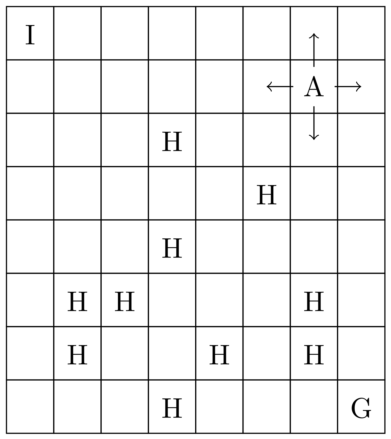
“FrozenLake” is one example of a non-deterministic world in which an action realised in a state may not consistently lead to the same follow-up state . FrozenLake is basically a grid world consisting of an initial state I, a final state G and frozen, as well as unfrozen tiles. The unfrozen tiles equal holes H in the lake and if the agent falls into one of such, he has to start from the initial state again. If the agent reaches G, he receives a reward of 1. The set of possible actions A consists of the four cardinal directions . Executing a concrete action (e.g., N) only results with a probability of in the corresponding field, but it is also possible that the agent instead performs one of the orthogonal actions (in our example: W or E) with the same probability of for each case. This behaviour makes the environment non-deterministic. Because there is a discrete number of states the agent can reach, we can denote the problem as discrete as well. The environment used for evaluation is the “FrozenLake8x8-v0” environment from OpenAI Gym [7], as depicted in Figure 1.
In addition to the described version, we changed the reward function to return a reward of in the case of falling into a hole and 5 for reaching the goal. As the first adaption is crucial for our approach, the second change helps the learner to solve the environment. Both changes intensify the received rewards and therefore the experienced transitions. Assigning a negative reward to the end of an episode (hole) makes it possible to calculate an average reward containing an additional value (see below). By testing different final rewards (goal), we could observe that the agent performed best with a reward of 5.
The decision to focus on the presented environment was taken because: (1) it is a relatively well-known problem in the RL community (OpenAI Gym); (2) our presented approach is designed for discrete and non-deterministic environments. To add more variability, we used three different state encodings (see Section 5.1).
The non-deterministic character of the problem comes with difficulties that are described in the following paragraph: If an action is chosen that leads the agent in the direction of the goal, but because of the slippery factor, it is falling into a hole, it additionally receives a negative reward and creates the following experience: . If this experience is used for a Q update, it misleadingly shifts the state-action value away from a positive value. We denote the slippery factor for executing a neighbouring action as , the resulting rewards for executing the two neighbouring actions as and and the reward for executing the intended action as and can then define the true expected reward for executing in as follows:
Following Equation (3), we define the experience that takes the state-transition function into account and that does not confuse the learner as the expected experience :
The learner will converge its state-action value after seeing enough experiences to:
A Q update with received (misleading) experiences comes with the effect of oscillation as the non-deterministic property of the environment creates rewards and follow-up states that might lead in completely opposite directions (e.g., brings the agent closer to the goal vs. ends the episode in a hole). In the original environment (reward for falling into a hole equals 0), this effect would also appear because the different follow-up states hold the same information. If the learner only receives experiences in the form of , the amount of time required to converge to could be decreased.
4.2. Averaging Rewards
The intention of our solution is to reduce the amount of training by the creation of synthetic experiences that are as similar as possible to . As a current limitation, we focus on estimating and use real observed follow-up states . That approach is possible because the environment is discrete (this represents a mandatory precondition of our algorithm). Discrete environments provide a limited amount of states and more important corresponding follow-up states, and it is possible to observe and remember them. In continuous environments, we would also need to predict the follow-up state next to the reward, and for this first investigation of the concept of interpolated experiences, we decided to keep it simple. To compute an accurate estimation of , we need to estimate first.
The set of all rewards that belong to the experiences that start in the same state and execute the same action can be defined as:
We use the rewards in to calculate the average and denote it as . This value holds as a good estimation of .
following this, we can then define as our estimation of as:
with
The accuracy of this interpolation correlates with the amount of transitions stored in the ER, which start in and execute . This comes from the fact that the effect of outliers can be mitigated from enough normal distributed samples. To achieve this, we defined an algorithm that triggers an interpolation after every step the agent takes. A query point is drawn via a sampling method from the state space, and all matching experiences:
where their starting point is equal to the query point , are collected from the ER. Then for every action , all experiences that satisfy are selected from in:
The resulting transitions are used to compute an average reward value . Utilizing this estimation, a synthetic experience for every distinct next state:
is created. This results in a minimum of 0 and a maximum of 3 synthetic experiences per action and sums up to a maximum of 12 synthetic transitions per interpolation depending on the amount of stored transitions in the ER. As with the amount of stored real transitions, which can be seen as the combined knowledge of the model, the quality of the interpolated experiences may get better. A parameter is introduced that determines the minimum amount of stored experiences before the first interpolation is executed. The associated pseudocode is depicted in Algorithm 1.
4.3. Interpolation Component
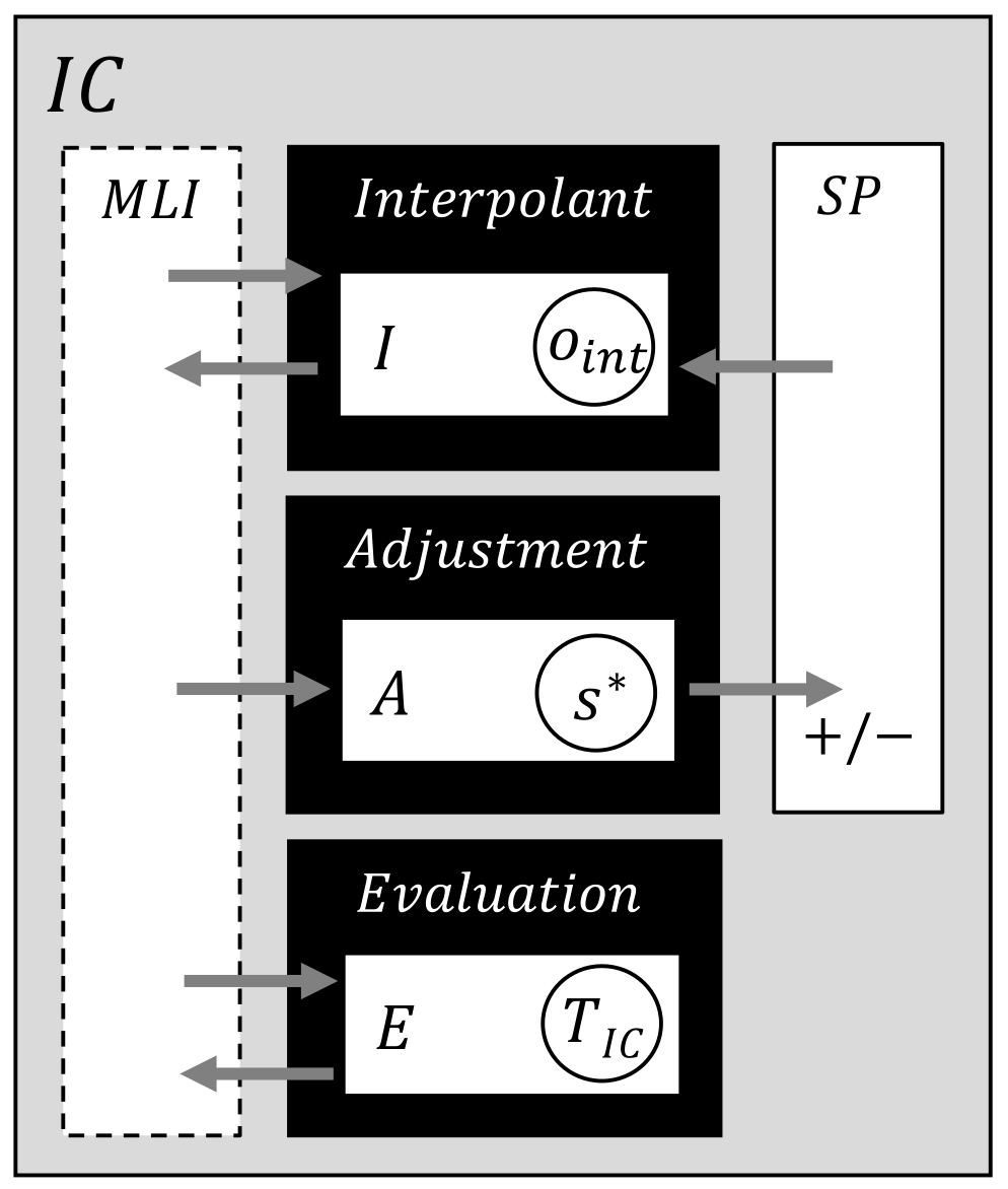
Stein et al. introduce their Interpolation Component (IC) in [22]. As already mentioned in Section 3, we adopted it for our approach. We use it as the underlying basic structure for our interpolation tasks and present it in more detail in the following chapter.
This IC, depicted in Figure 2, serves as an abstract pattern and consists of a Machine Learning Interface (MLI), an Interpolant, an Adjustment Component, an Evaluation Component and the Sampling Points (SP). The MLI acts as an interface to attached ML components and as a controller for the IC. If it receives a sample, it is handed to the Adjustment Component; there, following a decision function, it is added to or removed from SP. If an interpolation is required, the Interpolation Component fetches the required sampling points from SP and computes, depending on an interpolation technique, an output. The Evaluation Component provides a so-called trust-level as a metric of interpolation accuracy.
| Algorithm 1: Reward averaging in IER. |
 |
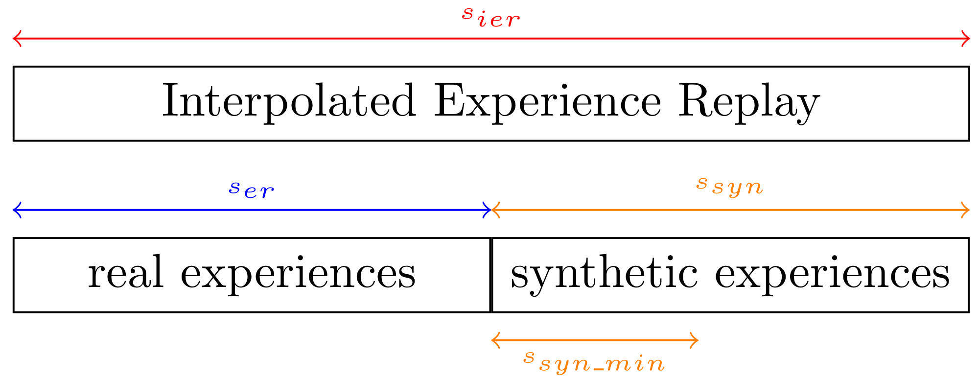
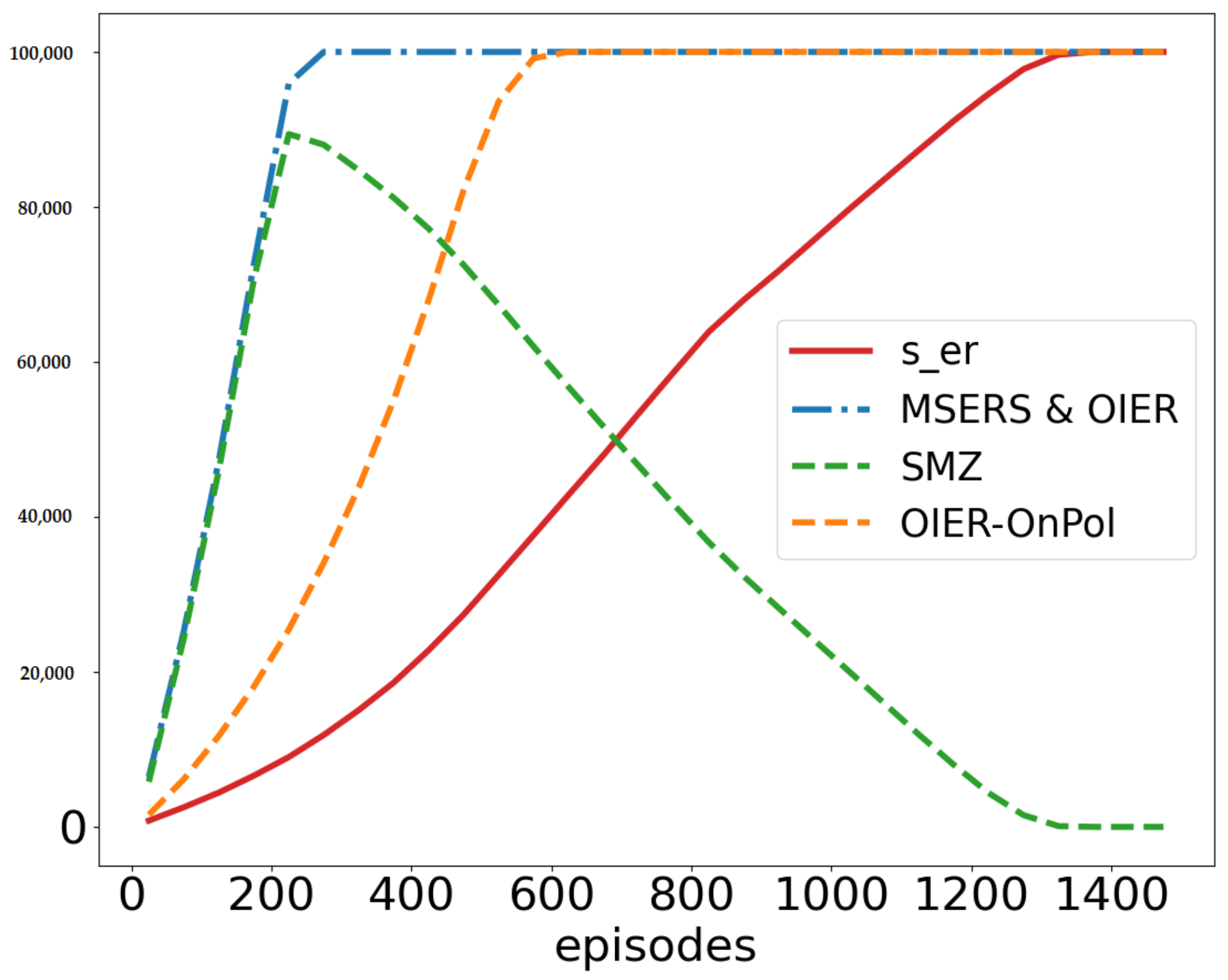
We replaced the SP with the ER. It is realized by a FiFo queue with a maximum length. This queue represents the classic ER and is filled only with real experiences. To store the synthetic transitions another queue, a so-called ShrinkingMemory is introduced. This second storage is characterized by its decreasing size. Starting at a predefined maximum, it gets smaller depending on the length of the real experience queue. The Interpolated Experience Replay (IER) has a total size, comprising the sum of the lengths of both queues, as can be seen in Figure 3. If this size is reached, the length of the ShrinkingMemory is decreased, and the oldest items are removed. This goes on as long as either the real valued queue reaches its maximum length and there is some space left for interpolated experiences or the IER fills up with real experiences. As interpolation is a lot of extra work, it might seem counterproductive to throw such examples away, but this decision was made because of two reasons:
- As the learner comes near convergence, randomly distributed experiences might harm the real distribution that is derived by following the actual policy. Following this point, the learner benefits more from real experiences as time goes by.
- The quality of the interpolated experiences is unclear and a bad interpolation could harm the learner even more than a misleading real experience. By throwing them away and regularly replacing them with new ones, we try to mitigate this effect.
We also introduced a minimum length for the interpolated storage that is never fallen below. This results in a differing behaviour from the above-explained procedure. If the ShrinkingMemory is instructed to reduce its length, it does this only until it reaches this threshold. Therefore, the maximum length of the IER consists of the real experience buffers maximum length and the minimum length of the synthetic part .
The IER algorithm, as described in Section 4.2, is located in the Interpolant, and, as stated above, executed in every step. An exhaustive search would need a computation time of and therefore is not practical for large sized IERs because this operation is executed in every single step. A possible solution for this problem is to employ a so called kd-tree, which represents a multidimensional data structure. Using such a tree, the computation time could be decreased to [25]. As the examined problem is very small and consists out of discrete states, we use another approach to reduce the computation time further to . To achieve this, we use a dictionary of size with keys:
and corresponding values:
with:
This equals an entry for every state-action pair with associated average rewards and distinct next states of all seen transitions. The dictionary is updated after every transition the agent makes.
To evaluate the quality of computed interpolations, an appropriate metric cloud be used in the Evaluation part. This is not implemented yet and left for future work.
5. Evaluation
This chapter first introduces the experimental setup and is followed with a detailed evaluation of the results.
5.1. State Encodings
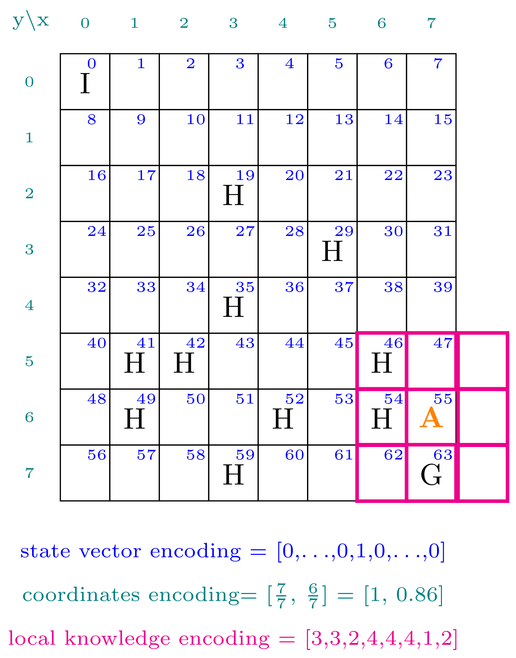
We investigated three different state encodings:
- State Vector Encoding (VE): The state vector encoding is realized with an array of the length of the state space (). The whole vector is filled with zeros, and the entry that corresponds to the actual state is set to 1. This results in an input layer of size 64.
- Coordinates Encoding (CE): The coordinates state encoding is realized via a vector with two entries that hold the value for the normalized x- and y-coordinate. An input layer of size two is used here.
- Local Knowledge Encoding (LKE): In the local knowledge state encoding, the agent receives a vector with eight entries that corresponds to the surrounding fields of the actual state. The different state types are shown in Table 1. We utilized an input layer of size 8. In this encoding, we face the problem of perceptual aliasing [26], as some states have the exact same encoding but in fact are different. These states share their collected follow-up states and rewards, and therefore, it is expected that a small real experience buffer should perform better than a big one because stored experiences are replaced with a higher frequency. Furthermore, the complexity of the problem increases because of these states.
A graphical illustration of the different encodings can be observed in Figure 4.
5.2. Query Methods
We investigated four different query methods of how to receive :
- Random (R): This method draws randomly from the state space. We expect this mode to assist the learner with exploration. Because the new inserted experiences induce a completely differing distribution (), this might also harm the learner. The concept is not feasible for LKE because the sampling of eight random numbers out of five possibilities results in illegal or not existing states most of the time.
- Policy Distribution (PD): This method draws a random state from the real experience buffer. The received state distribution resembles the one that is created by the policy. We expect the (possible) harmful effect of inducing a different sample distribution to be mitigated.
- Last State (LS): To stay even closer to the distribution created by the policy, this method takes the last state that was saved to the real experience buffer.
- Last State—On Policy Action Selection (LS-OnPol): In an attempt to stay even closer to the distribution that the policy creates, we use the LS query method in combination with an altered interpolation step. We only create synthetic experiences for one action that is given by the actual policy. Using this technique, we create synthetic samples for the same experiences the agent observed with a small deviation in the form of the actual of the exploration.
5.3. IER Modes
We investigated three different methods of how the IER was used:
- Synthetic Min Size Zero (MSZ): In this mode, we used a minimum size for the synthetic buffer of 0. In this configuration, the learner starts with a lot of synthetic samples in its buffer, but if he comes near convergence, they are replaced with real experiences, and in the end, the agent learns from the real data.
- Synthetic Min Size Equals Real Size (MSERS): In this mode, we set the to . The synthetic buffer fills up completely and stays like this. Overt time, the real experience buffer fills to the same size, and in the end, both buffers have the same length. This brings a ratio of synthetic to real experience samples in favour of the interpolated ones in the beginning and ends in an equal distribution of both.
- Only Use Interpolated Buffer (OIER): Because (as described in Section 4.2) we assume that our synthetic samples are even better than the real ones, we also investigated how our approach performs if we only train on them. The maximum length of the IER, in this case, is only related to because the real examples are never used for learning.
5.4. Hyperparameter
Preliminary experiments revealed the hyperparameters given in Table 2, which are shared by all experiments.
The used network architectures for the different state encodings are presented in Table 3. All networks use the same amount of output nodes.
Table 4 shows the different hyperparameter for the IER modes. The value of for OIER and MSERS varies for LKE from the other encodings and is much smaller; this comes from the assumption (as described in Section 5.1) that a smaller buffer would help to handle aliasing states because the rotation of the sampling points is increased that way. In contrast, we expect that a bigger buffer helps in the other cases because it corresponds to a bigger knowledge base and consequentially better synthetic experiences.
We used a linearly decaying -greedy as the exploration technique and investigated three different durations (500, 750 and 1000 episodes).
5.5. Experiments
As baseline, we used a DQN with vanilla ER and 100,000 for all three state encodings to compare the different configurations with.
The different constellations of the individual experiments are shown in Table 5. We measure the average return over the last 100 episodes to obtain a moving average that indicates how often the agent is able to reach the goal in this time. Each experiment was repeated 20 times, and the results are reported as the overall mean values and the observed standard deviations (SD) over the repetitions.
Each configuration was tested against the baseline, and the differences have been assessed for statistical significance. Therefore, we first conducted Shapiro–Wilk tests in conjunction with visual inspection of QQ-plots to determine whether a normal distribution can be assumed. Since this criterion could not be confirmed for any of the experiments, the Mann–Whitney-U test has been chosen. All measured statistics, comprising the corresponding p-values for the hypothesis tests, can be found in the Appendix A.
5.6. Experimental Results
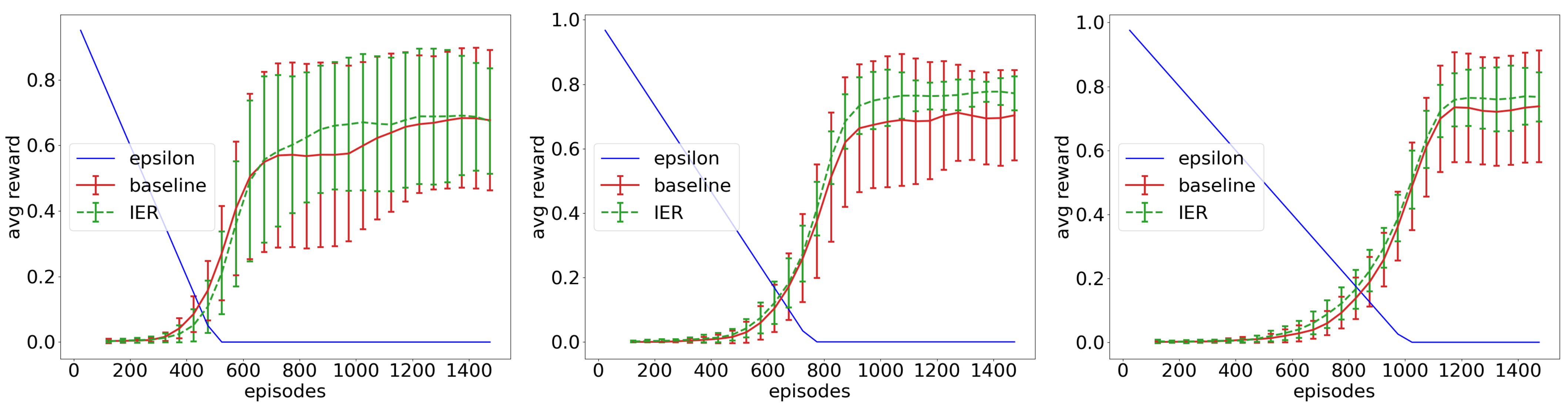
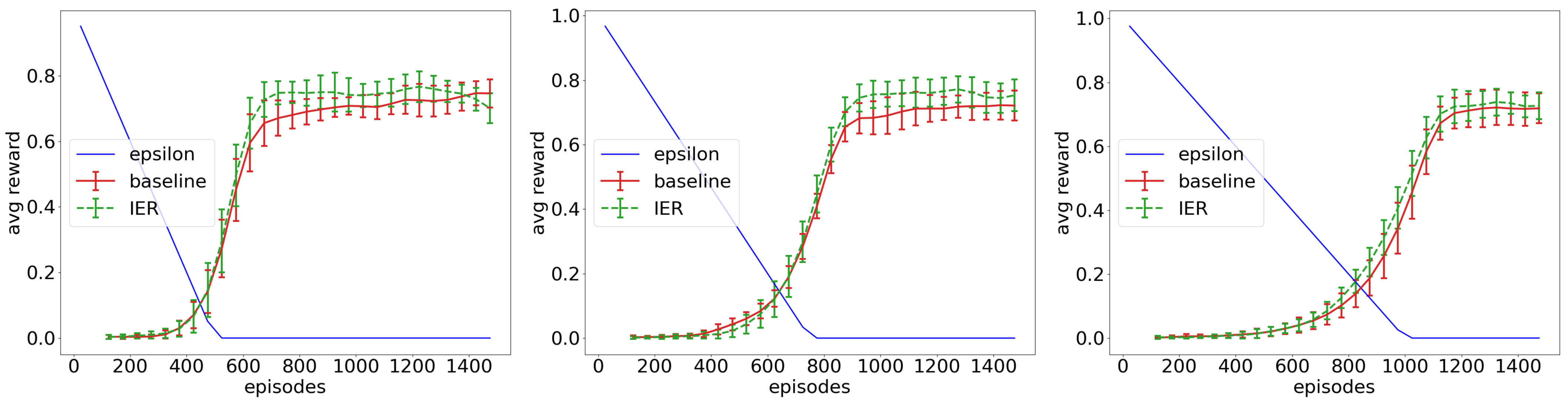
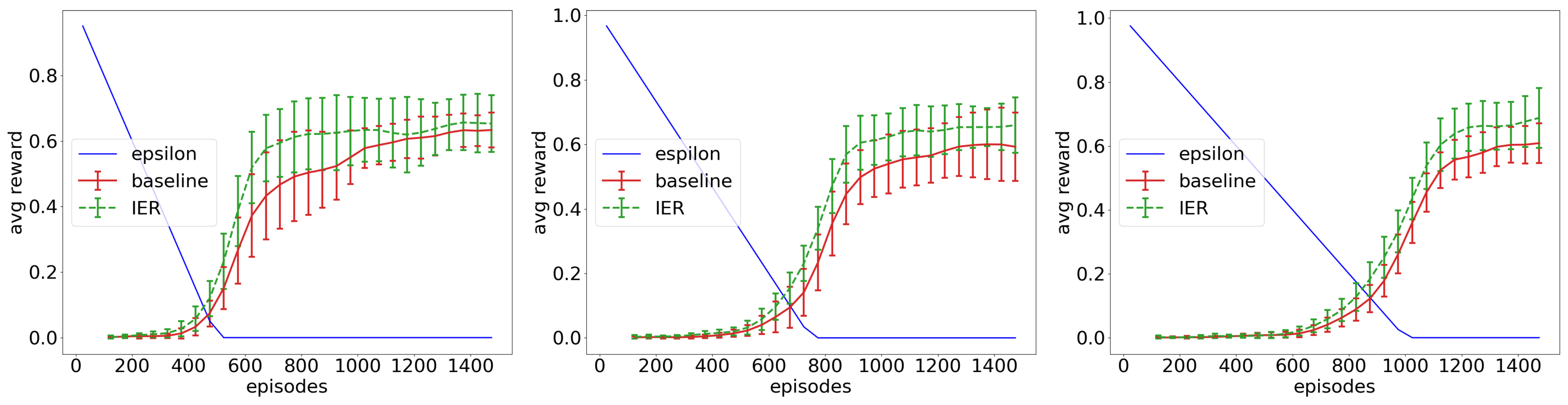
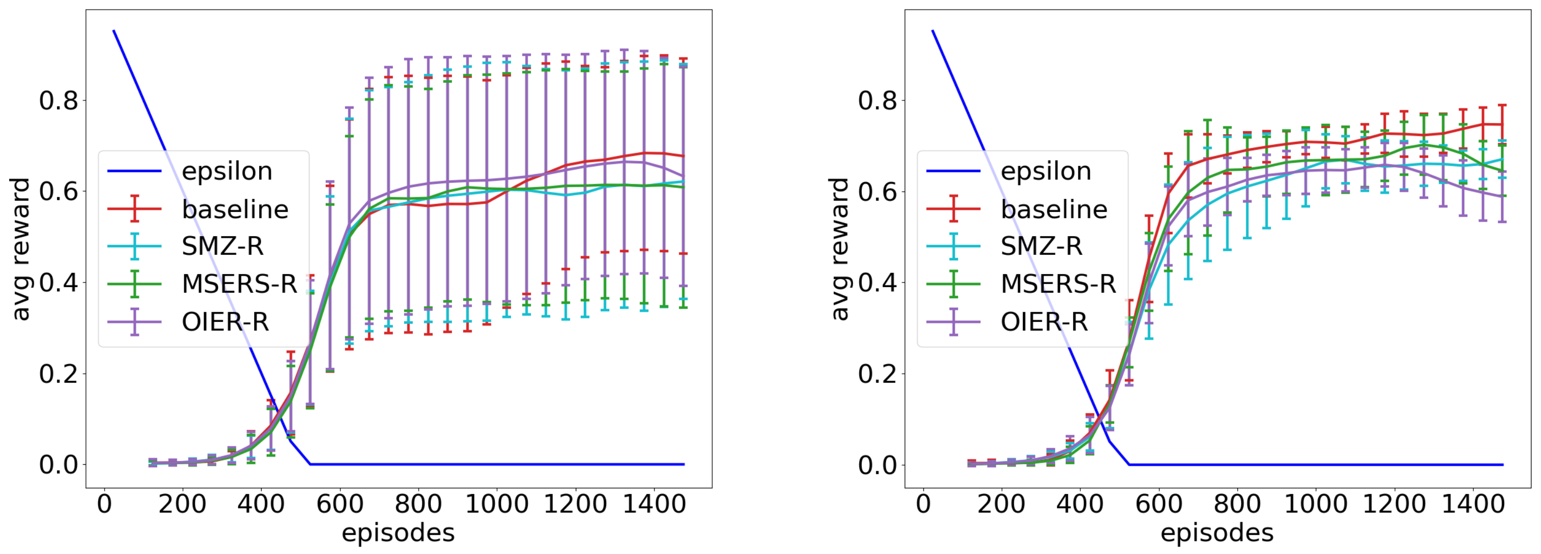
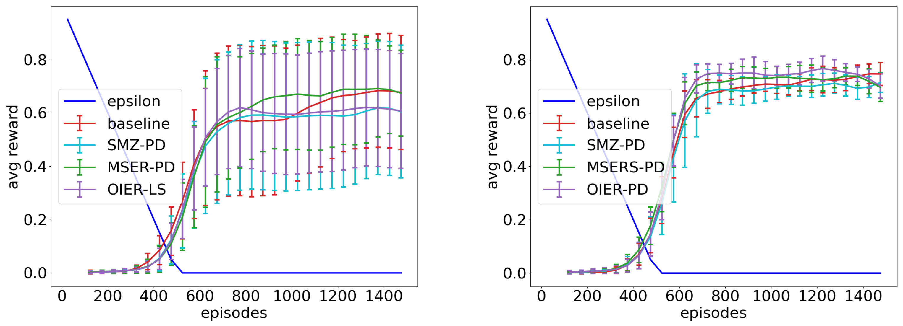
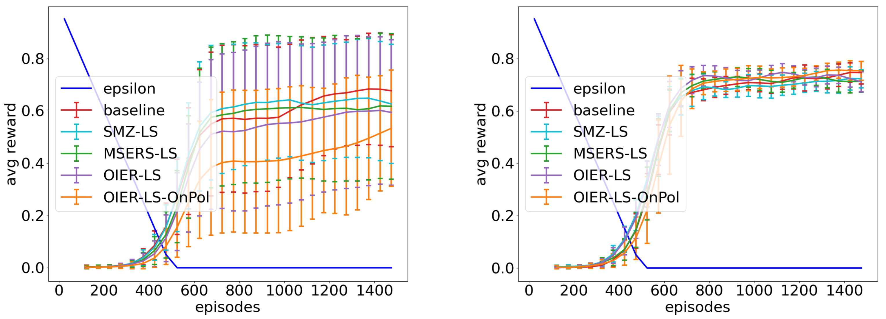
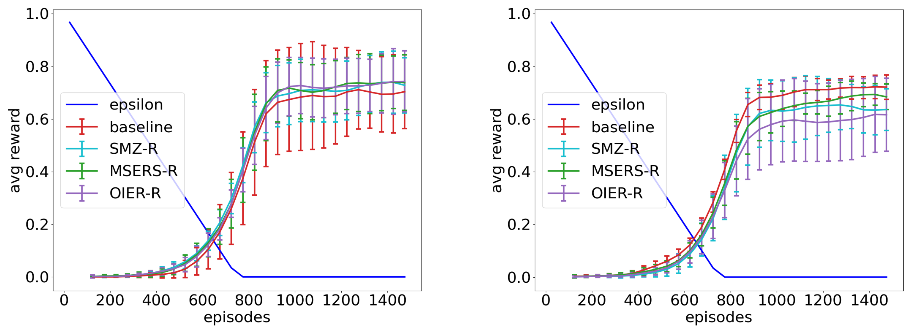
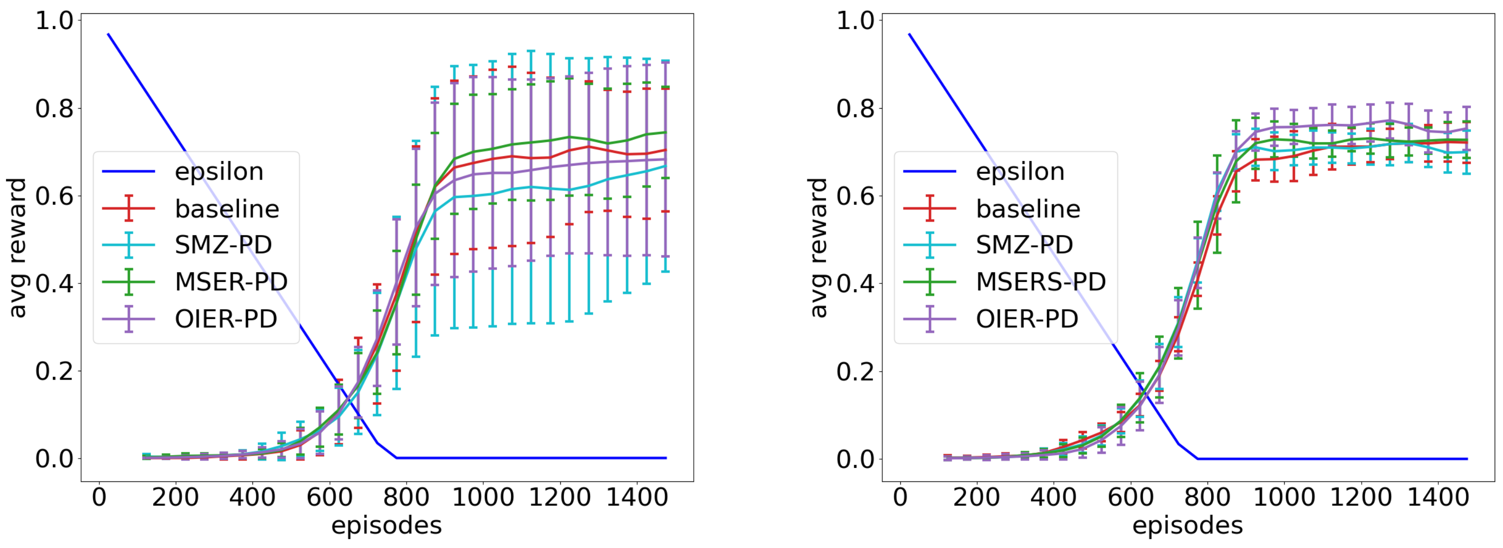
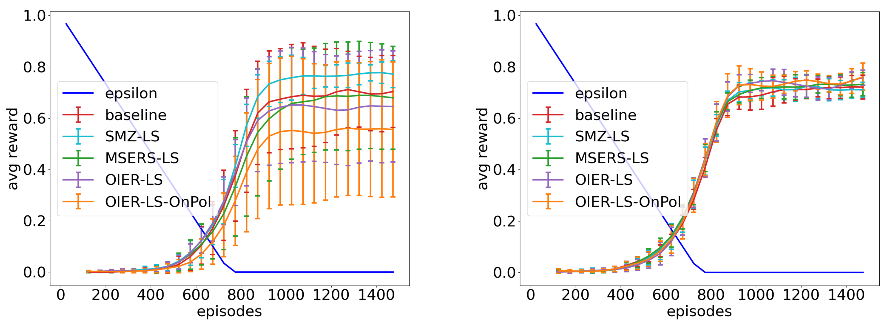
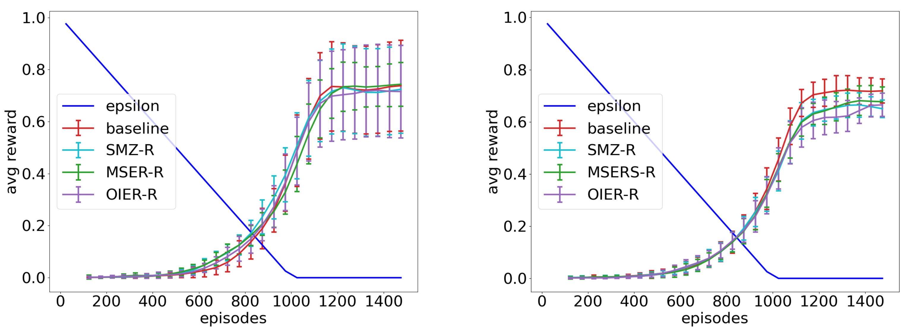
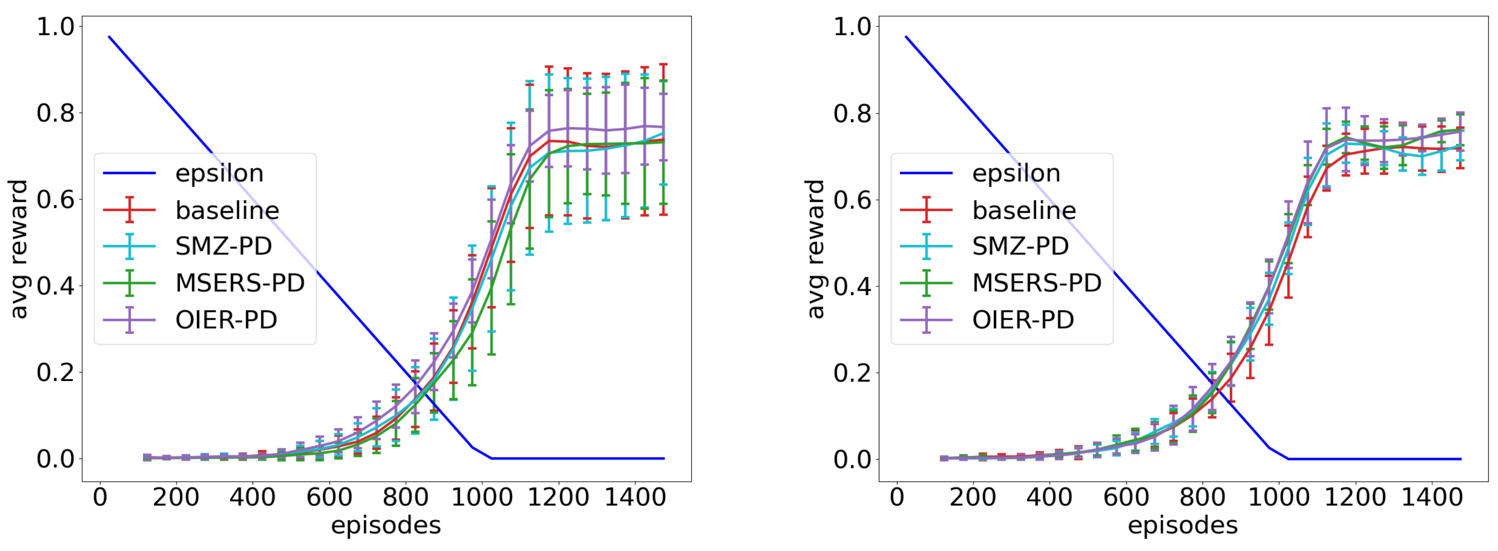
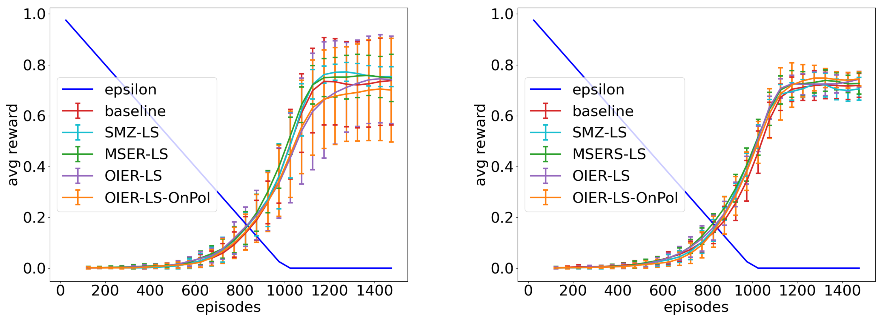
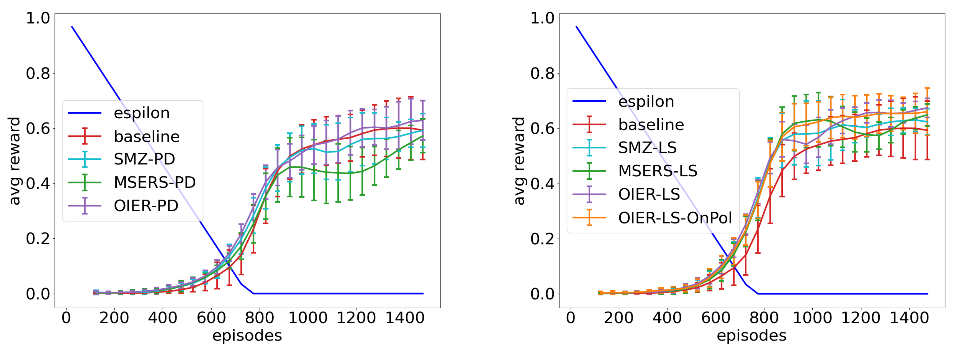
Figure 5, Figure 6 and Figure 7 depict the results of the best IER configurations, as given in Table 6. Each Figure holds the results for all investigated exploration phases in this order: . Figure 5 shows the result for the VE state encoding, Figure 6 the result for the CE state encoding and Figure 7 the result for the LKE state encoding. The graphs for all conducted experiments can be found in the Appendix B.
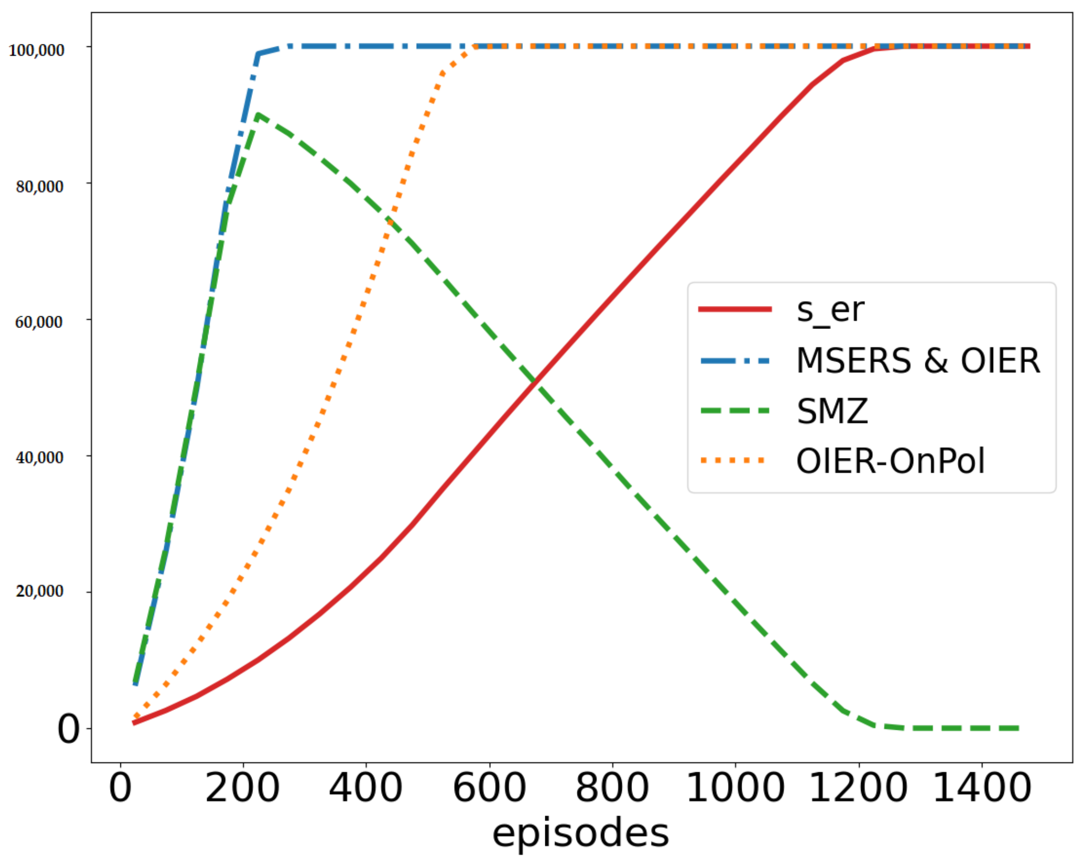
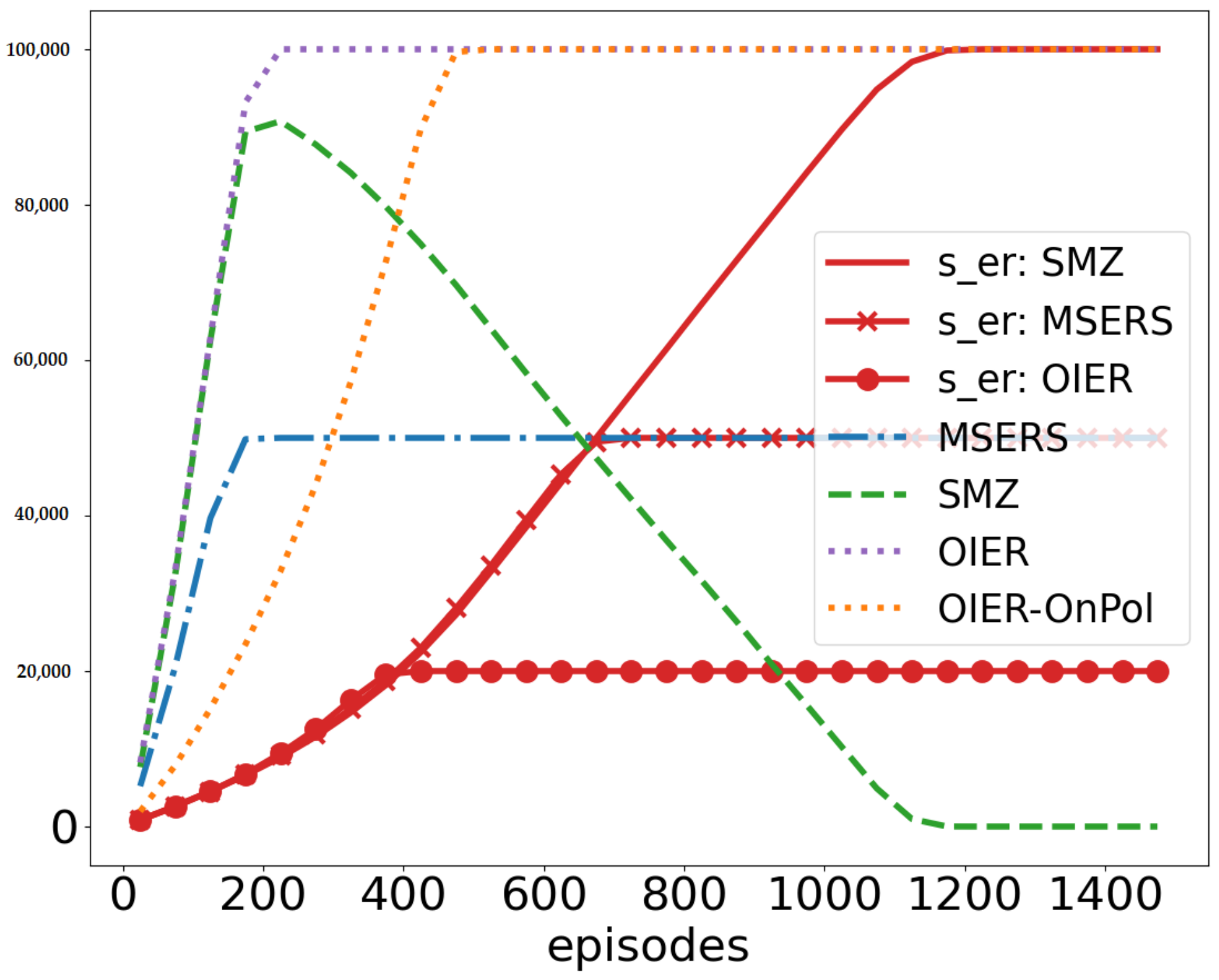
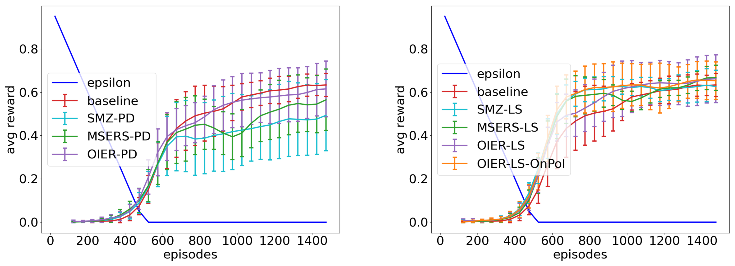
Figure 8, Figure 9 and Figure 10 picture the size of the IER at a given episode. As the graphs for different only differ marginally, we chose to present here. The graphs for experiment 1 and 2 look quite similar, but experiment 3 differs from them. This comes from the fact that we chose smaller values for for MSERS and OIER because of the aforementioned reasons. The orange curve, indicating OIER-OnPol, shows a less steep increase than the OIER configuration resulting from the creation of fewer synthetic samples.
5.7. Interpretation
All presented best configurations (Figure 5, Figure 6 and Figure 7) outperform their corresponding baseline (red line) and converge on a higher value alongside a steeper increase. This effect even increases with a smaller value of . The IER approach and the baseline for remain close to each other after 1400 episodes, and we can expect a similar behaviour from the other experiments if we give them more time. This shows that our approach helps the agent to understand the underlying model of the environment in the early to mid stages of learning (exploration phase). This fits our expectations from Section 4.2, where we noted that will converge to after seeing enough samples, but our synthetic experiences can accelerate this process. The enhanced information encapsulated in a synthetic experience as well as the distribution created by the interpolation process help to reduce oscillations that come from the effect of shifting the Q-function away from .
The IER graph in Figure 6a ends slightly below the baseline. As it reaches a higher value, both overall and faster, we still consider it to outperform the baseline.
A closer look at Table 6 reveals a clear best configuration for experiment 3 (OIER-LS-OnPol). Experiment 2 favours OIER-PD with an outlier for , but the difference between OIER-PD and MSERS-LS is marginal here (cf. Appendix A), and therefore, we can declare OIER-PD as the best-performing configuration for this experiment. For the CE encoding, on the other hand, it is not as obvious, and we obtain three different configurations here. Overall, we can observe that the random query method performs poorly in comparison with the others, which fits our expectations from Section 5.2. The PD query method seems to be the most efficient method for encodings with global knowledge (VE and CE).
The agent limited to local knowledge benefited most from staying as close as possible to the distribution created by the policy. All interpolation techniques, except OnPol, create synthetic experiences for every action that has been performed from the actual state. A synthetic experience is created for every follow-up state that has been reached from this state-action-pair. This should result in a maximum of 12 created experiences for every state. In the case of conceptual aliasing, the agent observes more than three follow-up states, which leads to the creation of many synthetic experiences. This might harm the learner more than it helps. Reducing this amount (by only interpolating experiences for one action) helps the learner. Additionally, here comes the effect of a smaller value of into play because, as stored experiences are replaced more often, the used follow-up states for interpolation are located closer to the trajectory created by the policy, which results in lesser follow-up states for aliasing states.
The fact that the agents from experiment 1 and 2 do not benefit from the OnPol configuration could be explained by the bigger effect of exploration that is induced into the ER by interpolating all actions. This increased spread over the state space seems to assist the learner.
The best results can be observed in the LKE experiments. The problem of the conceptual aliasing that arises here brings an additional difficulty into play and complicates the whole learning process. Our synthetic experiences use the gathered problem knowledge stored in the real transitions and help the learner to understand the problem. As this fact holds for all state encodings, the LKE encoding benefits from the additional focus on promising follow-up states that are replicated in the ER (OnPol).
In conclusion, our approach outperforms the baseline in most of the configurations in every state encoding. Using only synthetic experiences and querying in a way that follows the policy distribution to some extend promises better results.
6. Conclusions and Future Work
We presented an extension for the classic ER used in Deep RL that includes synthetic experiences to speed up and improve learning in non-deterministic and discrete environments. The proposed algorithm interprets stored, actually experienced transitions as an (inaccurate) model of the environment and calculates synthetic -tuples by means of interpolation. The synthetic experiences comprise a more accurate estimate of the expected long-term return a state-action pair promises than a real transition does. We investigated three different state encodings of the FrozenLake8x8-v0 environment from the OpenAI Gym to evaluate our approach for varying network structures and different challenges. To date, the employed interpolation technique is a simple, equally weighted averaging that serves as an initial approach. More complex methods in even more complex problem spaces have to be investigated in the future. The IER approach was compared to the default ER in the FrozenLake8x8-v0 environment from the OpenAI Gym and showed an increased performance in terms of a 3–19% increased overall mean reward of the best-performing configurations. By the investigation of different state encodings, query methods and IER modes, we were able to show that using only synthetic experiences and querying from the distribution created by the policy can assist the learner in terms of performance and speed.
As of yet, the proposed approach is limited to discrete and nondeterministic environments. We plan to develop the IER further to solve more complex problems (increased/continuous state and action space) as well. To achieve this, a solution for the unknown follow-up state is needed, which could also be interpolated or even predicted by a state-transition function that is learned in parallel. Here, the work from [18] could serve as a possible approach to begin with. A simple, yet nevertheless, more complex problem because of its continuity that is beyond the domain of grid worlds is the MountainCar problem. Other, more complex interpolation techniques have to be examined to adapt our IER approach in this environment. Furthermore, at last, the impact of interpolated experiences on more sophisticated Experience Replay mechanisms, such as Hindsight ER and Prioritized ER, have to be investigated as well.
Author Contributions
Conceptualization, W.P.v.P. and A.S.; methodology, W.P.v.P. and A.S.; software, W.P.v.P.; validation, W.P.v.P. and A.S.; resources, J.H.; writing—original draft preparation, W.P.v.P.; writing—review and editing, A.S. and J.H.; visualization, W.P.v.P.; supervision, J.H. and A.S. All authors have read and agreed to the published version of the manuscript.
Funding
This research received no external funding.
Institutional Review Board Statement
Not applicable.
Informed Consent Statement
Not applicable.
Data Availability Statement
Not applicable.
Conflicts of Interest
The authors declare no conflict of interest.
Abbreviations
The following abbreviations are used in this manuscript:
| RL | Reinforcement Learning |
| DQN | Deep Q-Network |
| ER | Experience Replay |
| IC | Interpolation Component |
| MLI | Machine Learning Interface |
| SP | Sampling Points |
| IER | Interpolated Experience Replay |
| VE | State Vector Encoding |
| CE | Coordinates Encoding |
| LKE | Local Knowledge Encoding |
| R | Random |
| PD | Policy Distribution |
| LS | Last State |
| LS-OnPol | Last State-On Policy Action Selection |
| SMZ | Synthetic Min Size Zero |
| SMERS | Synthetic Min Size Equals Real Size |
| OIER | Only Use Interpolated Buffer |
Appendix A

Table A1.
A summary of the results of experiment 1 with state-encoding VE. Bold mean entries show a better performance in comparison to the corresponding baseline; bold IER-Query- entries indicate statistically significant superior performance compared to the baseline.
Table A1.
A summary of the results of experiment 1 with state-encoding VE. Bold mean entries show a better performance in comparison to the corresponding baseline; bold IER-Query- entries indicate statistically significant superior performance compared to the baseline.
| IER-Query- | Mean | ±1SD | p-Value | p-Value |
|---|---|---|---|---|
| Shapiro–Wilk | Mann–Whitney-U | |||
| baseline-500 | 0.4111 | ±0.2629 | 1.9602 × 10 | |
| SMZ-R-500 | 0.3983 | ±0.2529 | 4.4099 × 10 | 0.0286 |
| SMZ-PD-500 | 0.3885 | ±0.254 | 5.5603 × 10 | 0.0045 |
| SMZ-LS-500 | 0.423 | ±0.2694 | 2.2323 × 10 | 0.0017 |
| MSERS-R-500 | 0.4007 | ±0.2577 | 2.2673 × 10 | 0.1916 |
| MSERS-PD-500 | 0.4252 | ±0.2862 | 2.6488 × 10 | 3.6207 × 10 |
| MSERS-LS-500 | 0.4015 | ±0.2603 | 5.7874 × 10 | 0.4342 |
| OIER-R-500 | 0.4222 | ±0.2696 | 3.5167 × 10 | 0.0004 |
| OIER-PD-500 | 0.4011 | ±0.2624 | 1.058 × 10 | 0.3721 |
| OIER-LS-500 | 0.3685 | ±0.2414 | 2.906 × 10 | 2.4301 × 10 |
| OIER-LS-OnPol-500 | 0.2825 | ±0.1881 | 1.4649 × 10 | 1.0855 × 10 |
| baseline-750 | 0.3484 | ±0.3100 | 1.2353 × 10 | |
| SMZ-R-750 | 0.3713 | ±0.3160 | 3.8829 × 10 | 3.4641 × 10 |
| SMZ-PD-750 | 0.316 | ±0.2757 | 2.3740 × 10 | 1.4685 × 10 |
| SMZ-LS-750 | 0.3862 | ±0.341 | 7.0165 × 10 | 8.3487 × 10 |
| MSERS-R-750 | 0.3706 | ±0.3208 | 2.1825 × 10 | 1.0342 × 10 |
| MSERS-PD-750 | 0.3583 | ±0.3198 | 1.4494 × 10 | 9.3729 × 10 |
| MSERS-LS-750 | 0.3319 | ±0.2962 | 1.6246 × 10 | 0.0014 |
| OIER-R-750 | 0.3691 | ±0.3212 | 1.3013 × 10 | 1.4234 × 10 |
| OIER-PD-750 | 0.3396 | ±0.2971 | 9.2585 × 10 | 1.9481 × 10 |
| OIER-LS-750 | 0.3329 | ±0.2858 | 9.8819 × 10 | 7.0010 × 10 |
| OIER-LS-OnPol-750 | 0.2734 | ±0.2473 | 4.6952 × 10 | 1.0123 × 10 |
| baseline-1k | 0.2564 | ±0.2981 | 1.5026 × 10 | |
| SMZ-R-1k | 0.2666 | ±0.2910 | 6.691 × 10 | 0.1832 |
| SMZ-PD-1k | 0.2514 | ±0.2894 | 3.7812 × 10 | 0.2072 |
| SMZ-LS-1k | 0.2676 | ±0.3107 | 3.6418 × 10 | 0.1699 |
| MSERS-R-1k | 0.2574 | ±0.2866 | 6.8941 × 10 | 0.0011 |
| MSERS-PD-1k | 0.2395 | ±0.2892 | 1.0053 × 10 | 0.0044 |
| MSERS-LS-1k | 0.2728 | ±0.3076 | 5.3421 × 10 | 1.3641 × 10 |
| OIER-R-1k | 0.2567 | ±0.2878 | 1.1493 × 10 | 0.4688 |
| OIER-PD-1k | 0.2747 | ±0.3084 | 1.1251 × 10 | 3.7636 × 10 |
| OIER-LS-1k | 0.2481 | ±0.28 | 2.0074 × 10 | 0.3419 |
| OIER-LS-OnPol-1k | 0.2416 | ±0.2769 | 1.2080 × 10 | 0.001 |
Table A2.
A summary of the results of experiment 2 with state-encoding CE. Bold mean entries show a better performance in comparison to the corresponding baseline; bold IER-Query- entries indicate statistically significant superior performance compared to the baseline.
Table A2.
A summary of the results of experiment 2 with state-encoding CE. Bold mean entries show a better performance in comparison to the corresponding baseline; bold IER-Query- entries indicate statistically significant superior performance compared to the baseline.
| IER-Query- | Mean | ±1SD | p-Value | p-Value |
|---|---|---|---|---|
| Shapiro–Wilk | Mann–Whitney-U | |||
| baseline-500 | 0.4677 | ±0.3060 | 5.3488 × 10 | |
| SMZ-R-500 | 0.4180 | ±0.2747 | 2.6105 × 10 | 3.2958 × 10 |
| SMZ-PD-500 | 0.4579 | ±0.2998 | 1.3438 × 10 | 4.33597 × 10 |
| SMZ-LS-500 | 0.4722 | ±0.2930 | 2.3623× 10 | 0.0002 |
| MSERS-R-500 | 0.4394 | ±0.2895 | 1.8445 × 10 | 8.3967 × 10 |
| MSERS-PD-500 | 0.4885 | ±0.3116 | 3.6434 × 10 | 1.5353 × 10 |
| MSERS-LS-500 | 0.4759 | ±0.3092 | 9.9072 × 10 | 1.3453 × 10 |
| OIER-R-500 | 0.4186 | ±0.2725 | 1.1939 × 10 | 1.1663 × 10 |
| OIER-PD-500 | 0.4983 | ±0.3252 | 2.13 × 10 | 6.0368 × 10 |
| OIER-LS-500 | 0.4896 | ±0.3102 | 1.7278 × 10 | 7.0417 × 10 |
| OIER-LS-OnPol-500 | 0.469 | ±0.3161 | 1.4621 × 10 | 5.8208 × 10 |
| baseline-750 | 0.3661 | ±0.3128 | 2.003 × 10 | |
| SMZ-R-750 | 0.3218 | ±0.2880 | 5.0337 × 10 | 1.3713 × 10 |
| SMZ-PD-750 | 0.3750 | ±0.3182 | 2.5529 × 10 | 0.4158 |
| SMZ-LS-750 | 0.3733 | ±0.3167 | 9.6999 × 10 | 0.0290 |
| MSERS-R-750 | 0.3339 | ±0.2926 | 1.4778 × 10 | 4.0643 × 10 |
| MSERS-PD-750 | 0.3779 | ±0.3227 | 5.3906 × 10 | 2.2138 × 10 |
| MSERS-LS-750 | 0.3776 | ±0.3188 | 2.1208 × 10 | 2.1575 × 10 |
| OIER-R-750 | 0.301 | ±0.2628 | 1.9892 × 10 | 9.0174 × 10 |
| OIER-PD-750 | 0.3894 | ±0.3408 | 3.4510 × 10 | 5.8499 × 10 |
| OIER-LS-750 | 0.3791 | ±0.3269 | 6.819 × 10 | 5.6256 × 10 |
| OIER-LS-OnPol-750 | 0.3816 | ±0.3273 | 6.0862 × 10 | 2.0991 × 10 |
| baseline-1k | 0.2533 | ±0.2875 | 5.5541 × 10 | |
| SMZ-R-1k | 0.2344 | ±0.2604 | 3.9105 × 10 | 0.0076 |
| SMZ-PD-1k | 0.2619 | ±0.2921 | 1.6130 × 10 | 0.3994 |
| SMZ-LS-1k | 0.2607 | ±0.2928 | 7.2215 × 10 | 0.0418 |
| MSERS-R-1k | 0.2333 | ±0.2630 | 3.5365 × 10 | 0.0006 |
| MSERS-PD-1k | 0.2688 | ±0.3001 | 9.5744 × 10 | 0.0643 |
| MSERS-LS-1k | 0.2707 | ±0.2975 | 2.713 × 10 | 0.0389 |
| OIER-R-1k | 0.2263 | ±0.2497 | 8.275 × 10 | 2.8409 × 10 |
| OIER-PD-1k | 0.2704 | ±0.3023 | 7.0418 × 10 | 0.0974 |
| OIER-LS-1k | 0.2656 | ±0.2965 | 6.2867 × 10 | 0.1209 |
| OIER-LS-OnPol-1k | 0.2607 | ±0.3011 | 3.7218 × 10 | 0.2205 |
Table A3.
A summary of the results of experiment 3 with state-encoding LKE. Bold mean entries show a better performance in comparison to the corresponding baseline; bold IER-Query- entries indicate statistically significant superior performance compared to the baseline.
Table A3.
A summary of the results of experiment 3 with state-encoding LKE. Bold mean entries show a better performance in comparison to the corresponding baseline; bold IER-Query- entries indicate statistically significant superior performance compared to the baseline.
| IER-Query- | Mean | ±1SD | p-Value | p-Value |
|---|---|---|---|---|
| Shapiro–Wilk | Mann–Whitney-U | |||
| baseline-500 | 0.3562 | ±0.2503 | 4.8159 × 10 | |
| SMZ-PD-500 | 0.2846 | ±0.1859 | 1.6391 × 10 | 9.4865 × 10 |
| SMZ-LS-500 | 0.4072 | ±0.2648 | 2.4074 × 10 | 5.5843 × 10 |
| MSERS-PD-500 | 0.3092 | ±0.204 | 1.5363 × 10 | 5.3745 × 10 |
| MSERS-LS-500 | 0.3916 | ±0.2606 | 7.8533 × 10 | 1.4450 × 10 |
| OIER-PD-500 | 0.3551 | ±0.2352 | 1.5954 × 10 | 0.0227 |
| OIER-LS-500 | 0.3944 | ±0.2625 | 5.9815 × 10 | 1.5320 × 10 |
| OIER-LS-OnPol-500 | 0.4132 | ±0.2709 | 5.2100 × 10 | 6.4966 × 10 |
| baseline-750 | 0.2711 | ±0.2533 | 1.1861 × 10 | |
| SMZ-PD-750 | 0.2719 | ±0.2376 | 5.9007 × 10 | 0.4458 |
| SMZ-LS-750 | 0.3081 | ±0.2714 | 1.3309 × 10 | 4.3008 × 10 |
| MSERS-PD-750 | 0.2378 | ±0.2043 | 1.5783 × 10 | 2.2868 × 10 |
| MSERS-LS-750 | 0.3093 | ±0.2739 | 1.3558 × 10 | 1.1416 × 10 |
| OIER-PD-750 | 0.2871 | ±0.2489 | 1.0186 × 10 | 8.4356 × 10 |
| OIER-LS-750 | 0.3182 | ±0.2764 | 6.2019 × 10 | 1.4543 × 10 |
| OIER-LS-OnPol-750 | 0.3228 | ±0.2846 | 1.6222 × 10 | 7.6106 × 10 |
| baseline-1k | 0.1952 | ±0.2354 | 1.1519 × 10 | |
| SMZ-PD-1k | 0.1776 | ±0.1993 | 1.5132 × 10 | 0.1629 |
| SMZ-LS-1k | 0.2141 | ±0.2424 | 5.4984 × 10 | 3.4358 × 10 |
| MSERS-PD-1k | 0.1700 | ±0.1927 | 1.5335 × 10 | 0.4497 |
| MSERS-LS-1k | 0.224 | ±0.2619 | 1.7365 × 10 | 3.2996 × 10 |
| OIER-PD-1k | 0.1785 | ±0.2049 | 1.2643 × 10 | 0.3646 |
| OIER-LS-1k | 0.2099 | ±0.2354 | 4.9194 × 10 | 0.0042 |
| OIER-LS-OnPol-1k | 0.2311 | ±0.2670 | 4.4815 × 10 | 5.0054 × 10 |
Appendix B
Figure A1.
The results for the IER mode: R and . state encoding: VE. state encoding: CE.

Figure A2.
The results for the IER mode: PD and . state encoding: VE. state encoding: CE.

Figure A3.
The results for the IER mode: LS and . state encoding: VE. state encoding: CE.

Figure A4.
The results for the IER mode: R and . state encoding: VE. state encoding: CE.

Figure A5.
The results for the IER mode: PD and . state encoding: VE. state encoding: CE.

Figure A6.
The results for the IER mode: LS and . state encoding: VE. state encoding: CE.

Figure A7.
The results for the IER mode: R and . state encoding: VE. state encoding: CE.

Figure A8.
The results for the IER mode: PD and . state encoding: VE. state encoding: CE.

Figure A9.
The results for the IER mode: LS and . state encoding: VE. state encoding: CE.

Figure A10.
The results and state encoding for: LKE and IER mode: PD. . .

Figure A11.
The results for state encoding: LKE. IER mode: PD and . IER mode: LS and .

Figure A12.
The results for state encoding: LKE and IER mode: LS. . .

References
- Schaul, T.; Quan, J.; Antonoglou, I.; Silver, D. Prioritized Experience Replay. arXiv 2015, arXiv:1511.05952. [Google Scholar]
- Mnih, V.; Kavukcuoglu, K.; Silver, D.; Rusu, A.A.; Veness, J.; Bellemare, M.G.; Graves, A.; Riedmiller, M.; Fidjeland, A.K.; Ostrovski, G.; et al. Human-level control through deep reinforcement learning. Nature 2015, 518, 529. [Google Scholar] [CrossRef] [PubMed]
- Andrychowicz, M.; Wolski, F.; Ray, A.; Schneider, J.; Fong, R.; Welinder, P.; McGrew, B.; Tobin, J.; Abbeel, P.; Zaremba, W. Hindsight Experience Replay. In Advances in Neural Information Processing Systems 30; Curran Associates, Inc.: Red Hook, NY, USA, 2017; pp. 5048–5058. [Google Scholar]
- Lin, L.J. Self-improving reactive agents based on reinforcement learning, planning and teaching. Mach. Learn. 1992, 8, 293–321. [Google Scholar] [CrossRef]
- Tsitsiklis, J.N.; Roy, B.V. An analysis of temporal-difference learning with function approximation. IEEE Trans. Autom. Control 1997, 42, 674–690. [Google Scholar] [CrossRef] [Green Version]
- Zhang, S.; Sutton, R.S. A Deeper Look at Experience Replay. arXiv 2017, arXiv:1712.01275. [Google Scholar]
- Brockman, G.; Cheung, V.; Pettersson, L.; Schneider, J.; Schulman, J.; Tang, J.; Zaremba, W. OpenAI Gym. arXiv 2016, arXiv:1606.01540. [Google Scholar]
- Von Pilchau, W.B.P.; Stein, A.; Hähner, J. Bootstrapping a DQN replay memory with synthetic experiences. In Proceedings of the 12th International Joint Conference on Computational Intelligence (IJCCI 2020), Budapest, Hungary, 2–4 November 2020. [Google Scholar] [CrossRef]
- McClelland, J.L.; McNaughton, B.L.; O’Reilly, R.C. Why there are complementary learning systems in the hippocampus and neocortex: Insights from the successes and failures of connectionist models of learning and memory. Psychol. Rev. 1995, 102, 419. [Google Scholar] [CrossRef] [PubMed] [Green Version]
- O’Neill, J.; Pleydell-Bouverie, B.; Dupret, D.; Csicsvari, J. Play it again: Reactivation of waking experience and memory. Trends Neurosci. 2010, 33, 220–229. [Google Scholar] [CrossRef] [PubMed]
- Lin, L.J. Reinforcement Learning for Robots Using Neural Networks; Technical Report; Carnegie-Mellon Univ Pittsburgh PA School of Computer Science: Pittsburgh, PA, USA, 1993. [Google Scholar]
- Sutton, R.S.; Barto, A.G. Reinforcement Learning: An Introduction; MIT Press: Cambridge, MA, USA, 2018. [Google Scholar]
- Watkins, C.J.C.H.; Dayan, P. Q-learning. Mach. Learn. 1992, 8, 279–292. [Google Scholar] [CrossRef]
- Mnih, V.; Kavukcuoglu, K.; Silver, D.; Graves, A.; Antonoglou, I.; Wierstra, D.; Riedmiller, M.A. Playing Atari with Deep Reinforcement Learning. arXiv 2013, arXiv:1312.5602. [Google Scholar]
- Lillicrap, T.P.; Hunt, J.J.; Pritzel, A.; Heess, N.; Erez, T.; Tassa, Y.; Silver, D.; Wierstra, D. Continuous control with deep reinforcement learning. In Proceedings of the 4th International Conference on Learning Representations, ICLR 2016, San Juan, Puerto Rico, 2–4 May 2016. [Google Scholar]
- De Bruin, T.; Kober, J.; Tuyls, K.; Babuška, R. The importance of experience replay database composition in deep reinforcement learning. In Proceedings of the Deep Reinforcement Learning Workshop, Montréal, QC, Canada, 11 December 2015. [Google Scholar]
- de Bruin, T.; Kober, J.; Tuyls, K.; Babuška, R. Improved deep reinforcement learning for robotics through distribution-based experience retention. In Proceedings of the 2016 IEEE/RSJ International Conference on Intelligent Robots and Systems (IROS), Daejeon, Korea, 9–14 October 2016; pp. 3947–3952. [Google Scholar] [CrossRef] [Green Version]
- Jiang, W.; Hwang, K.; Lin, J. An Experience Replay Method based on Tree Structure for Reinforcement Learning. IEEE Trans. Emerg. Top. Comput. 2019, 9, 972–982. [Google Scholar] [CrossRef]
- Gu, S.S.; Lillicrap, T.; Turner, R.E.; Ghahramani, Z.; Schölkopf, B.; Levine, S. Interpolated policy gradient: Merging on-policy and off-policy gradient estimation for deep reinforcement learning. arXiv 2017, arXiv:1706.00387. [Google Scholar]
- Stein, A.; Rauh, D.; Tomforde, S.; Hähner, J. Augmenting the Algorithmic Structure of XCS by Means of Interpolation. In Architecture of Computing Systems—ARCS 2016; Hannig, F., Cardoso, J.M.P., Pionteck, T., Fey, D., Schröder-Preikschat, W., Teich, J., Eds.; Springer International Publishing: Cham, Switzerland, 2016; pp. 348–360. [Google Scholar]
- Stein, A.; Tomforde, S.; Rauh, D.; Hähner, J. Dealing with Unforeseen Situations in the Context of Self-Adaptive Urban Traffic Control: How to Bridge the Gap? In Proceedings of the 2016 IEEE International Conference on Autonomic Computing (ICAC), Wuerzburg, Germany, 17–22 July 2016. [Google Scholar]
- Stein, A.; Rauh, D.; Tomforde, S.; Hähner, J. Interpolation in the eXtended Classifier System: An architectural perspective. J. Syst. Archit. 2017, 75, 79–94. [Google Scholar] [CrossRef]
- Stein, A.; Menssen, S.; Hähner, J. What about Interpolation? A Radial Basis Function Approach to Classifier Prediction Modeling in XCSF. In Proceedings of the Genetic and Evolutionary Computation Conference GECCO ’18, Kyoto, Japan, 15–19 July 2018; Association for Computing Machinery: New York, NY, USA, 2018; pp. 537–544. [Google Scholar] [CrossRef]
- Stein, A.; Eymüller, C.; Rauh, D.; Tomforde, S.; Hähner, J. Interpolation-based classifier generation in XCSF. In Proceedings of the 2016 IEEE Congress on Evolutionary Computation (CEC), Vancouver, BC, Canada, 24–29 July 2016; pp. 3990–3998. [Google Scholar] [CrossRef]
- Friedman, J.H.; Bentley, J.L.; Finkel, R.A. An algorithm for finding best matches in logarithmic expected time. ACM Trans. Math. Softw. (TOMS) 1977, 3, 209–226. [Google Scholar] [CrossRef]
- Whitehead, S.D.; Ballard, D.H. Learning to perceive and act by trial and error. Mach. Learn. 1991, 7, 45–83. [Google Scholar] [CrossRef] [Green Version]
Figure 1.
The FrozenLake8x8-v0 environment from OpenAI Gym [7].
Figure 1.
The FrozenLake8x8-v0 environment from OpenAI Gym [7].

Figure 2.
A schematic of the Interpolation Component from Stein et al. [22].
Figure 2.
A schematic of the Interpolation Component from Stein et al. [22].

Figure 3.
Intuition of Interpolated Experience Replay memory.

Figure 4.
A graphical illustration of the three different state encodings. Every tile is represented by an index for the VE encoding. A coordinate system is used for the CE encoding and the surrounding 8 tiles represent the LKE encoding. An example for the state A is given for every encoding in the bottom.

Figure 5.
The best results among all conducted experiments with state-encoding VE. The solid red line represents the classical ER serving as baseline to compare with. The dashed green line shows the average reward of the IER approach. The blue line depicts the decaying epsilon. The lines for IER and the baseline represent the repetition averages. . . .

Figure 6.
The best results among all conducted experiments with state-encoding CE. The solid red line represents the classical ER serving as baseline to compare with. The dashed green line shows the average reward of the IER approach. The blue line depicts the decaying epsilon. The lines for IER and the baseline represent the repetition averages. . . .

Figure 7.
The best results among all conducted experiments with state-encoding LKE. The solid red line represents the classical ER serving as baseline to compare with. The dashed green line shows the average reward of the IER approach. The blue line depicts the decaying epsilon. The lines for IER and the baseline represent the repetition averages. . . .

Figure 8.
The intuition of Interpolated Experience Replay memory for the VE state encoding and .

Figure 9.
THe intuition of Interpolated Experience Replay memory for the CE state encoding and .

Figure 10.
The intuition of Interpolated Experience Replay memory for the LKE state encoding and .

Table 1.
An overview of the values for the different types of tiles in the LKE state encoding.
| Tile Type | Value |
|---|---|
| initial state | 0 |
| final state | 1 |
| frozen | 2 |
| hole | 3 |
| out of state space | 4 |
Table 2.
An overview of hyperparameters applied for the FrozenLake8x8-v0 experiment.
| Parameter | Value |
|---|---|
| Learning rate | 0.0005 |
| Discount factor | 0.95 |
| Epsilon start | 1 |
| Epsilon min | 0 |
| soft replacement | 0.25 |
| Size of IER | 100k |
| Start Learning at size of IER | 200 |
| Minibatch size | 32 |
| Start interpolation at | 100 |
| double | True |
| dueling | True |
Table 3.
The used network architectures for the different state encodings.
| State Encoding | Input | Hidden Layer | Output |
|---|---|---|---|
| VE | 64 | [32, 32] | 4 |
| CE | 2 | [128, 256] | 4 |
| LKE | 8 | [64, 64] | 4 |
Table 4.
The IER-related hyperparameter for the different IER modes.
| IER Mode | State Encoding | |IER| | ||
|---|---|---|---|---|
| MSZ | All | 100 k | 0 | 100 k |
| MSERS | VE and CE | 100 k | 100 k | 200 k |
| LKE | 50 k | 50 k | 100 k | |
| OIER | VE and CE | 100 k | 100 k | 100 k |
| LKE | 20k |
Table 5.
An overview of the individually conducted experiment constellations.
| Experiment | State Encoding | IER Mode | Query Method | |||
|---|---|---|---|---|---|---|
| 1 | VE | SMZ | × | R | 500 | |
| MSERS | PD | × | 750 | |||
| OIER | LS | 1 k | ||||
| OIER | LS-OnPol | |||||
| 2 | CE | SMZ | × | R | 500 | |
| MSERS | PD | × | 750 | |||
| OIER | LS | 1 k | ||||
| OIER | LS-OnPol | |||||
| 3 | LKE | SMZ | × | 500 | ||
| MSERS | PD | × | 750 | |||
| OIER | LS | 1 k | ||||
| OIER | LS-OnPol |
Table 6.
Best IER configurations found during the evaluation. The last two columns depict the overall received mean reward of the configuration and its corresponding baseline. A higher value indicates better performance.
Table 6.
Best IER configurations found during the evaluation. The last two columns depict the overall received mean reward of the configuration and its corresponding baseline. A higher value indicates better performance.
| Experiment | State Encoding | Configuration | Mean | Mean | |
|---|---|---|---|---|---|
| Baseline | Config | ||||
| 1 | VE | 500 | MSERS-PD | 0.4111 | 0.4252 |
| 750 | SMZ-LS | 0.3484 | 0.3862 | ||
| 1000 | OIER-PD | 0.2564 | 0.2747 | ||
| 2 | CE | 500 | OIER-PD | 0.4677 | 0.4983 |
| 750 | OIER-PD | 0.3661 | 0.3894 | ||
| 1000 | MSERS-LS | 0.2533 | 0.2707 | ||
| 3 | LKE | 500 | OIER-LS-OnPol | 0.3562 | 0.4132 |
| 750 | OIER-LS-OnPol | 0.2711 | 0.3228 | ||
| 1000 | OIER-LS-OnPol | 0.1952 | 0.2311 |
Publisher’s Note: MDPI stays neutral with regard to jurisdictional claims in published maps and institutional affiliations. |
© 2021 by the authors. Licensee MDPI, Basel, Switzerland. This article is an open access article distributed under the terms and conditions of the Creative Commons Attribution (CC BY) license (https://creativecommons.org/licenses/by/4.0/).
Share and Cite
MDPI and ACS Style
Pilar von Pilchau, W.; Stein, A.; Hähner, J. Synthetic Experiences for Accelerating DQN Performance in Discrete Non-Deterministic Environments. Algorithms 2021, 14, 226. https://0-doi-org.brum.beds.ac.uk/10.3390/a14080226
AMA Style
Pilar von Pilchau W, Stein A, Hähner J. Synthetic Experiences for Accelerating DQN Performance in Discrete Non-Deterministic Environments. Algorithms. 2021; 14(8):226. https://0-doi-org.brum.beds.ac.uk/10.3390/a14080226
Chicago/Turabian StylePilar von Pilchau, Wenzel, Anthony Stein, and Jörg Hähner. 2021. "Synthetic Experiences for Accelerating DQN Performance in Discrete Non-Deterministic Environments" Algorithms 14, no. 8: 226. https://0-doi-org.brum.beds.ac.uk/10.3390/a14080226
Note that from the first issue of 2016, this journal uses article numbers instead of page numbers. See further details here.