
An Efficient Time-Variant Reliability Analysis Method with Mixed Uncertainties


1
Center for Research on Leading Technology of Special Equipment, School of Mechanical and Electric Engineering, Guangzhou University, Guangzhou 510006, China
2
Key Laboratory for Safety Control of Bridge Engineering, Ministry of Education and Hunan Province, Changsha University of Science and Technology, Changsha 410114, China
*
Authors to whom correspondence should be addressed.
Algorithms 2021, 14(8), 229; https://0-doi-org.brum.beds.ac.uk/10.3390/a14080229
Submission received: 17 June 2021
/
Revised: 27 July 2021
/
Accepted: 30 July 2021
/
Published: 31 July 2021
Abstract
:In practical engineering, due to the lack of information, it is impossible to accurately determine the distribution of all variables. Therefore, time-variant reliability problems with both random and interval variables may be encountered. However, this kind of problem usually involves a complex multilevel nested optimization problem, which leads to a substantial computational burden, and it is difficult to meet the requirements of complex engineering problem analysis. This study proposes a decoupling strategy to efficiently analyze the time-variant reliability based on the mixed uncertainty model. The interval variables are treated with independent random variables that are uniformly distributed in their respective intervals. Then the time-variant reliability-equivalent model, containing only random variables, is established, to avoid multi-layer nesting optimization. The stochastic process is first discretized to obtain several static limit state functions at different times. The time-variant reliability problem is changed into the conventional time-invariant system reliability problem. First order reliability analysis method (FORM) is used to analyze the reliability of each time. Thus, an efficient and robust convergence hybrid time-variant reliability calculation algorithm is proposed based on the equivalent model. Finally, numerical examples shows the effectiveness of the proposed method.
1. Introduction
Structural reliability is regarded as the ability of the device or structure to complete the required functions under the specified conditions within the prescribed design period [1,2,3,4,5]. Since the advent of this concept in engineering and industrial applications, structural reliability analysis in the probabilistic framework has been developed rapidly. Although a series of effective methods, including the first-order second-moment method [6,7], second-order second-moment method [8] and system reliability analysis [9], have been proposed. However, there are several time-variant uncertain parameters in practical structures such as external dynamic loads, degradation of material properties and changes of geometric characteristics that affect the time-variant reliability of structures [10]. Accordingly, it is significant importance to conduct to carry out a time-variant reliability analysis for the engineering structures.
Conventional time-variant reliability analyzing methods can be mainly divided into five categories [11,12,13], i.e. the first-passage method, numerical methods, extreme value density methods, surrogate methods and the quasi-static methods.
The time-variant reliability problem mainly originates from the first-passage method proposed by Rice [14] in the 1940s, which lays the foundation for the development of the subsequent crossing rate method. It should be noted that the calculation of the outcrossing rate is essential in Rice’s method. Studies show that, although the Rice method has remarkable advantages over other methods from the computational point of view, this is accounted for by the hypothesis that the outer crossover is statistically independent. However, this assumption results in the relatively low accuracy of the time-variant reliability approaches. In order to resolve this shortcoming, Andrieu Renaud et al. [15] transformed the calculation of the outcrossing rate into the reliability problem of a static parallel system and established the pHi2 method. Accordingly, they provided a good scheme to determine the span rate efficiently and analyze the time-variant reliability. On this basis, Sudret [16] presented the PHI2+ approach to achieve an analytical solution for the crossover rate.
The second scheme is the numerical simulation method. Mori and Ellingwood [17] and Singh et al. [18] developed sampling methods and subset simulation methods, respectively [19,20,21]. Moreover, studies show that the Monte Carlo simulation (MCS) method can be used to sample a random process or random variable in a limited state function of a structure and bring these random numbers into a function to compute time-variant reliability. Further investigations show that although the Monte Carlo simulation method has high accuracy, it has a relatively low computational efficiency.
The third method is the extreme value density method, which uses the probability distribution of the response extremum of the time-variant problem to change the time-variant problem into an invariant problem. In this fashion, Chen and Li [22] utilized an improved probability density evolution method. Furthermore, Hu and Du [23] transformed the time-variant reliability analysis into a reliability problem and proposed an innovative sampling method for the response extreme value distribution. It should be pointed out that the proposed method does not require time-variant parameters, thereby improving the calculation efficiency.
The fifth method is the surrogate model, which is based on constructing an analytical expression between the input variables and the structural response [24]. Then, an appropriate interpolation algorithm is applied to obtain the analytical expression that meets the accuracy requirements. Accordingly, Wang and Wang [25,26] embedded the efficient global optimization (EGO) method [27] in an extreme value surrogate model and proposed a nested extreme value response method to identify the extreme values. Moreover, Zhang et al. [28] proposed a new response approximation model for the time-dependent reliability analysis of uncertain structures under stochastic loads.
Finally, the main objective of the quasi-static method is to change the time-variant reliability issue into a constant reliability issue. In this method, time-variant uncertain parameters are discretized to transform the complex time-variant reliability problem into a problem independent of time-variant parameters. In this regard, Li et al. [29] and Cazuguel et al. [30] transformed the time-variant reliability model into a static reliability model through representing the Gaussian process as multiple independent normal distributions. Gong and Frangopol [31] proposed the NEWREL method based on stochastic discretization method. Jiang et al. [10,32] developed the reliability calculation method for discretizing time-variant uncertain parameters (TRPD) and extended it to system reliability. Subsequently, an improved version of TRPD [33] was proposed in which time-variant reliability analysis was performed only at the component level. This paper focuses on the TPRD approach.
Known by references aforementioned, the majority of investigations in the field of time-variant reliability are confined to conventional structural reliability problems with random variables [34]. This kind of time-variant reliability analysis requires a large number of experimental samples to construct accurate probability distributions of random variables. However, experimental sample data is limited in many engineering applications. In this case, the boundary of the uncertain variable is easy to determine, and the uncertain variable is suitable to be described by the non-probabilistic interval variable. For reliability analysis problems with interval variables, non-probabilistic methods can be used to measure reliability [34]. There may be both random and non-probability interval-uncertain variables in structural systems. Therefore, it is necessary to develop effective methods to solve the mixed uncertainty problems [35,36]. However, only a few researchers studied time-variant reliability problems of mixed variable structures. Specifically, a multi-layer nested analysis approach has been adopted to solve mixed time-variant reliability problems [29,37]; the outer layer is used to discretize the stochastic process in the time-variant function, while the inner layer is nested optimized at each time step. Accordingly, the computational efficiency is extremely low, which adversely affects its practicability in industrial applications. To this end, it is vital to develop efficient algorithms to significantly decrease the computational burden of the time-variant reliability method with mixed variables.
In the present study, it is intended to presented a novel approach to analyze the structural time-variant reliability with mixed variables. To this end, the existing time-variant reliability theory is combined with the interval uncertainty analysis. The rest of this paper is organized as follows: the structural time-variant reliability model with random variables is introduced in Section 2. Then, the structural time-variant reliability model with mixed variable and traditional solution method are discussed in Section 3. In Section 4, a new method is proposed to analyze the structural time-variant reliability. For evaluating the effectiveness of the presented approach, it is applied to several numerical and engineering case studies and then the obtained results are presented in Section 5. Finally, Section 6 summarizes the main results and conclusions of this study.
2. Structural Time-Variant Reliability Model with Random Variables
Generally, time-variant reliability models are an account of the generalized force model and contain one random variable. Let g be the limit state function composed of the general random process of structural resistance R(t) and the stochastic process of structural load effect S(t). This function, which can be linear or nonlinear, can be given as:
where t is the time variable. Generally, the stochastic process S(t) of structural load effect contains the permanent load A (usually n-dimensional random vector) and the stochastic process Q(t) of the variable load. Accordingly, Equation (1) can be rewritten as follows:
In practical engineering problems, the common degradation forms of structural resistance stochastic process R(t) include exponential and logarithmic degradation forms, which can be mathematically expressed through Equations (3) and (4), respectively.
where and denote the initial resistance and the attenuation coefficient, respectively. Based on the definition of reliability, reliability and failure probability of the structure within the design service period T can be expressed in the form below:
3. Analysis Method of Structural Time-Variant Reliability Model with Random and Interval Variables
3.1. Time-Variant Reliability Model of Structures with Random and Interval Variables
Studies show that structural models in the majority of practical engineering problems contain random and interval variables. Accordingly, the time-variant reliability model of structural mixed variables can be changed into the following expression:
where Y is an n-dimensional interval variable.
Under the generalized stress intensity model, the limit state function is expressed as
within the design service period T, instantaneous reliability and failure probability of the structure are as follows:
3.2. Formulation of Stochastic Process Discretization with Mixed Variables
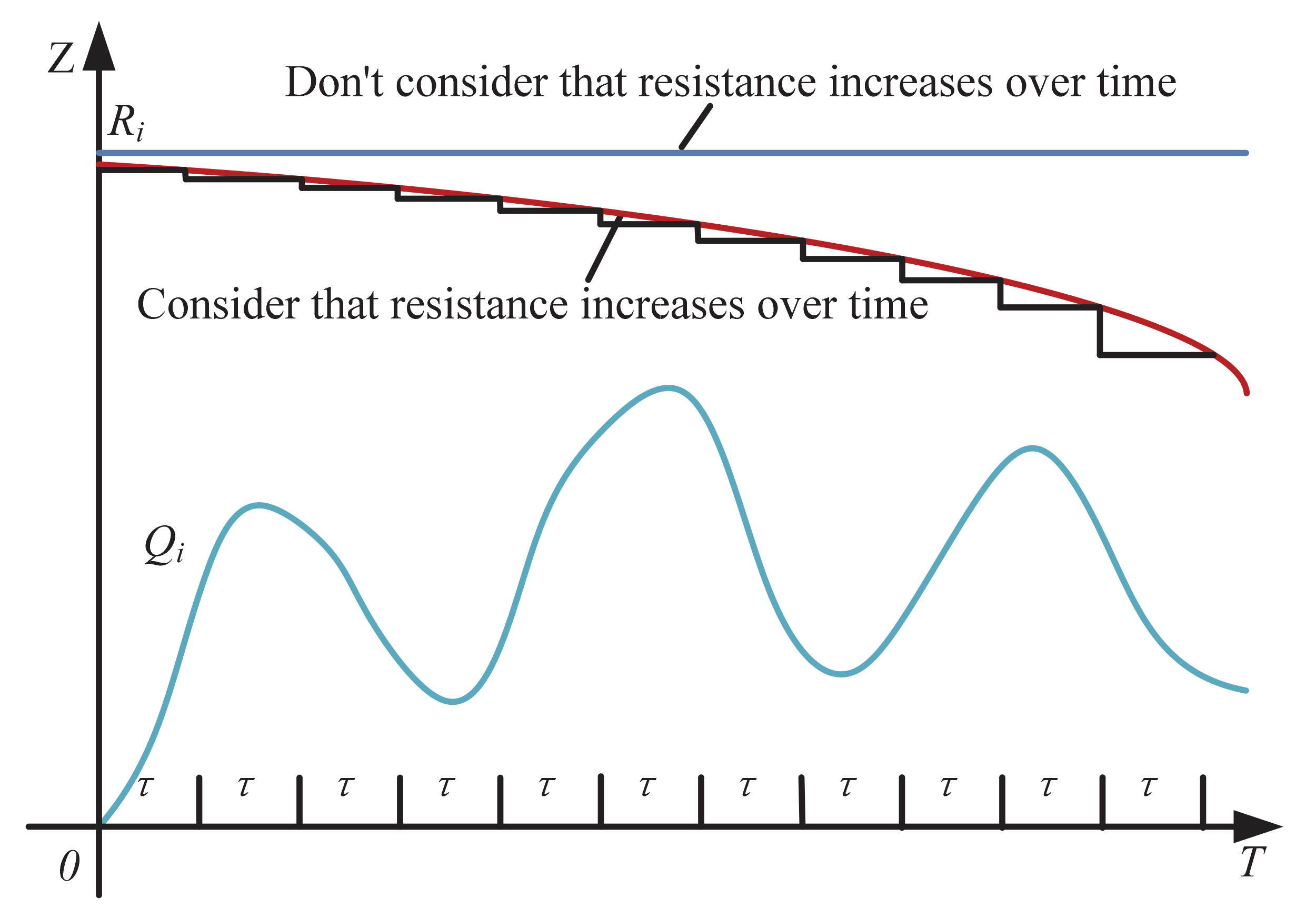
According to the definition of time-variant reliability [13,32,38], the design reference period T can be divided into m uniformly equal periods. Consequently, each period can be . The resistance stochastic process R(t) and dynamic load Q(t) can be discretized to obtain m random variables. It should be noted that the median value of the resistance in the i-th period equals the Ri value. Figure 1 illustrates distributions of resistance R(t) and variable load Q(t) over time.
The instantaneous value of the dynamic load Qi can be obtained statistically in the period. Generally, Qi can be regarded as an independent and identically distributed function. Based on the reliability theory of the series system, Equation (11) can be rewritten in the form below:
From the engineering point of view, is ’s s the maximum value. It should be indicated that Qi is independently and evenly distributed. Based on the principle of mechanism statistics, the probability distribution function of the maximum load effect in the reference period T can be formulated as:
In practical problems, the loading effect is usually approximated to the extreme value type I distribution with parameters and , subjected to the extreme value type I distribution with parameters and . This can be mathematically expressed in the form below:
Then probability distribution function and a new random variable Q’ with a probability density function and is defined. Accordingly, Equation (12) can be rewritten in the form below:
where denotes the joint probability density function of variables, and fA(a) is the probability density function of A. Meanwhile, denotes the probability distribution function of .
Equation (15) is a multi-dimensional integral problem, which requires a large amount of computation. In order to improve the computational efficiency, a new random variable is introduced
where stands for the following integral field:
is the inverse function of . Accordingly, the limit state function can be expressed as:
when the random variable Q′ is introduced, the general distribution form of Q′ is not specified. In other words, when Equation (18) is used as the limit state function to calculate the reliability index, the expression only contains the term. In this case, can be used as a variable so that the Q′ distribution is not required anymore in the whole analysis. However, in order to coordinate with the current unified design standard of structural reliability and make Q′ of engineering significance, Q′ is the maximum QT of Qi. Accordingly, Equation (18) can be rewritten as the following:
where is a random variable.
3.3. Double-Layer Nesting Optimization Method
There are both random and interval variables in Equation (19). At present, some methods have been proposed to solve this kind of problem. It is necessary to standardize the random variables.
In the analysis and calculation, the random variables need to be standardized. Equation (19) can be converted into:
where is the standard normal distribution function and U is the standard normal space variable.
By substituting Equation (20) into Equation (19), the limit state function in standard normal space can be obtained:
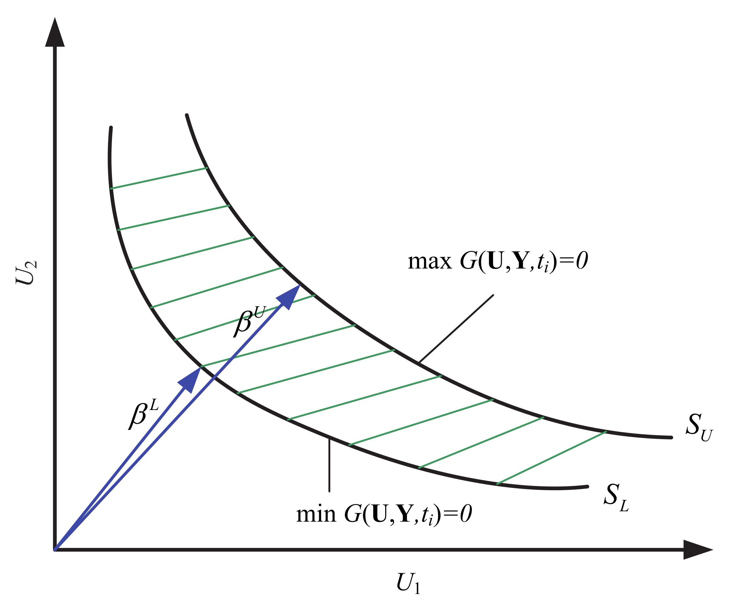
As the coexistence of random and interval variables, the limit state function (21) turns into a band in the parameter space as shown in Figure 2. The lower and upper boundaries are as follows:
where SL and SU represent the lower and upper boundaries, respectively.
The limit state region in Figure 2 shows failure probability Pf and reliability index β obtained from different Y-values of the limit state function on SL and SU planes. It should be indicated that both of these parameters are range values, in the form below:
Generally, the following two optimization problems are set to calculate the values of and -:
It should be reminded that time-variant failure probability falls in an interval. In most practical engineering problems, only the maximum failure probability is concerned. Consequently, only Equation (25) needs to be solved and the governing equations are reduced to the following expression:
Outer Optimization:
Inner layer optimization:
Equation (27) is a two-level nested optimization problem with complicated calculations and high computational expenses. Therefore, the optimization efficiency is difficult to meet the needs of engineering. Although decoupling strategies have been successfully applied to static hybrid reliability analysis problems, such as sequential single-loop strategies. It is a difficult problem to solve the time-variant reliability problem, because of time discretization, and inner and outer layer iteration. Also, a rigorous mathematical proof for decoupling strategy is lacking. Therefore, it is challenging to develop time-variant hybrid reliability decoupling strategies with good robustness and convergence.
4. A New Analysis Method of Structural Time-Variant Reliability with Random and Interval Variables
4.1. Establishment of Equivalent Model
In time-variant reliability analysis, uncertainty is divided into two kinds of uncertain variables, namely the random variable X and interval variable Y. In the present study, a novel method is initially presented. The random variable X is kept stable, while the interval variable Y obeys the uniform distribution. Therefore, it can be transformed into the following conventional time-variant reliability problem with only random variables:
where U and V denote the standard normal space, vectors transformed by X and Y, respectively. Moreover, is the limit state function of the transformation in the U-V space. For the equivalent model after transformation, the most probable point (MPP) in the standard normal space random variable (U + V) and its corresponding optimal value (,) can be calculated according to Equation (29).
4.2. Model Equivalence Proof
According to the studies of Breitung [39] on the asymptotic approximation of polynomial integrals, Madsen et al. [40] on first-order and second-order reliability analysis of series structures, and Madsen [41] on structural safety methods, it is seen that MPP has the highest probability density at all points on the limit state function. Therefore, (, ) is also the optimal solution to the following problem:
where fX,Y denotes the probability density function (PDF) of random variables X and Y.
Since all variables in the limit state function are independent of each other, Equation (30) can be modified as the following equation, based on the processing approach of the series system:
Since the random variable Y is uniformly distributed, the probability density function fY(Y) of the above-mentioned equation is a normal number. Therefore, Equation (31) can be rewritten into the following equation:
For the constrained optimization problem of Equation (32), Nocedal and Wright [42] proposed a numerical optimization approach according to the Karush-Kuhn-Tucker necessary conditions. Therefore, the optimal (, ) must meet the following equation:
where, λ1, λ2i, λ3i represent Lagrange multipliers.
Secondly, the reliability of the original mixed time-invariant model is investigated. As described above, in order to compute the maximum failure probability through the first-order second-moment approach, the MPP and the corresponding optimal value should be obtained. Moreover, the following optimization issues should be resolved:
Therefore, according to the properties of MPP, is the optimal solution of the following problem:
where Y is the interval variable. In the above mentioned equation, there is a sub-optimization problem , represented by an interval variable Y in the constraint, and the Karush–Kuhn–Tucker necessary condition is mathematically expressed as follows:
By substituting Equation (36) into Equation (35), the following optimization problem can be obtained:
Then, the Karush–Kuhn–Tucker necessary condition of Equation (37) is obtained, which is expressed the same as Equation (33). Therefore, it is mathematically proved that the original problem and the equivalent problem have the same solution when calculating reliability in this form. It should be indicated that the interval variable is treated with the uniform distribution, which is regarded as a random variable. in this situation, the limit state function of the time-variant reliability model with mixed uncertainties only contains random variable. Complex nested optimization problems for time variance can be successfully avoided.
4.3. Procedure
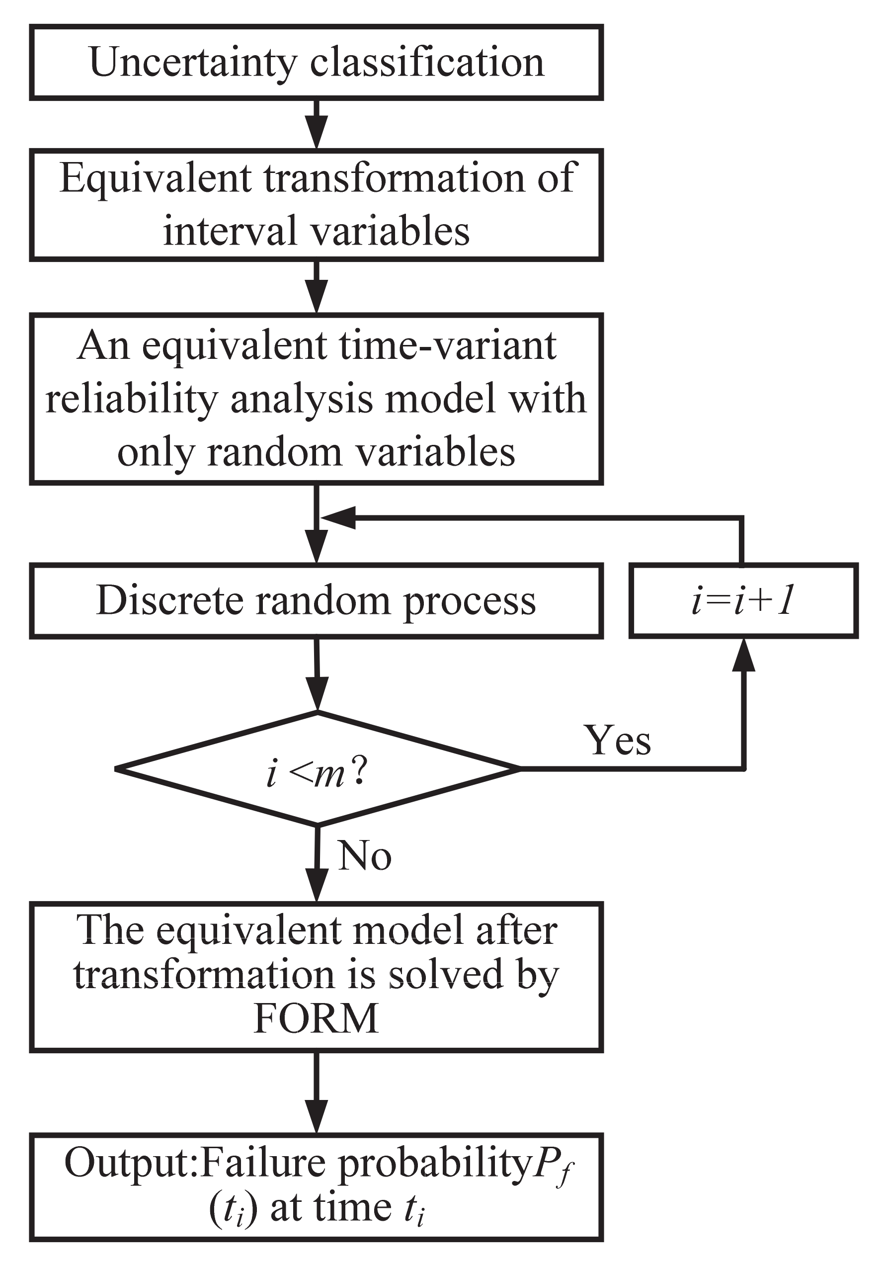
Based on the equivalent analysis above, the original structural time-variant reliability model of mixed variables is transformed into the equivalence model of the structural time-variant reliability model of mixed variables. As shown in the Figure 3, the specific steps are as follows:
- (1)
- The uncertainty in the structure is simply divided into two types according to the information given, including the probability random vector X and the non-probability vector Y (interval vector).
- (2)
- The interval variable Y is treated as a uniform distribution, which is regarded as a random variable.
- (3)
- The limit state function of the time-variant reliability model of the mixed uncertainties only contains the random variables X and Y. Then, the equivalent substitution model of the mixed reliability analysis is established.
- (4)
- The time parameters are discretized into m periods ti by the static transformation method. Meanwhile, the generalized resistance random process R(t) and the variable load Q(t) can be discretized. Therefore, the time-variant problem is changed into a time-invariant problem.
- (5)
- FORM is adopted to compute and solve the transformed equivalent mode in Equation (19). Then, an optimum can be obtained in each period.
- (6)
- The minimum reliability and the maximum failure probability of the model in each period is obtained.
5. Numerical Examples
In this section, the presented approach is applied to four examples, which include a mechanical part, a reinforced concrete short column of a structure, a roof truss structure, and a wing structure. In addition, the Monte Carlo Simulation approach (MCS) is employed to verify the feasibility of the presented method. The number of random numbers of each parameter generated by MCS in this study is ns = 1 × 10⁶.
5.1. Time-Variant Reliability Analysis of the Structure of a Mechanical Part
The change rule of the resistance of a mechanical part [10] with time is R(t) = R0exp(-at) MPa. Where a is the attenuation coefficient and interval variable, and R0 is the initial resistance, obeying the lognormal distribution of MPa. and are 336.3 MPa and 33.63 MPa, respectively. It is worth noting that the permanent load effect A follows the normal distribution of MPa. and are 66.25 MPa and 4.738 MPa. Taking τ = 1000 h as a period, the statistical value Qi of the dynamic load Q(t) in the ith period follows the extreme value I distribution. Parameters ατ and uτ equal ατ = 0.04493 MPa−1 and uτ = 49.77 MPa, respectively. Attenuation coefficient a I is interval variables. a I∈[1.9,2.1] × 10−5.
As can be seen from the Table 1, the reliability index when the sample number is 20,000, 50,000 and 100,000 is gradually close to the result when the sample number is 3,000,000. When the sample is 500,000, 1,000,000, 2,000,000 and 3,000,000, the calculation results in convergence. The sample number is 100,000, which can meet the accuracy requirement. However, in order to make the results more accurate and stable, this paper selected 1,000,000 times. With the increase of samples, the calculation time increases gradually. The calculation time is proportional to the number of samples. For example, when the number of samples is 3,000,000 and 1,000,000, the calculation time is 870.69 s and 300.82 s, respectively. The number of samples is three times larger, and the calculation time is nearly three times longer.
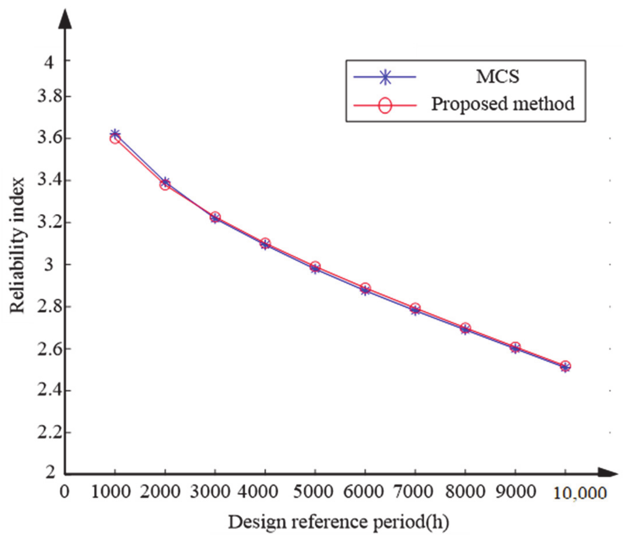
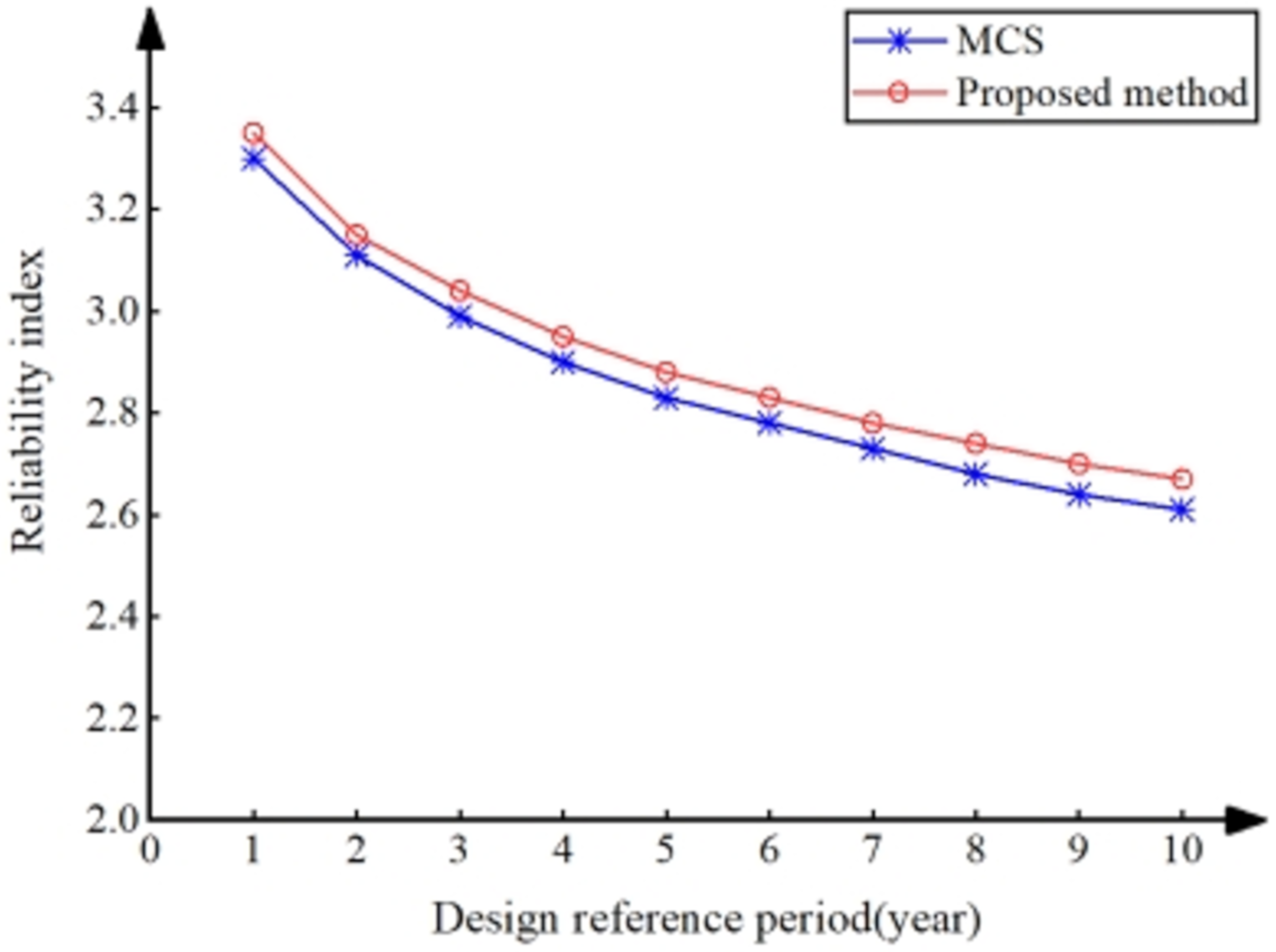
Figure 4 and Table 2 show the reliability index curve of a mechanical part in the design reference period. When the design reference period is 1000, 2000, 3000, 4000, 5000, 6000, 7000, 8000, 9000 and 10,000 respectively, the reliability indices are 3.600, 3.379, 3.227, 3.102, 2.991, 2.889, 2.793, 2.699, 2.608 and 2.518 respectively. Therefore, it is observed that as the design base period extends, the reliability of this part decreases gradually. Correspondingly, the failure probability will gradually increase, which is consistent with the actual situation.
MCS is a more accurate method to solve structural reliability problems, which is generally adopted as an accurate result to verify the accuracy of other methods. In Table 2, when t = 1000, the maximum error is 0.62%, and when t = 4000, the minimum error is 0.27%, which is within the engineering allowable range. The results of the proposed method are very close to those of MCS method, which indicates that the proposed method is effective and feasible. In this study, the limit state function only needs to be called 72 times, while it needs to be called 9,984,164 times through MCS method. The running time of the MCS method is 300.82 s, while the running time of the current method is 0.089s. The total number of calls to limit state functions in this method is many orders of magnitude less than that in the MCS method.
5.2. A Short Column of the Reinforced Concrete of a Structure
The example discussed in this section is modified according to the literature [43]. The width and height of the cross-section of the reinforced concrete short column of a structure are denoted as B and h, respectively. Moreover, the parameter values of the width and height of the cross-section are interval values, whose parameter values are [270 mm, 330 mm] and [315 mm, 380 mm], respectively.
The strength grade of the concrete is C30 and the area of the steel bar in the column is 1811.28mm2, which is a grade II steel bar. Moreover, R(t), G and Q denote the random resistance process of the reinforced concrete short column, the permanent load effect and the variable load effect, respectively. Table 3 presents the specific parameters and distribution.
R(t) is mathematically defined as:
where fc and fy denote the compressive strength of the concrete and the yield strength of reinforcement, respectively.
The resistance variation coefficients and are:
The limit state function is mathematically expressed as:
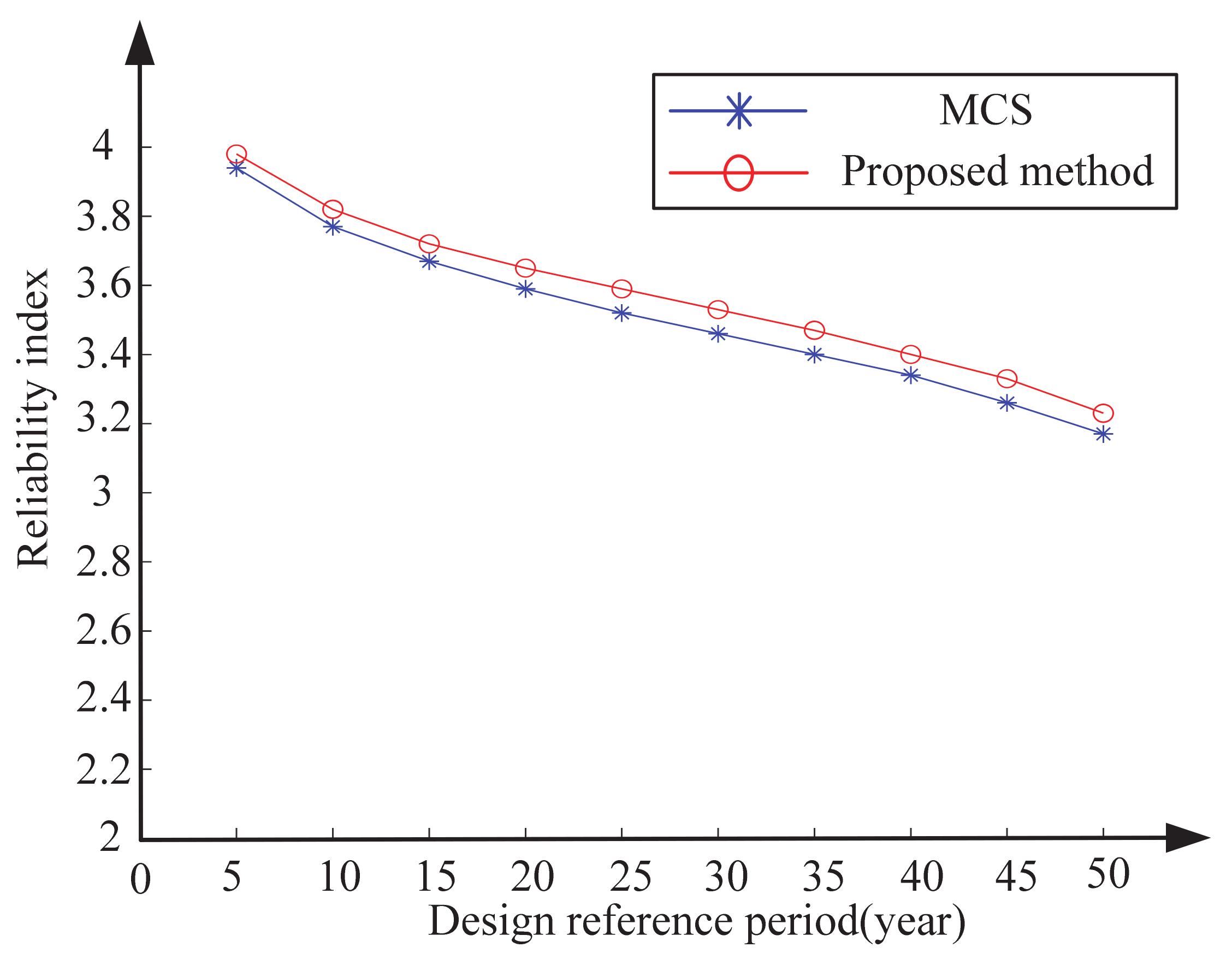
From Table 4, it is proved once again that the results of MCS method are convergent. With the increase of the number of samples, the calculation time increases linearly. Figure 5 illustrates that as the design reference period exceeds, the reliability of the structure or product gradually decreases. As can be seen from Table 5, the errors of the current method and MCS method are as follows: 1.02%, 1.33%, 1.36%, 1.67%, 1.99%, 2.02%, 2.06%, 1.80%, 2.15% and 1.89%. The maximum error is 2.02 and the minimum error is 1.02. The error can meet the needs of engineering, moreover the accuracy of the present method is proved again. From viewpoint of computational efficiency, the total number of calls to limit state functions in this method is only 171, while it is 9,997,832 times for the MCS method. The MCS method runs in 673.8 s, and the current method runs in 0.12 s. Therefore, it is proved that the computational efficiency of the presented approach is much higher than that of the MCS method. The results of an example show that the proposed method is an effective approach.
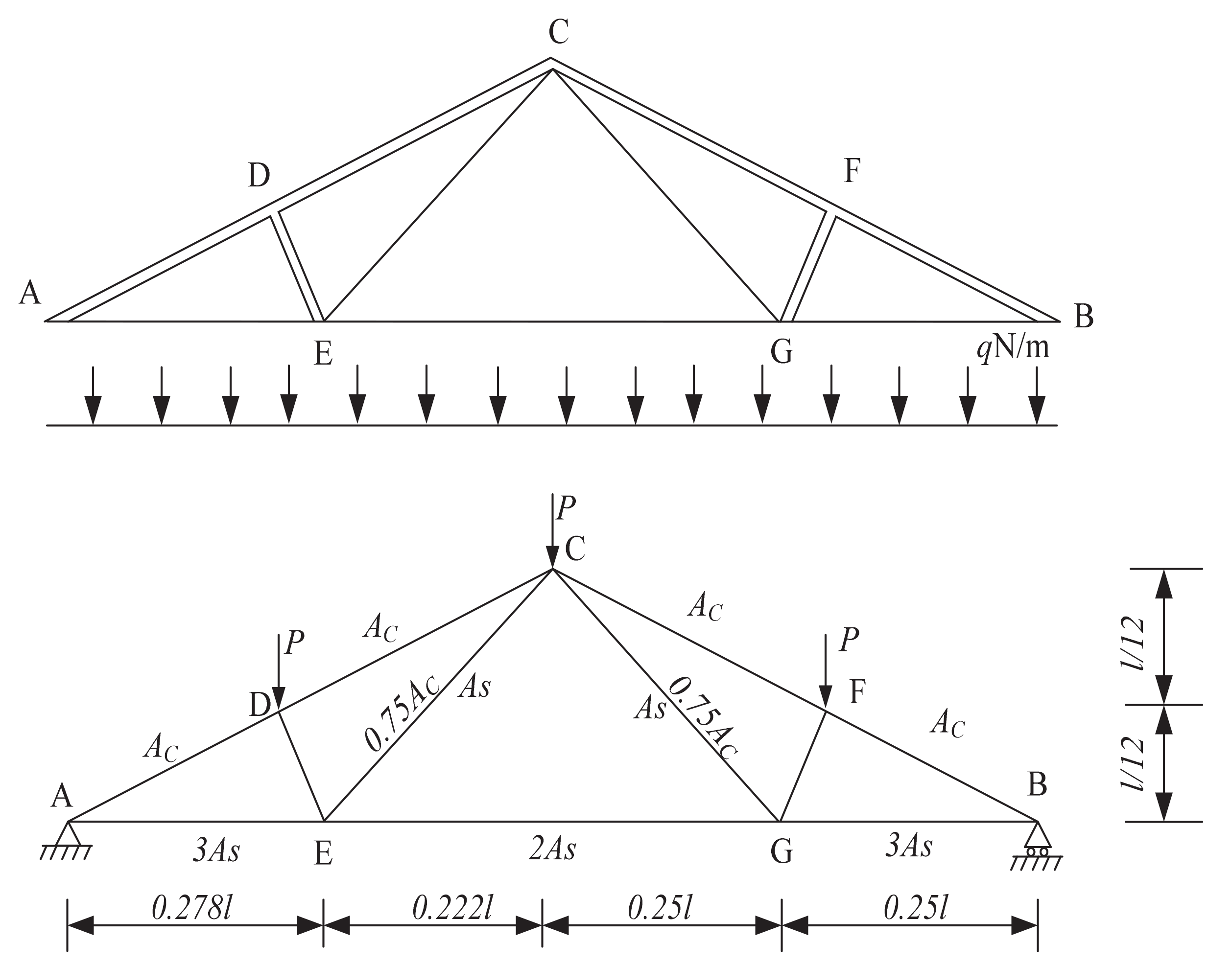
5.3. A Roof Truss Structure
Figure 6 shows that the bottom and tension members are made of steel, and the top and pressure members are reinforced with concrete [44,45].
The roof is subjected to evenly distributed load q(t), where q(t) can be converted to the equivalent nodal force P = q(t)l/4. Moreover, the vertical displacement at node C can be expressed as follows:
where AC and AS denote the cross-sectional areas of the cement and steel rods, respectively. It should be indicated that AC and AS are interval variables with the ranges of [0.0323 m2, 0.0357 m2] and [8.93 × 10⁻⁴ m2, 9.87 × 10⁻⁴ m2], respectively. Moreover, EC and ES denote their elastic modulus, respectively. During the loading process, the vertical displacement of node C should be less than D(t) that decays with time. The decay rule is: D(t)=D0[1 + ln(1 – 0.0002t)], and D0 is the initial displacement. Table 6 lists the specific situation of the random variable in this problem. The design base period is assumed to be T = 10 years. The limit state function is defined as:
It can be seen again from Table 7 that the calculation results based on MCS method are convergent, and the calculation time increases linearly with the increase of the number of samples. As shown in Figure 7 and Table 8, the reliability indices are 3.35, 3.15, 3.04, 2.95, 2.88, 2.83, 2.78, 2.74, 2.70 and 2.67, which decreases significantly with time. Table 7 presents that the maximum error between the results obtained by this method. It can be seen that the errors are 1.52%, 1.29%, 1.67%, 1.72%, 1.77%, 1.80%, 1.83%, 2.24%, 2.27% and 2.30%, respectively. Compared with MCS method, the maximum error is 2.30%. Once again, it should be indicated that the results obtained by this method are very accurate. From the viewpoint of computational efficiency, this method only calls the limit state function 511 times, while MCS method calls the limit state function 9,999,463 times. The running time of MCS method is 384.4 seconds, while the running time of the current method is 0.115 s. This shows the effectiveness of the presented method.
5.4. A Wing Structure
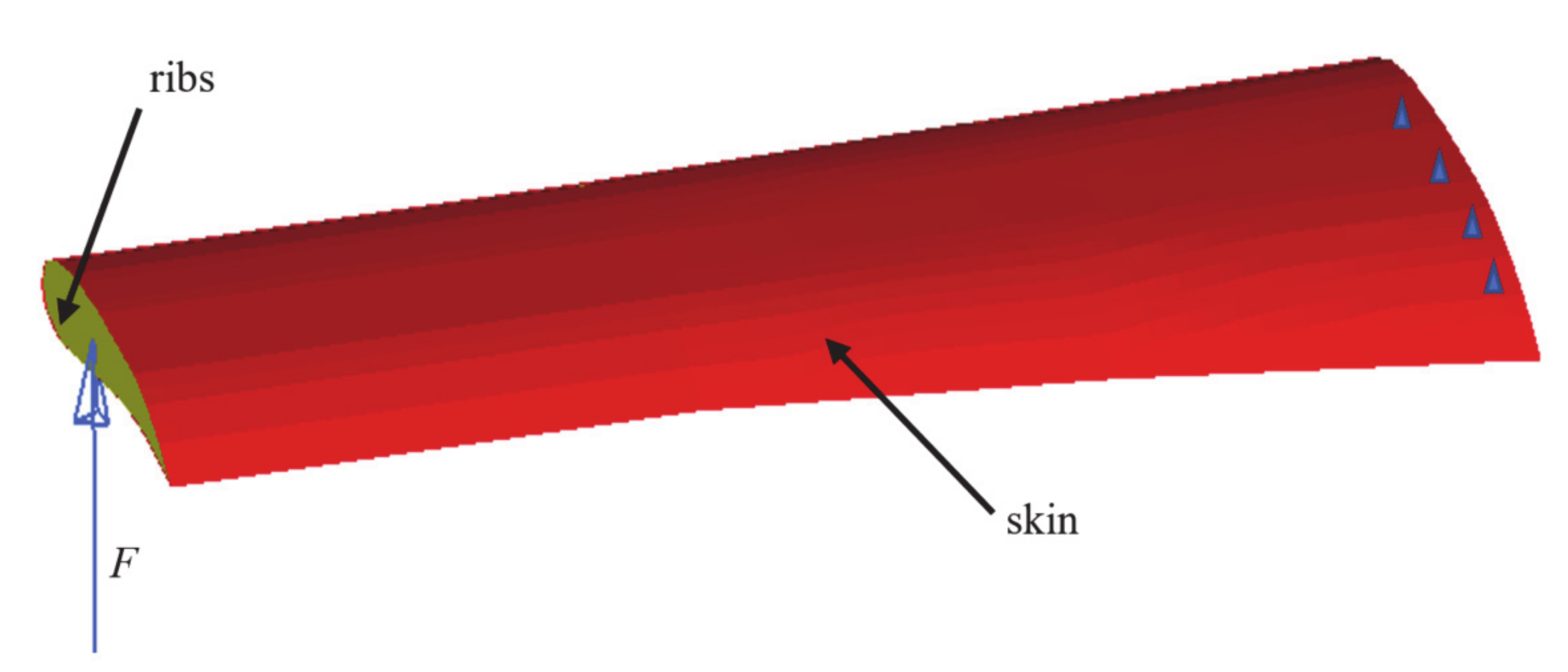
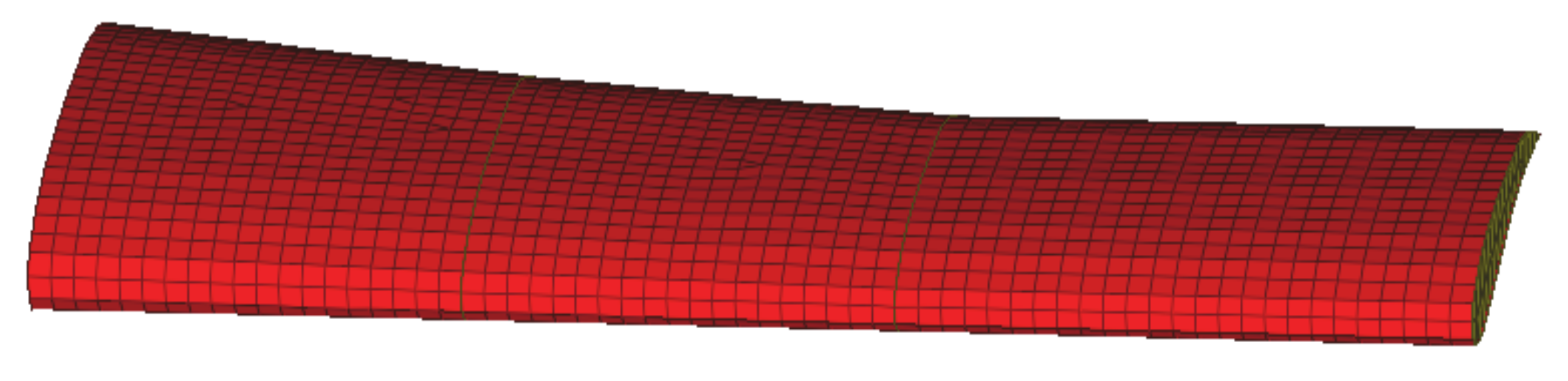
The reliability problem of the wing structure [45] is adopted to verify the application of the presented approach in actual engineering. Figure 8 shows that the wing structure consists of three ribs and a skin. The load F is applied to the left side of the wing, and the other side is constrained in three directions.
The young’s modulus of the rib as an interval variable, the Poisson’s ratio and the density, are E1, 0.35 and 4.0 × 10³ kg/m3, respectively. Moreover, the young’s modulus of the skin as an interval variable, the Poisson’s ratio and the density are E2, 0.35 and 1.8 × 10³ kg/m3, respectively. It is worth noting that the rib thickness and skin thickness are recorded as th and s, respectively.
The variables {th, s, E1, E2}T are independent from each other: th~N(3.0, 0.022), s~N(3.0, 0.022) E1∈[42,750 MPa, 4,7250 MPa] E2∈[28,500 MPa, 31,500 MPa]. The wing structure requires that during the design baseline period T = 10 years, the vertical deformation D(t) of the wing surface during the loading process should not exceed D(t) = D0[1 + ln(1 − 0.0002t)], and D0 is the initial displacement. D0~N(85, 7.52).When the design life is 5 years, the time-variant load is the F, and the maximum variable load is subjected to an extreme value I distribution, , . Therefore, the limit state function of the wing structure can be defined as:
where Dmax() denotes the maximum displacement of the structure, which can be achieved through the finite element method (FEM).
Figure 9 shows that the wing structure adopts the finite element model composed of hexahedron elements and four-node shell elements. The model has 2899 elements and 2869 nodes, respectively. Opstruct software is used to calculate this finite element model. Then, the second-order response surface model is constructed through the Latin square experimental design, which is mathematically expressed as follows:
Five sampling points are randomly chosen in the design space to verify the accuracy of the approximate model. As shown in Table 9, the relative errors between the response surface results based on these points and the simulation model results are 0.0077%, 0.0026%, 0.0162%, 0.0214% and 0.0035%. The maximum error is much less than 0.1%, and the response surface approximation model has high accuracy, which is completely acceptable in engineering.
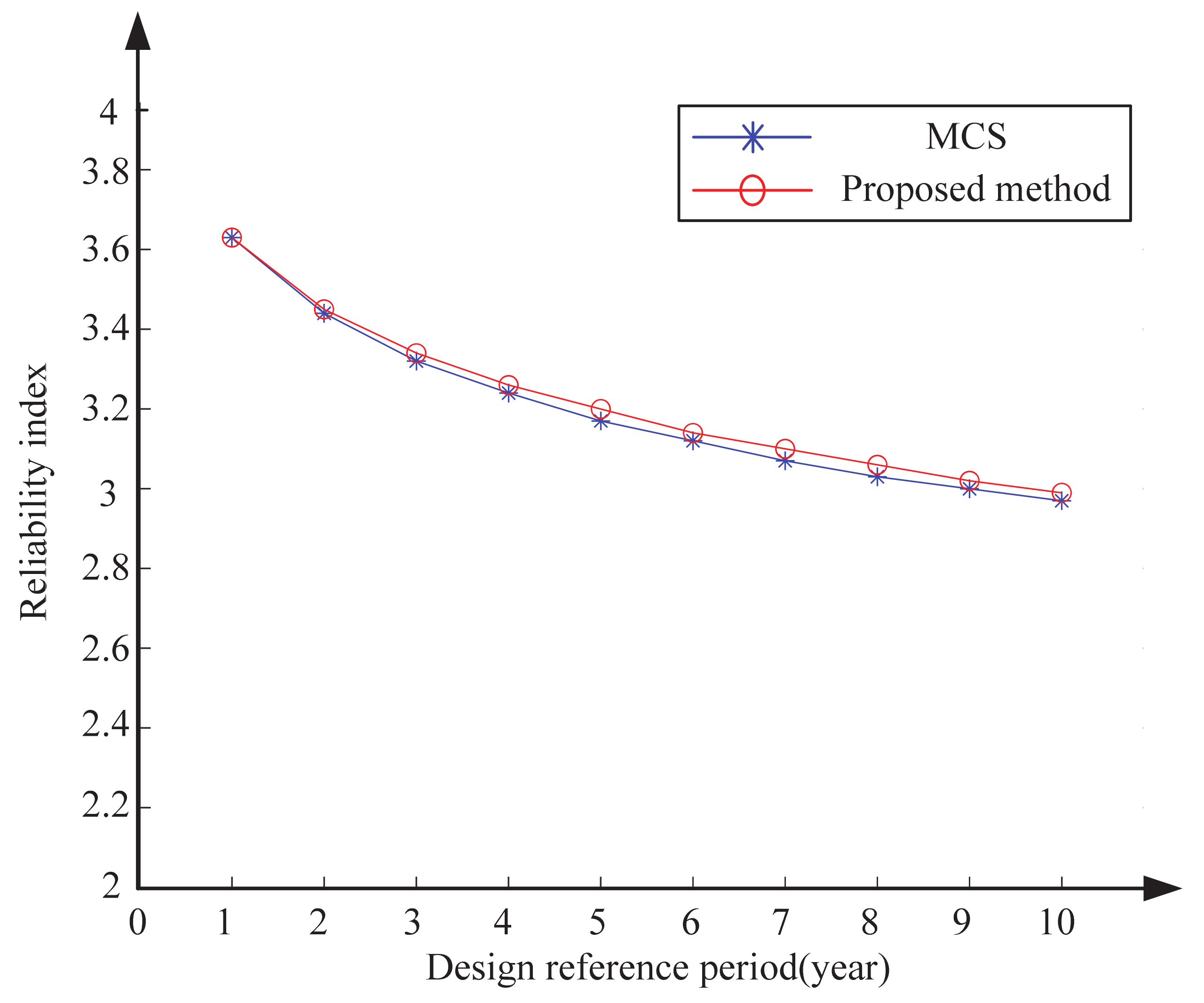
Figure 10 and Table 10 present reliability indices under the design reference period for a certain wing surface structure. The reliability indexes calculated by the current method are 3.63, 3.45, 3.34, 3.26, 3.20, 3.14, 3.10, 3.06, 3.02 and 2.99. The calculation results show that due to the attenuation of dynamic load and maximum displacement, the reliability index is no longer a fixed value, but gradually decreases from 3.63 to 2.99 with the design lifetimes increase. Comparing the obtained results with calculations through the MCS demonstrates that the maximum error between the two methods is 0.91%, indicating the high accuracy of the presented approach. In terms of computational efficiency, the total number of calls to the response surface approximation model of limit state function is only 83, while MCS needs to call 9,991,818.
6. Conclusions
In the present article, a time-variant reliability analysis method is proposed for mixed-variable structures. The time-variant reliability problem of structures with mixed variables is transformed into a time-variant reliability problem of structures with random variables. Then the stochastic process is discretized and the static limit state functions of different periods are obtained. After the original problem is changed into an invariant reliability problem, the first-order second-moment method is applied to solve the problem. Finally, the reliability index under the design base period is obtained.
In order to evaluate the performance of the presented approach, it is applied to three numerical and one engineering case studies. Obtained results show that in the studied cases, the performance of the presented approach is very close to that of the Monte Carlo method. Moreover, it is found that the proposed algorithm avoids multi-layer nesting optimization and greatly improves computational efficiency.
The present method can be extended to time-variant reliability analysis problems with convex set variables and probability variables, and to multidisciplinary reliability analysis problems. When the range of interval parameters are big, the computational expenses of the proposed method cannot be justified. In order to resolve this shortcoming, improving the efficiency of time-variant hybrid reliability analyses will be discussed in the near future.
Author Contributions
Conceptualization, F.L.; methodology, F.L.; validation, J.R. and H.Z.; formal analysis, Y.Y.; investigation, Y.Y; data curation, H.Z.; writing—review and editing, J.R. and H.Z. All authors have read and agreed to the published version of the manuscript.
Funding
This work was partially supported by the Science and Technology Program of Guangzhou (202102010428), National Natural Science Foundation of China (11772070,11672104,11902085), Hunan Provincial Natural Science Foundation of China (2019JJ40296) and the Open Fund of Key Laboratory of Bridge Engineering Safety Control by Department of Education (19KB06).
Data Availability Statement
Not applicable.
Conflicts of Interest
The authors declare no conflict of interest.
References
- Zhang, D.; Zhang, N.; Ye, N.; Fang, J.; Han, X. Hybrid learning algorithm of radial basis function networks for reliability analysis. IEEE Trans. Reliab. 2020, 1–14. [Google Scholar] [CrossRef]
- Wu, J.; Zhang, D.; Jiang, C.; Han, X.; Li, Q. On reliability analysis method through rotational sparse grid nodes. Mech. Syst. Signal Process. 2021, 147, 107106. [Google Scholar] [CrossRef]
- Liu, J.; Wen, G.; Xie, Y.M. Layout optimization of continuum structures considering the probabilistic and fuzzy directional uncertainty of applied loads based on the cloud model. Struct. Multidiscip. Optim. 2016, 53, 81–100. [Google Scholar] [CrossRef]
- Wang, H.; Liu, J.; Wen, G. An efficient evolutionary structural optimization method for multi-resolution designs. Struct. Multidiscip. Optim. 2020, 62, 787–803. [Google Scholar] [CrossRef]
- Huang, Z.L.; Zhang, J.W.; Kumar, T.; Yang, T.G.; Deng, S.G.; Li, F.Y. Robust Optimization for micromachine design problems involving multimodal distributions. IEEE Access 2019, 7, 91838–91849. [Google Scholar] [CrossRef]
- Hasofer, A.M.; Lind, N.C. Exact and invariant second-moment code format. J. Eng. Mech. Div. 1974, 100, 111–121. [Google Scholar] [CrossRef]
- Rackwitz, R.; Flessler, B. Structural reliability under combined random load sequences. Comput. Struct. 1978, 9, 489–494. [Google Scholar] [CrossRef]
- Breitung, K.; Hohenbichler, M. Asymptotic approximations for multivariate integrals with an application to multinormal probabilities. J. Multivar. Anal. 1989, 30, 80–97. [Google Scholar] [CrossRef] [Green Version]
- Bennett, R.M. Structural analysis methods for system reliability. Struct. Saf. 1990, 7, 109–114. [Google Scholar] [CrossRef]
- Jiang, C.; Huang, X.P.; Han, X.; Zhang, D.Q. A Time-variant reliability analysis method based on stochastic process discretization. J. Mech. Des. 2014, 136. [Google Scholar] [CrossRef]
- Wang, L.; Ma, Y.; Yang, Y.; Wang, X. Structural design optimization based on hybrid time-variant reliability measure under non-probabilistic convex uncertainties. Appl. Math. Model. 2019, 69, 330–354. [Google Scholar] [CrossRef]
- Du, X. Time-dependent mechanism reliability analysis with envelope functions and first-order approximation. J. Mech. Des. 2014, 136, 081010. [Google Scholar] [CrossRef]
- Li, F.; Liu, J.; Yan, Y.; Rong, J.; Yi, J.; Wen, G. A time-variant reliability analysis method for non-linear limit-state functions with the mixture of random and interval variables. Eng. Struct. 2020, 213, 110588. [Google Scholar] [CrossRef]
- Rice, S.O. Mathematical analysis of random noise. Bell Syst. Tech. J. 1944, 23, 282–332. [Google Scholar] [CrossRef]
- Andrieu-Renaud, C.; Sudret, B.; Lemaire, M. The PHI2 method: A way to compute time-variant reliability. Reliab. Eng. Syst. Saf. 2004, 84, 75–86. [Google Scholar] [CrossRef]
- Sudret, B. Analytical derivation of the outcrossing rate in time-variant reliability problems. Struct. Infrastruct. Eng. 2008, 4, 353–362. [Google Scholar] [CrossRef]
- Mori, Y.; Ellingwood, B.R. Time-dependent system reliability analysis by adaptive importance sampling. Struct. Saf. 1993, 12, 59–73. [Google Scholar] [CrossRef]
- Singh, A.; Mourelatos, Z.P.; Nikolaidis, E. An importance sampling approach for time-dependent reliability. Proc. Pap. 2011, 1077–1088. [Google Scholar] [CrossRef]
- Au, S.K.; Beck, J.L. Estimation of small failure probabilities in high dimensions by subset simulation. Probabilistic Eng. Mech. 2001, 16, 263–277. [Google Scholar] [CrossRef] [Green Version]
- Wang, Z.; Mourelatos, Z.P.; Li, J.; Baseski, I.; Singh, A. Time-dependent reliability of dynamic systems using subset simulation with splitting over a series of correlated time intervals. J. Mech. Des. 2014, 136. [Google Scholar] [CrossRef] [Green Version]
- Sonal, S.D.; Ammanagi, S.; Kanjilal, O.; Manohar, C.S. Experimental estimation of time variant system reliability of vibrating structures based on subset simulation with Markov chain splitting. Reliab. Eng. Syst. Saf. 2018, 178, 55–68. [Google Scholar] [CrossRef]
- Chen, J.-B.; Li, J. The extreme value distribution and dynamic reliability analysis of nonlinear structures with uncertain parameters. Struct. Saf. 2007, 29, 77–93. [Google Scholar] [CrossRef]
- Hu, Z.; Du, X. A sampling approach to extreme value distribution for time-dependent reliability analysis. J. Mech. Des. 2013, 135. [Google Scholar] [CrossRef]
- Papadopoulos, V.; Giovanis, D.G.; Lagaros, N.D.; Papadrakakis, M. Accelerated subset simulation with neural networks for reliability analysis. Comput. Methods Appl. Mech. Eng. 2012, 223–224, 70–80. [Google Scholar] [CrossRef]
- Wang, Z.; Wang, P. A Nested extreme response surface approach for time-dependent reliability-based design optimization. J. Mech. Des. 2012, 134. [Google Scholar] [CrossRef]
- Wang, Z.; Wang, P. A new approach for reliability analysis with time-variant performance characteristics. Reliab. Eng. Syst. Saf. 2013, 115, 70–81. [Google Scholar] [CrossRef]
- Jones, D.R.; Schonlau, M.; Welch, W.J. Efficient Global optimization of expensive black-box functions. J. Glob. Optim. 1998, 13, 455–492. [Google Scholar] [CrossRef]
- Zhang, D.; Han, X.; Jiang, C.; Liu, J.; Li, Q. Time-dependent reliability analysis through response surface method. J. Mech. Des. 2017, 139. [Google Scholar] [CrossRef]
- Li, C.C.; Der Kiureghian, A. Optimal discretization of random fields. J. Eng. Mech. Asce 1993, 119, 1136–1154. [Google Scholar] [CrossRef]
- Cazuguel, M.; Renaud, C.; Cognard, J.Y. Time-variant reliability of nonlinear structures: Application to a representative part of a plate floor. Qual. Reliab. Eng. Int. 2006, 22, 101–118. [Google Scholar] [CrossRef]
- Gong, C.; Frangopol, D.M. An efficient time-dependent reliability method. Struct. Saf. 2019, 81, 101864. [Google Scholar] [CrossRef]
- Jiang, C.; Huang, X.P.; Wei, X.P.; Liu, N.Y. A time-variant reliability analysis method for structural systems based on stochastic process discretization. Int. J. Mech. Mater. Des. 2017, 13, 173–193. [Google Scholar] [CrossRef]
- Jiang, C.; Wei, X.P.; Wu, B.; Huang, Z.L. An improved TRPD method for time-variant reliability analysis. Struct. Multidiscip. Optim. 2018, 58, 1935–1946. [Google Scholar] [CrossRef]
- Ben-Haim, Y. A non-probabilistic concept of reliability. Struct. Saf. 1994, 14, 227–245. [Google Scholar] [CrossRef]
- Du, X.; Sudjianto, A. Reliability-Based Design with the Mixture of Random and Interval Variables. In Proceedings of the ASME 2003 International Design Engineering Technical Conferences and Computers and Information in Engineering Conference, Online, Virtual, 17–19 August 2021; pp. 55–62. [Google Scholar]
- Das Neves Carneiro, G.; António, C.C. Robustness and reliability of composite structures: Effects of different sources of uncertainty. Int. J. Mech. Mater. Des. 2019, 15, 93–107. [Google Scholar] [CrossRef]
- Huang, Z.L.; Jiang, C.; Li, X.M.; Wei, X.P.; Fang, T.; Han, X. A single-loop approach for time-variant reliability-based design optimization. IEEE Trans. Reliab. 2017, 66, 651–661. [Google Scholar] [CrossRef]
- Jiang, C.; Wei, X.; Huang, Z.; Liu, J. An outcrossing rate model and its efficient calculation for time-dependent system reliability analysis. J. Mech. Des. 2017, 139, 041402. [Google Scholar] [CrossRef]
- Breitung, K. Asymptotic approximations for probability integrals. Probabilistic Eng. Mech. 1989, 4, 187–190. [Google Scholar] [CrossRef]
- Madsen, H.O.; Krenk, S.; Lind, N.C. Method of Structural Safety; Courier Corporation: Tokyo, Japan, 2006. [Google Scholar]
- Madsen, H.O. First order vs. second order reliability analysis of series structures. Struct. Saf. 1985, 2, 207–214. [Google Scholar] [CrossRef]
- Nocedal, J.; Wright, S.J. Numerical Optimization, 2nd ed.; Springer: Berlin/Heidelberg, Germany, 2006. [Google Scholar]
- Gong, J.-X.; Yi, P. A robust iterative algorithm for structural reliability analysis. Struct. Multidiscip. Optim. 2011, 43, 519–527. [Google Scholar] [CrossRef]
- Wei, P.; Lu, Z.; Hao, W.; Feng, J.; Wang, B. Efficient sampling methods for global reliability sensitivity analysis. Comput. Phys. Commun. 2012, 183, 1728–1743. [Google Scholar] [CrossRef]
- Yang, X.; Liu, Y.; Gao, Y.; Zhang, Y.; Gao, Z. An active learning kriging model for hybrid reliability analysis with both random and interval variables. Struct. Multidiscip. Optim. 2015, 51, 1003–1016. [Google Scholar] [CrossRef]
Figure 1.
Distribution of resistance R(t) and variable load Q(t) over time.

Figure 2.
Limit state region.

Figure 3.
Algorithm flow chart.

Figure 4.
The reliability index curve of a mechanical part in the design reference period.

Figure 5.
Reliability index curves of reinforced concrete short column of a structure in design reference period.
Figure 5.
Reliability index curves of reinforced concrete short column of a structure in design reference period.

Figure 6.
Roof truss model.

Figure 7.
Reliability index curve of roof structure in design reference period.

Figure 8.
A wing structure.

Figure 9.
Finite element model of the wing structure.

Figure 10.
Reliability index curve of machine wing surface structure in design reference period.


Table 1.
Calculation results of Monte Carlo method under different sample numbers.
| ns | Design Reference Period (h) | Time (s) | |||||||||
|---|---|---|---|---|---|---|---|---|---|---|---|
| 1000 | 2000 | 3000 | 4000 | 5000 | 6000 | 7000 | 8000 | 9000 | 10,000 | ||
| 20,000 | 3.481 | 3.390 | 3.156 | 2.989 | 2.903 | 2.776 | 2.669 | 2.628 | 2.530 | 2.457 | 5.26 |
| 50,000 | 3.673 | 3.470 | 3.279 | 3.179 | 3.062 | 2.921 | 2.802 | 2.708 | 2.624 | 2.556 | 15.78 |
| 100,000 | 3.719 | 3.414 | 3.291 | 3.102 | 2.970 | 2.870 | 2.794 | 2.694 | 2.604 | 2.519 | 30.37 |
| 500,000 | 3.580 | 3.350 | 3.211 | 3.104 | 2.999 | 2.901 | 2.793 | 2.697 | 2.603 | 2.515 | 149.68 |
| 1,000,000 | 3.622 | 3.393 | 3.219 | 3.094 | 2.979 | 2.876 | 2.781 | 2.690 | 2.600 | 2.510 | 300.82 |
| 2,000,000 | 3.612 | 3.388 | 3.223 | 3.099 | 2.984 | 2.877 | 2.782 | 2.688 | 2.597 | 2.508 | 561.31 |
| 3,000,000 | 3.599 | 3.370 | 3.215 | 3.094 | 2.981 | 2.880 | 2.786 | 2.692 | 2.597 | 2.509 | 870.69 |
Table 2.
Reliability index of the mechanical part in each design reference period.
| Methods | Design Reference Period (h) | |||||||||
|---|---|---|---|---|---|---|---|---|---|---|
| 1000 | 2000 | 3000 | 4000 | 5000 | 6000 | 7000 | 8000 | 9000 | 10,000 | |
| MCS | 3.622 | 3.393 | 3.219 | 3.094 | 2.979 | 2.876 | 2.781 | 2.690 | 2.600 | 2.510 |
| Proposed method | 3.600 | 3.379 | 3.227 | 3.102 | 2.991 | 2.889 | 2.793 | 2.699 | 2.608 | 2.518 |
| Deviation/% | 0.62 | 0.41 | 0.25 | 0.27 | 0.40 | 0.45 | 0.43 | 0.34 | 0.31 | 0.32 |
Table 3.
Variable distribution of reinforced concrete short columns of a structure.
| Parameter | Mean μ | Standard Deviation σ | Type of Distribution |
|---|---|---|---|
| G(kN) | 530 | 37.1 | normal |
| QT(kN) | 700 | 203 | Extreme I type |
| fc(N/mm2) | 26.1 | 4.437 | normal |
| fy(N/mm2) | 384 | 28.591 | normal |
Table 4.
Calculation results of Monte Carlo method under different sample numbers.
| ns | Design Reference Period (Year) | Time (s) | |||||||||
|---|---|---|---|---|---|---|---|---|---|---|---|
| 5 | 10 | 15 | 20 | 25 | 30 | 35 | 40 | 45 | 50 | ||
| 30,000 | 3.72 | 3.59 | 3.54 | 3.40 | 3.38 | 3.35 | 3.31 | 3.29 | 3.23 | 3.18 | 8.5 |
| 100,000 | 4.10 | 3.81 | 3.69 | 3.61 | 3.54 | 3.49 | 3.43 | 3.37 | 3.32 | 3.22 | 32.4 |
| 500,000 | 3.94 | 3.78 | 3.68 | 3.58 | 3.50 | 3.46 | 3.40 | 3.34 | 3.27 | 3.18 | 157.4 |
| 1,000,000 | 3.94 | 3.77 | 3.67 | 3.59 | 3.52 | 3.46 | 3.40 | 3.34 | 3.26 | 3.17 | 673.8 |
| 2,000,000 | 3.94 | 3.78 | 3.68 | 3.60 | 3.53 | 3.47 | 3.41 | 3.35 | 3.27 | 3.17 | 734.8 |
| 3,000,000 | 3.94 | 3.77 | 3.66 | 3.58 | 3.52 | 3.46 | 3.39 | 3.34 | 3.26 | 3.16 | 1153.8 |
Table 5.
Reliability index of each design reference period of the short column.
| Methods | Design Reference Period (Year) | |||||||||
|---|---|---|---|---|---|---|---|---|---|---|
| 5 | 10 | 15 | 20 | 25 | 30 | 35 | 40 | 45 | 50 | |
| MCS | 3.94 | 3.77 | 3.67 | 3.59 | 3.52 | 3.46 | 3.40 | 3.34 | 3.26 | 3.17 |
| Proposed method | 3.98 | 3.82 | 3.72 | 3.65 | 3.59 | 3.53 | 3.47 | 3.40 | 3.33 | 3.23 |
| Deviation/% | 1.02 | 1.33 | 1.36 | 1.67 | 1.99 | 2.02 | 2.06 | 1.80 | 2.15 | 1.89 |
Table 6.
Distribution of random variables of the roof truss structure.
| Parameter | Mean μ | Standard Deviation σ | Type of Distribution |
|---|---|---|---|
| q(N/m) | 20,000 | 1600 | Extreme I type |
| D0(m) | 0.022 | 0.001 | normal |
| l(m) | 12 | 0.24 | normal |
| ES(N/m2) | 2×10¹¹ | 1.4×10¹⁰ | normal |
| EC(N/m2) | 3×10¹⁰ | 2.4×10⁹ | normal |
Table 7.
Calculation results of Monte Carlo method under different sample numbers.
| ns | Design Reference Period (Year) | Time (s) | |||||||||
|---|---|---|---|---|---|---|---|---|---|---|---|
| 1 | 2 | 3 | 4 | 5 | 6 | 7 | 8 | 9 | 10 | ||
| 30,000 | 3.41 | 3.20 | 3.10 | 2.94 | 2.88 | 2.82 | 2.76 | 2.72 | 2.68 | 2.66 | 9.9 |
| 100,000 | 3.34 | 3.15 | 3.04 | 2.94 | 2.85 | 2.78 | 2.73 | 2.69 | 2.65 | 2.62 | 38.4 |
| 500,000 | 3.33 | 3.13 | 3.02 | 2.92 | 2.83 | 2.78 | 2.73 | 2.68 | 2.65 | 2.62 | 205.5 |
| 1,000,000 | 3.30 | 3.11 | 2.99 | 2.90 | 2.83 | 2.78 | 2.73 | 2.68 | 2.64 | 2.61 | 384.4 |
| 2,000,000 | 3.31 | 3.11 | 2.99 | 2.91 | 2.83 | 2.78 | 2.73 | 2.68 | 2.64 | 2.61 | 763.8 |
| 3,000,000 | 3.31 | 3.11 | 2.99 | 2.90 | 2.83 | 2.77 | 2.72 | 2.68 | 2.64 | 2.61 | 1153.8 |
Table 8.
Reliability index of the roof truss structure in each design reference period.
| Methods | Design Reference Period (Year) | |||||||||
|---|---|---|---|---|---|---|---|---|---|---|
| 1 | 2 | 3 | 4 | 5 | 6 | 7 | 8 | 9 | 10 | |
| MCS | 3.30 | 3.11 | 2.99 | 2.90 | 2.83 | 2.78 | 2.73 | 2.68 | 2.64 | 2.61 |
| Proposed method | 3.35 | 3.15 | 3.04 | 2.95 | 2.88 | 2.83 | 2.78 | 2.74 | 2.70 | 2.67 |
| Deviation/% | 1.52 | 1.29 | 1.67 | 1.72 | 1.77 | 1.80 | 1.83 | 2.24 | 2.27 | 2.30 |
Table 9.
Accuracy verification of the response surface.
| Test Point (E1, E2, F(t), s, th) | Relative Error of Finite Element Model |
|---|---|
| Dmax | |
| (42,750, 29,500, 1130.833, 2.9832, 2.9832) | 0.0077% |
| (43,250, 28,833.3333, 1156.389, 3.1167, 2.9499) | 0.0026% |
| (43,750, 31,500, 1169.167, 3.15, 3.15) | 0.0162% |
| (44,250, 30,833.3333, 1207.5, 2.8833, 3.0834) | 0.0214% |
| (45,250, 30,166.6667, 1092.5, 3.0168, 3.1167) | 0.0035% |
Table 10.
Reliability index of the wing surface structure for different design periods.
| Methods | Design Reference Period (Year) | |||||||||
|---|---|---|---|---|---|---|---|---|---|---|
| 1 | 2 | 3 | 4 | 5 | 6 | 7 | 8 | 9 | 10 | |
| Proposed method | 3.63 | 3.45 | 3.34 | 3.26 | 3.20 | 3.14 | 3.10 | 3.06 | 3.02 | 2.99 |
| MCS | 3.63 | 3.44 | 3.32 | 3.24 | 3.17 | 3.12 | 3.07 | 3.03 | 3.00 | 2.97 |
| Deviation/% | 0.02 | 0.29 | 0.45 | 0.56 | 0.71 | 0.74 | 0.79 | 0.88 | 0.91 | 0.84 |
Publisher’s Note: MDPI stays neutral with regard to jurisdictional claims in published maps and institutional affiliations. |
© 2021 by the authors. Licensee MDPI, Basel, Switzerland. This article is an open access article distributed under the terms and conditions of the Creative Commons Attribution (CC BY) license (https://creativecommons.org/licenses/by/4.0/).
Share and Cite
MDPI and ACS Style
Li, F.; Yan, Y.; Rong, J.; Zhu, H. An Efficient Time-Variant Reliability Analysis Method with Mixed Uncertainties. Algorithms 2021, 14, 229. https://0-doi-org.brum.beds.ac.uk/10.3390/a14080229
AMA Style
Li F, Yan Y, Rong J, Zhu H. An Efficient Time-Variant Reliability Analysis Method with Mixed Uncertainties. Algorithms. 2021; 14(8):229. https://0-doi-org.brum.beds.ac.uk/10.3390/a14080229
Chicago/Turabian StyleLi, Fangyi, Yufei Yan, Jianhua Rong, and Houyao Zhu. 2021. "An Efficient Time-Variant Reliability Analysis Method with Mixed Uncertainties" Algorithms 14, no. 8: 229. https://0-doi-org.brum.beds.ac.uk/10.3390/a14080229
Note that from the first issue of 2016, this journal uses article numbers instead of page numbers. See further details here.