Improved Duplication-Transfer-Loss Reconciliation with Extinct and Unsampled Lineages

Abstract

Duplication-Transfer-Loss (DTL) reconciliation is a widely used computational technique for understanding gene family evolution and inferring horizontal gene transfer (transfer for short) in microbes. However, most existing models and implementations of DTL reconciliation cannot account for the effect of unsampled or extinct species lineages on the evolution of gene families, likely affecting their accuracy. Accounting for the presence and possible impact of any unsampled species lineages, including those that are extinct, is especially important for inferring and studying horizontal transfer since many genes in the species lineages represented in the reconciliation analysis are likely to have been acquired through horizontal transfer from unsampled lineages. While models of DTL reconciliation that account for transfer from unsampled lineages have already been proposed, they use a relatively simple framework for transfer from unsampled lineages and cannot explicitly infer the location on the species tree of each unsampled or extinct lineage associated with an identified transfer event. Furthermore, there does not yet exist any systematic studies to assess the impact of accounting for unsampled lineages on the accuracy of DTL reconciliation. In this work, we address these deficiencies by (i) introducing an extended DTL reconciliation model, called the DTLx reconciliation model, that accounts for unsampled and extinct species lineages in a new, more functional manner compared to existing models, (ii) showing that optimal reconciliations under the new DTLx reconciliation model can be computed just as efficiently as under the fastest DTL reconciliation model, (iii) providing an efficient algorithm for sampling optimal DTLx reconciliations uniformly at random, (iv) performing the first systematic simulation study to assess the impact of accounting for unsampled lineages on the accuracy of DTL reconciliation, and (v) comparing the accuracies of inferring transfers from unsampled lineages under our new model and the only other previously proposed parsimony-based model for this problem.

1. Introduction

Understanding how genes and species evolve is fundamental to our understanding of biology. In microbes, gene families evolve through complex evolutionary processes such as gene duplication, horizontal gene transfer (or simply transfer for short), homologous recombination, gene loss, and speciation. Duplication-Transfer-Loss (DTL) reconciliation is one of the most powerful computational techniques for studying microbial gene family evolution and for inferring evolutionary events such as transfer and gene duplication. Indeed, DTL reconciliation has been rigorously studied over the last several years [1,2,3,4,5,6,7,8,9,10,11,12,13,14,15,16,17,18] and several different DTL reconciliation models and algorithms have been developed. At a fundamental level, algorithms for DTL reconciliation take as input a gene tree (i.e., evolutionary tree for a gene family) and a species tree (i.e., evolutionary tree for the corresponding collection of species) and reconcile any topological differences between the two by invoking gene duplication, transfer, gene loss, and speciation. Thus, the output is an embedding of the gene tree into the species tree, showing how that gene family evolved inside the species (or branches) represented in the species tree.

It is common knowledge that the vast majority of species that have ever existed on Earth have gone extinct without leaving any known surviving descendants. Furthermore, only a fraction of the existing microbial species diversity of Earth has ever been described and only a small subset of this diversity is represented in genetic sequence databases. Accounting for the presence and possible impact of such unsampled species lineages is important for understanding microbial gene family evolution and studying transfer since many genes in the species lineages represented in the reconciliation analysis are likely to have been acquired through transfer from unsampled lineages, including those that have gone extinct [10]. However, most models of DTL reconciliation, such as those implemented in Mowgli [3], CoRe-PA [19], Jane [20], AnGST [5], RANGER-DTL [7,17], Notung [8], PRIME-DLTRS [14], EUCALYPT [21], eMPRess [22], etc., do not explicitly account for the potential impact of unsampled lineages on evolutionary histories of gene families.

To the best of our knowledge, only two DTL reconciliation models currently exist that explicitly account for the impact of unsampled lineages: the probabilistic DTL reconciliation framework introduced by Szollosi et al. [10] and the parsimony-based model implemented in the software ecceTERA [16]. The model of Szollosi et al. [10] was used to demonstrate that a large fraction of detectable transfers are likely acquired from unsampled lineages. However, the underlying evolutionary model on which the probabilistic model of Szollosi et al. [10] is based makes several simplifying assumptions, for example, the assumption of an identical rate of transfer between any two species. The parsimony-based model of ecceTERA [16] addresses some of these limitations. In ecceTERA, transfers from unsampled lineages are modeled by adding a single lineage to the species tree (as an extra branch attached to the root of the species tree) such that this additional lineage represents all unsampled lineages. In particular, transfers can occur to or from this additional lineage, representing transfers to or from unsampled lineages, respectively. Among other limitations, this setup makes it difficult to infer the “location” on the species tree of an unsampled donor of a transfer and to customize transfer event costs based on phylogenetic distance. Furthermore, and perhaps most importantly, there has never been any systematic evaluation of the accuracy of transfers inferred as transferred from unsampled lineages or of the impact of accounting for transfers from unsampled lineages on overall reconciliation accuracy.

In this work, we introduce an extended DTL reconciliation model, building upon the widely-used parsimony-based DTL reconciliation framework of Bansal et al. [7,11], that accounts for unsampled species lineages in a more effective and useful manner than ecceTERA. The new model, which we refer to as the DTLx reconciliation model, has several important advantages over the model implemented in ecceTERA (and also the model implemented in [10]): First, our new model explicitly infers the location on the species tree of each unsampled lineage associated with an identified transfer event. Second, our model allows greater flexibility in assigning event costs to different types of transfer events (e.g., those from unsampled lineages), allowing for the costs to be fine tuned to the specific dataset or evolutionary scenario under consideration. Furthermore, third, the new model makes it possible to use variable transfer event costs based on the phylogenetic distance between donor and recipient species even when the donor is an unsampled species; this is important since transfers happen more frequently between more closely related species [23]. As an additional minor contribution, the DTLx reconciliation model also models transfer-loss events, which are currently only modeled in two other parsimonious DTL reconciliation frameworks, Mowgli [3] and ecceTERA [16].

We show how to compute optimal (most parsimonious) reconciliations under the DTLx reconciliation model in $O\left(mn\right)$ time, where m and n denote the number of leaves in the gene tree and species tree, respectively, matching the time complexity of the fastest known algorithms for any DTL reconciliation model. We provide an $O\left(m{n}^2\right)$-time algorithm for sampling optimal reconciliations uniformly at random under the DTLx reconciliation model, thus making it possible to efficiently sample from the space of all optimal DTLx reconciliations, and perform the first systematic simulation study to assess the impact of accounting for unsampled lineages on the accuracy of DTL reconciliation. We also compare the accuracies of inferring transfers from unsampled lineages under our new model and the model implemented in ecceTERA (currently the only other parsimony-based model that accounts for unsampled lineages). Importantly, our experimental results, on both simulated and real data, suggest that models that account for unsampled lineages have only a small impact on overall reconciliation accuracy and that there is a clear trade-off between precision and recall of correctly detecting transfers from unsampled lineages. Encouragingly, we also find that DTLx reconciliation is capable of identifying at least some transfers from unsampled lineages with reasonable confidence and that it is able to identify the phylogenetic placement of the unsampled donors of such transfer events with high accuracy.

Our implementation of the DTLx reconciliation model is freely available open-source as the program RANGER-DTLx, downloadable from https://compbio.engr.uconn.edu/software/RANGER-DTLx/ (accessed on 3 August 2021).

The remainder of the manuscript is organized as follows: We provide basic preliminaries and introduce and formally define the DTLx reconciliation model in the next section. Our algorithms for computing and sampling optimal DTLx reconciliations appear in Section 3. Experimental results appear in Section 4 and concluding remarks in Section 5.

2. Definitions and Preliminaries

We follow basic definitions and notation from [7,11]. Given a tree $\mathit{T}$, we denote its node, edge, and leaf sets by $\mathit{V}\left(\mathit{T}\right)$, $\mathit{E}\left(\mathit{T}\right)$, and $\mathit{Le}\left(\mathit{T}\right)$, respectively. If $\mathit{T}$ is rooted, the root node of $\mathit{T}$ is denoted by $\mathit{rt}\left(\mathit{T}\right)$, the parent of a node $\mathit{v}\in \mathit{V}\left(\mathit{T}\right)$ by ${\mathit{pa}}_{\mathit{T}}\left(\mathit{v}\right)$, its set of children by ${\mathit{Ch}}_{\mathit{T}}\left(\mathit{v}\right)$, and the (maximal) subtree of $\mathit{T}$ rooted at $\mathit{v}$ by $\mathit{T}\left(\mathit{v}\right)$. If two nodes in $\mathit{T}$ have the same parent, they are called siblings. The set of internal nodes of $\mathit{T}$, denoted $\mathit{I}\left(\mathit{T}\right)$, is defined to be $\mathit{V}\left(\mathit{T}\right)\setminus \mathit{Le}\left(\mathit{T}\right)$. We define ${\le }_{\mathit{T}}$ to be the partial order on $\mathit{V}\left(\mathit{T}\right)$ where $\mathit{x}{\le }_{\mathit{T}}\mathit{y}$ if $\mathit{y}$ is a node on the path between $\mathit{rt}\left(\mathit{T}\right)$ and $\mathit{x}$. The partial order ${\ge }_{\mathit{T}}$ is defined analogously, that is, $\mathit{x}{\ge }_{\mathit{T}}\mathit{y}$ if $\mathit{x}$ is a node on the path between $\mathit{rt}\left(\mathit{T}\right)$ and $\mathit{y}$. We say that $\mathit{v}$ is an ancestor of $\mathit{u}$, or that $\mathit{u}$ is a descendant of $\mathit{v}$ if $\mathit{u}{\le }_{\mathit{T}}\mathit{v}$ (note that, under this definition, every node is a descendant as well as an ancestor of itself). We say that $\mathit{x}$ and $\mathit{y}$ are incomparable if neither $\mathit{u}{\le }_{\mathit{T}}\mathit{v}$ nor $\mathit{v}{\le }_{\mathit{T}}\mathit{u}$. Given a nonempty subset $L\subseteq \mathit{Le}\left(\mathit{T}\right)$, we denote by ${\mathit{lca}}_{\mathit{T}}\left(L\right)$ the least common ancestor (LCA) of all the leaves L in tree $\mathit{T}$; that is, ${\mathit{lca}}_{\mathit{T}}\left(L\right)$ is the unique smallest upper bound of L under ${\le }_{\mathit{T}}$. Given $\mathit{x},\mathit{y}\in \mathit{V}\left(\mathit{T}\right)$, $\mathit{x}{\to }_{\mathit{T}}\mathit{y}$ denotes the unique path from $\mathit{x}$ to $\mathit{y}$ in $\mathit{T}$. Throughout this work, unless otherwise stated, the term “tree” refers to a rooted binary tree.

Throughout this work, we use $\mathit{G}$ and $\mathit{S}$ to denote the input gene tree and species tree, respectively. We assume that each leaf of the gene tree $\mathit{G}$ is labeled with the species from which that gene was sampled. This labeling defines a leaf-mapping ${\mathcal{L}}_{\mathit{G},\mathit{S}}:\mathit{Le}\left(\mathit{G}\right)\to \mathit{Le}\left(\mathit{S}\right)$ that maps a leaf node $\mathit{g}\in \mathit{Le}\left(\mathit{G}\right)$ to that unique leaf node $\mathit{s}\in \mathit{Le}\left(\mathit{S}\right)$, which has the same label as $\mathit{g}$. We will implicitly assume that ${\mathcal{L}}_{\mathit{G},\mathit{S}}\left(\mathit{g}\right)$ is well defined. Note that a gene tree may have more than one gene sampled from the same species, i.e., gene trees can be multi-labeled. We also point out that “species” in a species tree can, in fact, also represent distinct strains or genomes from the same species.

2.1. DTL Reconciliation

Given a rooted gene tree and a rooted species tree, Duplication-Transfer-Loss (DTL) reconciliation shows how the gene tree evolved within the species tree through speciation, gene duplication, transfer, and gene loss. Essentially, DTL reconciliation maps each node of the gene tree to a node or edge on the species tree and designates each internal node of the gene tree as representing either a speciation, duplication, or transfer event.

Computed DTL reconciliations can sometimes be time-inconsistent in that one or more inferred transfers may be inconsistent with any valid dating of the internal nodes of the species tree. The problem of finding an optimal time-consistent DTL reconciliation is NP-hard [4,24] and, consequently, DTL reconciliation algorithms often seek an optimal, not necessarily time-consistent, DTL reconciliation [4,5,7,11,13]. However, it is possible to perform additional filtering of computed optimal DTL reconciliations so that any time-inconsistent reconciliations are suppressed [8,21]. Time-consistent DTL reconciliations can also be computed efficiently if the input species tree can be fully dated [3,25]. In this work, we focus on computing optimal, not necessarily time-consistent, reconciliations with undated species trees, but the same techniques also extend to reconciliations with dated species trees.

Almost all existing DTL reconciliation models have some implicit limitations in how they handle transfer events. For example, nearly all DTL reconciliation models implicitly assume that transfer events are additive, i.e., that the transferred gene inserts itself as a new gene in the recipient species instead of replacing an existing homologous gene. Extensions of the DTL model that simultaneously model both additive and replacing transfers, referred to as the DTLR reconciliation model have also been proposed [26,27], but the problem of inferring optimal reconciliations under such models is known to be NP-hard [26,27]. Likewise, almost all existing DTL reconciliation models, except for [10,16], assume that transfer events only occur between branches, or species, represented on the given species tree. Thus, they often cannot correctly account for transfers from unsampled species lineages.

In the following, we introduce an extended version of the DTL reconciliation model that can explicitly model two additional types of transfer events, as defined below. Our approach builds upon initial ideas first briefly mentioned (but not further developed, formalized, implemented, or tested), in a previous 2012 paper [7].

Definition 1

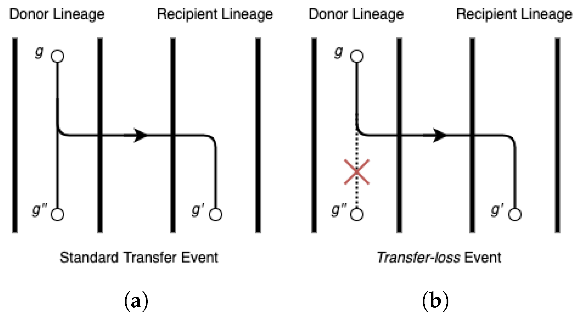
(Transfer-Loss ($\mathbb{TL}$)). A transfer-loss ($\mathbb{TL}$) event occurs when the descendants of the donor species lose all copies derived from the transferred gene.

Figure 1 provides an illustration of a $\mathbb{TL}$ event and a detailed discussion occurs in Section 2.2 below. As noted earlier, $\mathbb{TL}$ events were also explicitly defined and handled in [3,16].

Definition 2

(Transfer from unsampled lineage ($\mathbb{TX}$)). A transfer from unsampled lineage ($\mathbb{TX}$) event occurs when the donor species is not represented in the species tree.

In this work, unsampled lineages are representative any lineage not present in the species tree, including those that are extinct. We refer to transfer events that are neither $\mathbb{TL}$ events nor $\mathbb{TX}$ events as $\mathbb{T}$ events. Thus, $\mathbb{T}$ represents the “standard” transfer event type that is modeled by default in existing DTL reconciliation models.

2.2. Transfer-Loss Events

As shown in Figure 1, a $\mathbb{TL}$ event is equivalent to a standard transfer event with the exception that the donor lineage thereafter loses all copies derived from the gene that was transferred. $\mathbb{TL}$ events were first defined by Doyon et al. and implemented in their DTL reconciliation framework and software Mowgli [3]. The software ecceTERA [16] later inherited the same reconciliation framework. No other parsimony-based DTL reconciliation framework can currently handle $\mathbb{TL}$ events. Note that $\mathbb{TL}$ events do not represent a distinct biological event type; instead, they are simply standard transfer events followed later by one or more loss events that result in the donor lineage losing all copies derived from the gene that was transferred. Thus, the only reason to explicitly define $\mathbb{TL}$ events and distinguish them from standard transfer events is that most DTL reconciliation models and algorithms are not able to correctly handle evolutionary scenarios involving $\mathbb{TL}$ events. This difficulty in handling $\mathbb{TL}$ events stems from the fact that $\mathbb{TL}$ events are unary; unlike standard transfer events, they do not result in a bifurcation in the gene tree topology. Thus, there does not exist any node in the input gene tree that can represent a $\mathbb{TL}$ event. However, the DTL reconciliation model can be easily adapted to allow for $\mathbb{TL}$ events by explicitly augmenting edges in the input gene tree with additional nodes, referred to as hidden nodes. Each such hidden node simply subdivides the edge that they are augmented to, resulting in a non-binary node with a single child. This property allows hidden nodes to represent possible $\mathbb{TL}$ events, as the unary property is kept intact. More formally:

Definition 3

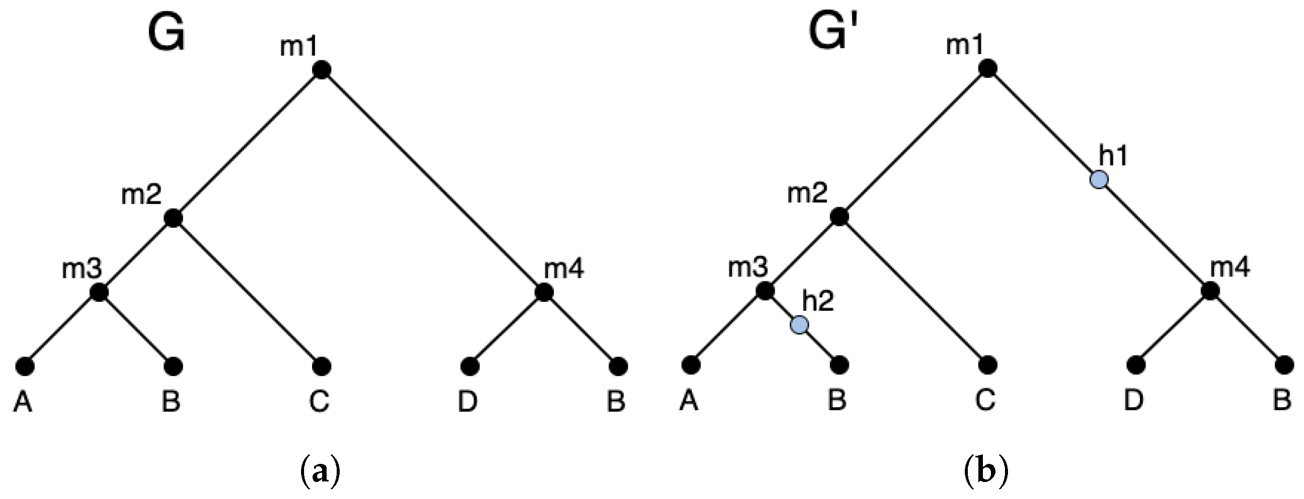
(Augmented gene tree and hidden nodes). Given a gene tree $\mathit{G}$, an augmented gene tree ${\mathit{G}}^{\prime }$ is defined to be the tree obtained from $\mathit{G}$ by (i) selecting a subset of edges $A\subseteq E\left(\mathit{G}\right)$, and (ii) subdividing each edge in A by a hidden node such that each edge $(\mathit{g},{\mathit{g}}^{\prime })\in A$ is replaced by the two edges $(\mathit{g},h)$ and $(h,{\mathit{g}}^{\prime })$, where h is a new hidden node.

Figure 2 shows an example of an augmented gene tree. The hidden nodes in an augmented gene tree can be used to represent $\mathbb{TL}$ events. Thus, under the DTLx reconciliation framework, the reconciled gene tree is in fact a reconciled augmented gene tree, where each hidden node shown on that augmented gene tree represents a $\mathbb{TL}$ event.

2.3. Transfers from Unsampled Lineages

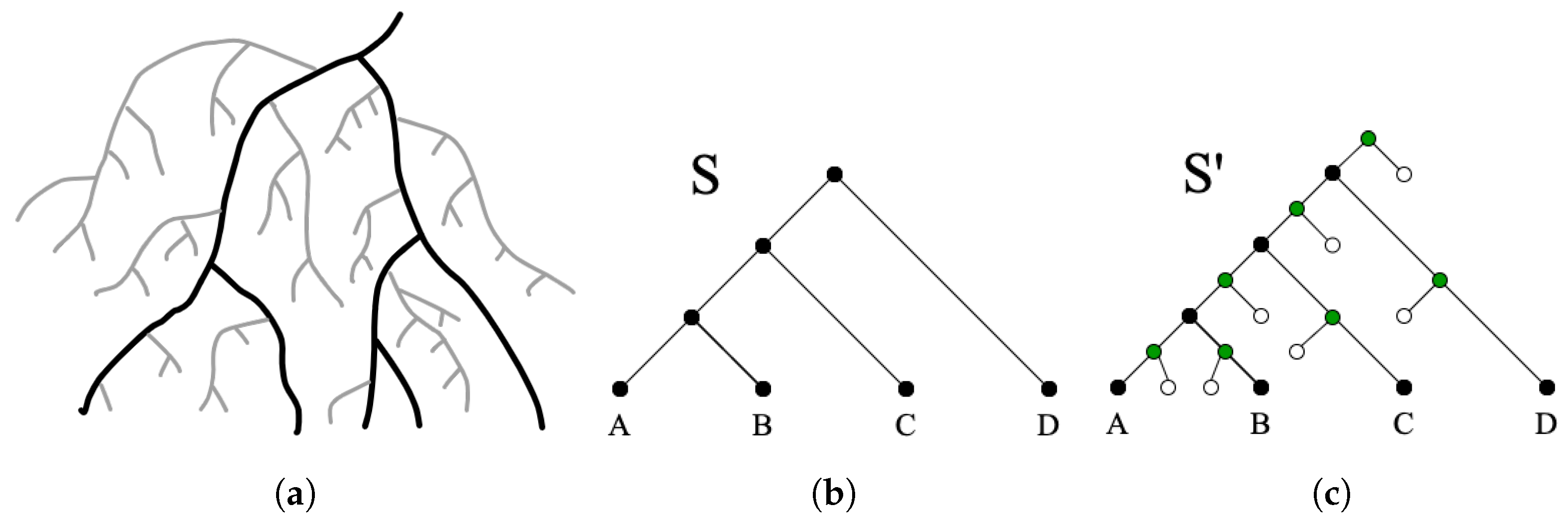
In most cases, it is difficult or impossible to achieve complete taxon sampling for the group of species under consideration. Unsampled taxa/lineages in the species tree can affect the accuracy of DTL reconciliation since transfers may have occurred from unsampled to sampled lineages. Even with complete taxon sampling, the species represented on a species tree are only those that have surviving descendant species. It is well-understood that the vast majority of species that have ever existed have gone extinct without leaving surviving descendants. This is depicted in Figure 3a. It is reasonable to expect that such extinct species lineages would have engaged in gene transfer with the species that are represented in the “visible” species tree [10]. However, conventional DTL reconciliation algorithms do not explicitly model transfers from such unsampled lineages (with the exception of [10,16], which include a simple mechanism to allow for such transfers).

We will show how transfers from unsampled species can be detected and correctly handled by appropriately augmenting the input species tree with additional edges that represent unsampled lineages and then leveraging $\mathbb{TL}$ events to allow for transfers from these additional edges to the rest of the species tree. Formally, we define the augmented species tree, denoted ${\mathit{S}}^{\prime }$, as follows:

Definition 4

(Augmented species tree and extra nodes, leaves, and edges). Given the species tree $\mathit{S}$, the augmented species tree ${\mathit{S}}^{\prime }$ is defined to be the tree obtained from $\mathit{S}$ by (i) subdividing each edge in $\mathit{E}\left(S\right)$ by a new extra node such that each edge $(s,s^{\prime })\in \mathit{E}\left(S\right)$ is replaced by the two edges $(s,e)$ and $(e,s^{\prime })$, where e is the new extra node, and connecting e by an edge to a new extra leaf, and (ii) creating a new root node r and connecting r by an edge to $\mathit{rt}\left(\mathit{S}\right)$ and by another edge to a new extra leaf. Each edge of ${\mathit{S}}^{\prime }$ connecting an extra node with an extra leaf is called an extra edge.

Figure 3c show an example of an augmented species tree. We use $\mathcal{X}\left({\mathit{S}}^{\prime }\right)$ to denote the set of all extra leaves in ${\mathit{S}}^{\prime }$. The extra edges in ${\mathit{S}}^{\prime }$ represent unsampled lineages and the new DTLx model allows for transfers to originate from these extra edges of ${\mathit{S}}^{\prime }$, and any transfer that originates at an extinct edge is labeled as a $\mathbb{TX}$ event.

2.4. DTLx Reconciliation

A DTLx reconciliation of $\mathit{G}$ and $\mathit{S}$ shows how a suitably augmented version ${\mathit{G}}^{\prime }$ of $\mathit{G}$ evolved inside the augmented species tree ${\mathit{S}}^{\prime }$ through speciation, gene duplication, transfer, $\mathbb{TL}$, $\mathbb{TX}$, and loss events. A formal definition of DTLx reconciliation appears below and it specifies what constitutes a biologically valid DTLx reconciliation of $\mathit{G}$ and $\mathit{S}$.

Definition 5

(DTLx Reconciliation). A DTLx reconciliation for $\mathit{G}$ and $\mathit{S}$ is an eleven-tuple $\langle \mathcal{L},{\mathit{G}}^{\prime },{\mathit{S}}^{\prime },\mathcal{M},\Sigma ,\Delta ,\Theta ,{\Theta }_L,{\Theta }_X,\Xi ,\tau \rangle$, where $\mathcal{L}:\mathit{Le}\left(\mathit{G}\right)\stackrel{}{\to }\mathit{Le}\left(\mathit{S}\right)$ represents the leaf mapping from $\mathit{G}$ to $\mathit{S}$, ${\mathit{G}}^{\prime }$ denotes the augmented gene tree, ${\mathit{S}}^{\prime }$ denotes the augmented species tree, $\mathcal{M}$: $\mathit{V}\left({\mathit{G}}^{\prime }\right)\to \mathit{V}\left({\mathit{S}}^{\prime }\right)$ maps each node of ${\mathit{G}}^{\prime }$ to a node of ${\mathit{S}}^{\prime }$, the sets Σ, Δ, Θ, ${\Theta }_L$, and ${\Theta }_X$ partition $\mathit{I}\left({\mathit{G}}^{\prime }\right)$ into speciation, duplication, $\mathbb{T}$, $\mathbb{TL}$, and $\mathbb{TX}$ events, respectively; Ξ is the subset of $\mathit{E}\left({\mathit{G}}^{\prime }\right)$ that represents transfer edges, and $\tau :\Theta \cup {\Theta }_L\cup {\Theta }_X\stackrel{}{\to }\mathit{V}\left({\mathit{S}}^{\prime }\right)$ specifies the recipient species for each transfer event, subject to the following constraints:

Augmented gene tree constraint

• $\mathit{G}$ can be obtained from ${\mathit{G}}^{\prime }$ by suppressing each node of ${\mathit{G}}^{\prime }$ with exactly one child.

Mapping constraints

2.

If $\mathit{g}\in \mathit{Le}\left({\mathit{G}}^{\prime }\right)$, then $\mathcal{M}\left(\mathit{g}\right)$ = $\mathcal{L}\left(\mathit{g}\right)$.

3.

If $\mathit{g}\in \mathit{I}\left(\mathit{G}\right)\cap \mathit{I}\left({\mathit{G}}^{\prime }\right)$ (i.e., g is not a hidden node of ${\mathit{G}}^{\prime }$) and ${\mathit{g}}^{\prime }$ and ${\mathit{g}}^{″}$ denote the children of $\mathit{g}$ in ${\mathit{G}}^{\prime }$, then,

(a)

$\mathcal{M}\left(\mathit{g}\right){\cancel{<}}_{{\mathit{S}}^{\prime }}\mathcal{M}\left({\mathit{g}}^{\prime }\right)$, and $\mathcal{M}\left(\mathit{g}\right){\cancel{<}}_{{\mathit{S}}^{\prime }}\mathcal{M}\left({\mathit{g}}^{″}\right)$,

(b)

At least one of $\mathcal{M}\left({\mathit{g}}^{\prime }\right)$ and $\mathcal{M}\left({\mathit{g}}^{″}\right)$ is a descendant of $\mathcal{M}\left(\mathit{g}\right)$.

4.

If $\mathit{g}\in \mathit{I}\left({\mathit{G}}^{\prime }\right)\setminus \mathit{I}\left(\mathit{G}\right)$ (i.e., g is a hidden node of ${\mathit{G}}^{\prime }$) and ${\mathit{g}}^{\prime }$ denotes it’s unique child, then $\mathcal{M}\left(\mathit{g}\right)$ and $\mathcal{M}\left({\mathit{g}}^{\prime }\right)$ are incomparable.

Event constraints

5.

Given any edge $(\mathit{g},{\mathit{g}}^{\prime })\in \mathit{E}\left({\mathit{G}}^{\prime }\right)$, $(\mathit{g},{\mathit{g}}^{\prime })\in \Xi$ if and only if $\mathcal{M}\left(\mathit{g}\right)$ and $\mathcal{M}\left({\mathit{g}}^{\prime }\right)$ are incomparable.

6.

If $\mathit{g}\in \mathit{I}\left(\mathit{G}\right)\cap \mathit{I}\left({\mathit{G}}^{\prime }\right)$ and ${\mathit{g}}^{\prime }$ and ${\mathit{g}}^{″}$ denote the children of $\mathit{g}$ in ${\mathit{G}}^{\prime }$, then,

(a)

$\mathit{g}\in \Sigma$ only if $\mathcal{M}\left(\mathit{g}\right)=\mathit{lca}(\mathcal{M}\left({\mathit{g}}^{\prime }\right),\mathcal{M}\left({\mathit{g}}^{″}\right))$ and $\mathcal{M}\left({\mathit{g}}^{\prime }\right)$ and $\mathcal{M}\left({\mathit{g}}^{″}\right)$ are incomparable,

(b)

$\mathit{g}\in \Delta$ only if $\mathcal{M}\left(\mathit{g}\right){\ge }_{{\mathit{S}}^{\prime }}\mathit{lca}(\mathcal{M}\left({\mathit{g}}^{\prime }\right)$, $\mathcal{M}\left({\mathit{g}}^{″}\right))$,

(c)

$\mathit{g}\in \Theta$ if and only if either $(\mathit{g},{\mathit{g}}^{\prime })\in \Xi$ or $(\mathit{g},{\mathit{g}}^{″})\in \Xi$,

(d)

If $\mathit{g}\in \Theta$ and $(\mathit{g},{\mathit{g}}^{\prime })\in \Xi$, then $\mathcal{M}\left(\mathit{g}\right)$ and $\tau \left(\mathit{g}\right)$ must be incomparable and $\mathcal{M}\left({\mathit{g}}^{\prime }\right)$ must be a descendant of $\tau \left(\mathit{g}\right)$, i.e., $\mathcal{M}\left({\mathit{g}}^{\prime }\right){\le }_{{\mathit{S}}^{\prime }}\tau \left(\mathit{g}\right)$.

7.

If $\mathit{g}\in \mathit{I}\left({\mathit{G}}^{\prime }\right)\setminus \mathit{I}\left(\mathit{G}\right)$ and ${\mathit{g}}^{\prime }$ denotes it’s unique child, then,

(a)

$\mathit{g}\in {\Theta }_L\cup {\Theta }_X$, and $(\mathit{g},{\mathit{g}}^{\prime })\in \Xi$

(b)

$\mathcal{M}\left(\mathit{g}\right)$ and $\tau \left(\mathit{g}\right)$ are incomparable, and $\mathcal{M}\left({\mathit{g}}^{\prime }\right){\le }_{{\mathit{S}}^{\prime }}\tau \left(\mathit{g}\right)$

(c)

$\mathit{g}\in {\Theta }_X$ if and only if $\mathcal{M}\left(\mathit{g}\right)\in \mathcal{X}\left({\mathit{S}}^{\prime }\right)$.

Constraint 1 specifies how the gene tree can be augmented with hidden nodes so that any inferred $\mathbb{TL}$ and $\mathbb{TX}$ events can be shown in the final reconciliation. Constraint 2 ensures that the mapping $\mathcal{M}$ is consistent with the leaf-mapping $\mathcal{L}$. Because $\mathit{Le}\left({\mathit{G}}^{\prime }\right)$ is equivalent to $\mathit{Le}\left(\mathit{G}\right)$, the leaf mappings of ${\mathit{G}}^{\prime }$ into ${\mathit{S}}^{\prime }$ must be equivalent to those of $\mathit{G}$ into $\mathit{S}$. Constraints 3a and 4 impose on $\mathcal{M}$ the temporal constraints implied by ${\mathit{S}}^{\prime }$. Constraint 3b implies that any non-hidden internal node in ${\mathit{G}}^{\prime }$ may represent at most one transfer event. Constraint 5 determines the edges of ${\mathit{G}}^{\prime }$ that are $\mathbb{T}$, $\mathbb{TL}$, or $\mathbb{TX}$ edges. Constraints 6a–c state the conditions under which a non-hidden internal node of ${\mathit{G}}^{\prime }$ may represent a speciation, duplication, and transfer, respectively. Constraint 6d specifies which species may be designated as the recipient species for any given $\mathbb{T}$ event. Constraint 7a ensures that only those hidden nodes that represent a valid $\mathbb{TL}$ or $\mathbb{TX}$ event can appear in ${\mathit{G}}^{\prime }$. Constraint 7b specifies which species may be designated as the recipient species for any given $\mathbb{TL}$ or $\mathbb{TX}$ event. Finally, Constraint 7c differentiates $\mathbb{TL}$ from $\mathbb{TX}$ events and requires that any $\mathbb{TX}$ event must originate along an extra edge (representing unsampled lineages) of the augmented species tree.

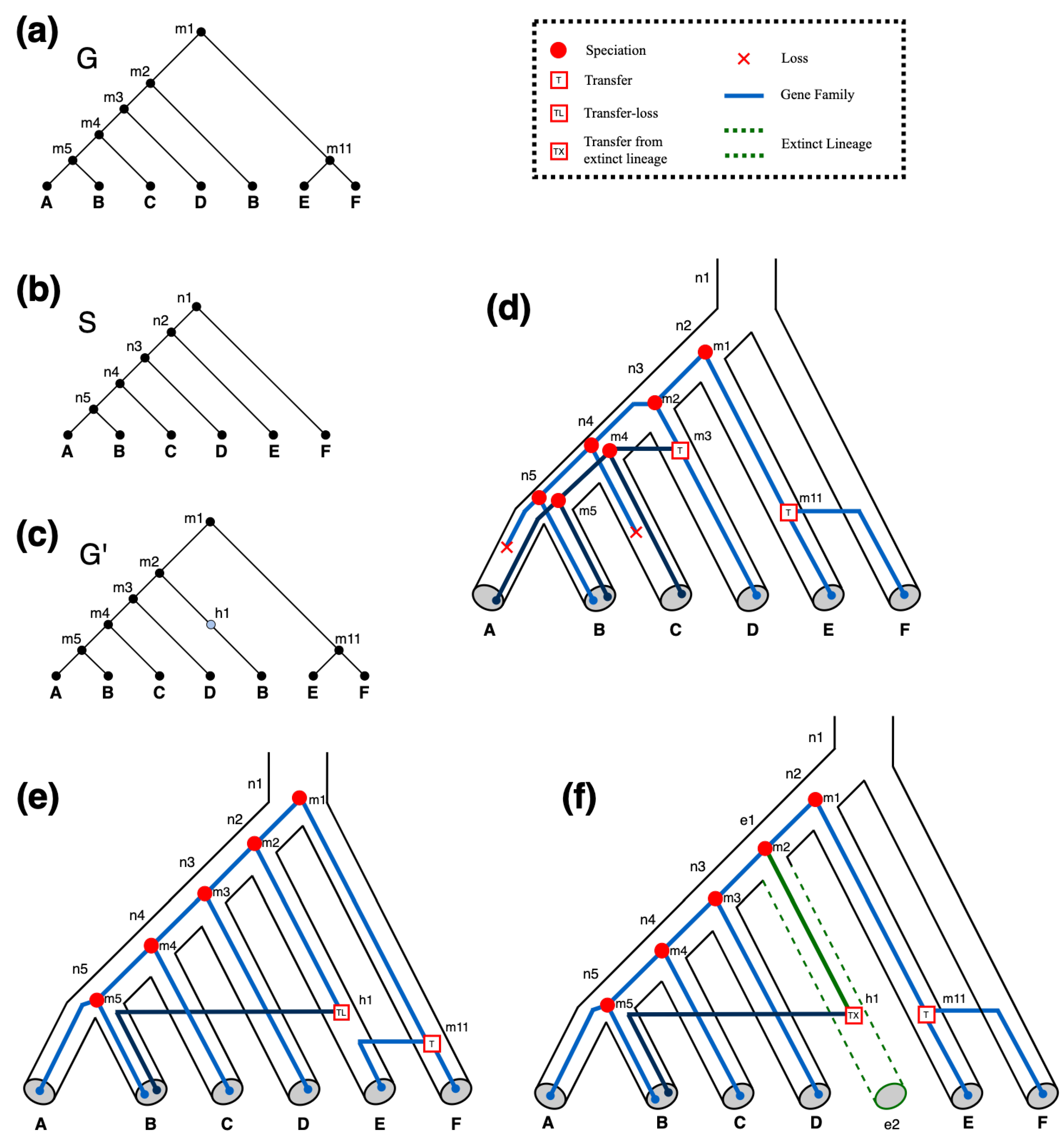
Figure 4 shows examples of DTLx reconciliations and illustrates how allowing for $\mathbb{TL}$ and $\mathbb{TX}$ events can lead to improved reconciliations.

Given a DTLx reconciliation $\alpha$, one can directly count the minimum number of gene losses implied by $\alpha$ similarly as under the DTL reconciliation model [7], but with two additional considerations: First, any losses associated with $\mathbb{TL}$ and $\mathbb{TX}$ events (i.e., associated with hidden nodes of ${\mathit{G}}^{\prime }$) must be appropriately counted. Furthermore, second, losses must be counted using the original, unaugmented species tree $\mathit{S}$, rather than using ${\mathit{S}}^{\prime }$, except in cases where a gene tree node maps to an extra leaf. Specifically, to count the minimum number of losses that occur along an edge $(\mathit{g},{\mathit{g}}^{\prime })$ of the gene tree, we must count the number of non-extra species lineages in the species tree that branch off from the path $\mathcal{M}\left(\mathit{g}\right){\to }_{{\mathit{S}}^{\prime }}\mathcal{M}\left({\mathit{g}}^{\prime }\right)$, and also account for any extra edges along the path. To facilitate this counting, we define the loss-distance between two nodes $x,y\in \mathit{V}\left({\mathit{S}}^{\prime }\right)$, where $y{\le }_{{\mathit{S}}^{\prime }}x$, denoted $d_{{\mathit{S}}^{\prime }}(x,y)$, as follows:

$$d_{{\mathit{S}}^{\prime }}(x,y)=\left\{\begin{array}{cc}0,\hfill & \mathrm{if}x=y,\hfill \\ \left|\right\{e:e\in \mathit{E}\left(\mathit{S}\right)\mathrm{and}e\mathrm{fully}\mathrm{or}\mathrm{partially}\mathrm{overlaps}\mathrm{with}\mathrm{the}\mathrm{path}x{\to }_{{\mathit{S}}^{\prime }}y\left\}\right|,\hfill & \mathrm{if}y\notin \mathcal{X}\left({\mathit{S}}^{\prime }\right)\hfill \\ \left|\right\{e:e\in \mathit{E}\left(\mathit{S}\right)\mathrm{and}e\mathrm{fully}\mathrm{or}\mathrm{partially}\mathrm{overlaps}\mathrm{with}\mathrm{the}\mathrm{path}x{\to }_{{\mathit{S}}^{\prime }}y\left\}\right|+1,\hfill & \mathrm{otherwise}\hfill \end{array}\right.$$

For example, in the species tree ${\mathit{S}}^{\prime }$ shown in Figure 4f, $d_{{\mathit{S}}^{\prime }}(n_2,B)=4$ and $d_{{\mathit{S}}^{\prime }}(n_2,e_2)=2$.

Definition 6

(Losses). Given a DTLx reconciliation $\alpha =\langle \mathcal{L},{\mathit{G}}^{\prime },{\mathit{S}}^{\prime },\mathcal{M},\Sigma ,\Delta ,\Theta ,{\Theta }_L,{\Theta }_X,\Xi ,\tau \rangle$ for $\mathit{G}$ and $\mathit{S}$, let $\mathit{g}\in \mathit{V}\left({\mathit{G}}^{\prime }\right)$ and $\{{\mathit{g}}^{\prime },{\mathit{g}}^{″}\}=\mathit{Ch}\left(\mathit{g}\right)$ if $\mathit{g}\in \mathit{I}\left(\mathit{G}\right)\cap \mathit{I}\left({\mathit{G}}^{\prime }\right)$, and $\left\{{\mathit{g}}^{\prime }\right\}=\mathit{Ch}\left(\mathit{g}\right)$ otherwise. The minimum number of losses $Los{s}_{\alpha }\left(\mathit{g}\right)$ at node $\mathit{g}$ (or, more accurately, the minimum number of losses incurred along the child edge(s) of $\mathit{g}$) is defined to be:

• $d_{{\mathit{S}}^{\prime }}(\mathcal{M}\left(\mathit{g}\right),\mathcal{M}\left({\mathit{g}}^{\prime }\right))+d_{{\mathit{S}}^{\prime }}(\mathcal{M}\left(\mathit{g}\right),\left(\mathcal{M}\left({\mathit{g}}^{″}\right)\right)-2,\mathrm{if}\hspace{0.17em}\mathit{g}\in \Sigma$;
• $d_{{\mathit{S}}^{\prime }}(\mathcal{M}\left(\mathit{g}\right),\mathcal{M}\left({\mathit{g}}^{\prime }\right))+d_{{\mathit{S}}^{\prime }}(\mathcal{M}\left(\mathit{g}\right),\mathcal{M}\left({\mathit{g}}^{″}\right))\hspace{0.17em}\mathrm{if}\hspace{0.17em}\mathit{g}\in \Delta$;
• $d_{{\mathit{S}}^{\prime }}(\mathcal{M}\left(\mathit{g}\right),\mathcal{M}\left({\mathit{g}}^{″}\right))+d_{{\mathit{S}}^{\prime }}(\tau \left(\mathit{g}\right),\mathcal{M}\left({\mathit{g}}^{\prime }\right))\mathrm{if}(\mathit{g},{\mathit{g}}^{\prime })\in \Xi \mathrm{and}\mathit{g}\in \Theta ,\mathrm{and}$;
• $d_{{\mathit{S}}^{\prime }}(\tau \left(\mathit{g}\right),\mathcal{M}\left({\mathit{g}}^{\prime }\right)\mathrm{if}(\mathit{g},{\mathit{g}}^{\prime })\in \Xi ,\mathrm{and}\hspace{0.17em}\mathit{g}\in {\Theta }_L\mathrm{or}\hspace{0.17em}\mathit{g}\in {\Theta }_X$.

The total number of losses associated with reconciliation α, denoted ${\mathrm{Loss}}_{\alpha }$, is defined to be ${\sum }_{\mathit{g}\in \mathit{I}\left({\mathit{G}}^{\prime }\right)}{\mathrm{Loss}}_{\alpha }\left(\mathit{g}\right)$.

Note that the implicit gene loss (of the donor’s copy of the gene) associated with $\mathbb{TL}$ or $\mathbb{TX}$ events is not counted in the definition of losses above. Instead, $\mathbb{TL}$ and $\mathbb{TX}$ events can be assigned a higher event cost than a standard transfer event (see next paragraph) to account for these implicit losses.

In the DTLx reconciliation framework, each event other than speciation (which is considered a null event) is assigned a positive cost. Let $P_{\Delta }$, $P_{\Theta }$, $P_{\mathbb{TL}}$, $P_{\mathbb{TX}}$, and $P_{loss}$ denote the costs associated with duplication, transfer, $\mathbb{TL}$, $\mathbb{TX}$, and loss events, respectively. The reconciliation cost of a DTLx reconciliation $\alpha$ of $\mathit{G}$ and $\mathit{S}$ is then defined as follows.

Definition 7

(Reconciliation cost). Given a DTLx reconciliation $\alpha =\langle \mathcal{L},{\mathit{G}}^{\prime },{\mathit{S}}^{\prime },\mathcal{M},\Sigma ,\Delta ,\Theta ,{\Theta }_L,{\Theta }_X,\Xi ,\tau \rangle$ for $\mathit{G}$ and $\mathit{S}$, the reconciliation cost associated with α is the total cost of all events invoked by α. Specifically, the reconciliation cost is given by $P_{\Delta }\times |\Delta |+P_{\Theta }\times |\Theta |+P_{\mathbb{TL}}\times |{\Theta }_L|+P_{\mathbb{TX}}\times \left|{\Theta }_X\right|+P_{loss}\times {\mathrm{Loss}}_{\alpha }$.

Given $\mathit{G}$ and $\mathit{S}$, along with specific event costs, the computational objective is to find a DTLx reconciliation of $\mathit{G}$ and $\mathit{S}$ with minimum reconciliation cost (i.e., a most parsimonious DTLx reconciliation of $\mathit{G}$ and $\mathit{S}$). This yields the following problem statement.

Problem 1

(Optimal DTLx reconciliation (O-DTLx) problem). Given $\mathit{G}$ and $\mathit{S}$, along with $P_{\Delta }$, $P_{\Theta }$, $P_{\mathbb{TL}}$, $P_{\mathbb{TX}}$, and $P_{loss}$, the O-DTLx problem is to find a DTLx reconciliation for $\mathit{G}$ and $\mathit{S}$ with minimum reconciliation cost.

It is well-understood that there can exist a very large number of optimal DTL reconciliations for any given gene tree and species tree and that this number can grow exponentially in the sizes of the input trees [11,12]. One of the most efficient and widely used approaches for handling multiple optima and exploring the diversity of optimal reconciliations is to generate optimal reconciliations uniformly at random from the space of all optimal reconciliations [11,17]. Such random sampling for the efficient exploration of the space of multiple optima and makes it possible to distinguish well-supported and poorly-supported aspects of an optimal reconciliation. This motivates the following problem statement.

Problem 2

(Optimal DTLx reconciliation sampling (O-DTLx-Sampling) problem). Given $\mathit{G}$ and $\mathit{S}$, along with $P_{\Delta }$, $P_{\Theta }$, $P_{\mathbb{TL}}$, $P_{\mathbb{TX}}$, and $P_{loss}$, let $\mathcal{O}$ denote the set of all optimal DTLx reconciliations for $\mathit{G}$ and $\mathit{S}$ (i.e., with minimum reconciliation cost). The O-DTLx-Sampling problem is to compute an optimal DTLx reconciliation from $\mathcal{O}$ in such a way that each DTLx reconciliation in $\mathcal{O}$ has an equal probability of being computed.

We provide efficient algorithms for both the above problems in the following section.

3. Materials and Methods

Our algorithms for computing and sampling optimal DTLx reconciliations build upon corresponding dynamic programming algorithms for computing and sampling optimal DTL reconciliations as described in [7,11]. These algorithms for DTL reconciliation perform a nested post-order traversal of the gene tree and species tree and compute, at each step, an optimal solution to a subproblem. Specifically, given any $\mathit{g}\in \mathit{V}\left(\mathit{G}\right)$ and $\mathit{s}\in \mathit{V}\left(\mathit{S}\right)$, the subproblem $c(\mathit{g},\mathit{s})$ is defined to be cost of an optimal DTL reconciliation of the subtree $\mathit{G}\left(\mathit{g}\right)$ with $\mathit{S}$ under the constraint that $\mathit{g}$ maps to $\mathit{s}$. As shown in [7], optimal solutions for these subproblems can be efficiently computed based on previously computed optimal solutions for smaller subproblems, and the final optimal reconciliation cost for $\mathit{G}$ and $\mathit{S}$ is then simply ${min}_{\mathit{s}\in \mathit{V}\left(\mathit{S}\right)}c(\mathit{rt}\left(\mathit{G}\right),\mathit{s})$.

Adapting this approach to computing DTLx reconciliations requires several modifications and extensions to the basic dynamic programming framework. In particular, (i) hidden nodes in the augmented gene tree must be handled differently in the dynamic programming framework than the other nodes, (ii) mappings to extra leaves in the species tree must be handled differently than mappings to other nodes, and (iii) the new evolutionary events $\mathbb{TL}$ and $\mathbb{TX}$ must be integrated into the cost calculations performed within the dynamic programming framework.

Recall that a DTLx reconciliation of $\mathit{G}$ and $\mathit{S}$ is a reconciliation between an augmented gene tree ${\mathit{G}}^{\prime }$ and the augmented species tree ${\mathit{S}}^{\prime }$. Accordingly, our algorithms for computing optimal DTLx reconciliations perform a nested post order traversal of a fully augmented gene tree, denoted ${\mathit{G}}^{″}$, and the augmented species tree ${\mathit{S}}^{\prime }$. This fully augmented gene tree is defined as follows:

Definition 8

(Fully augmented gene tree). Given a gene tree $\mathit{G}$, the fully augmented gene tree, denoted ${\mathit{G}}^{″}$, is defined to be the tree obtained from $\mathit{G}$ by subdividing each edge in $\mathit{E}\left(\mathit{G}\right)$ by a hidden node such that each edge $(\mathit{g},{\mathit{g}}^{\prime })\in \mathit{E}\left(\mathit{G}\right)$ is replaced by the two edges $(\mathit{g},h)$ and $(h,{\mathit{g}}^{\prime })$, where h is a new hidden node.

The fully augmented gene tree ${\mathit{G}}^{″}$ thus contains all possible hidden nodes and allows the algorithms to consider the possibility of $\mathbb{TL}$ and $\mathbb{TX}$ events occurring along each edge of G. Hidden nodes of ${\mathit{G}}^{″}$ that are not ultimately labeled as representing a $\mathbb{TL}$ or $\mathbb{TX}$ event are suppressed to yield the final augmented gene tree ${\mathit{G}}^{\prime }$.

Next, we present our algorithm for the O-DTLx problem.

3.1. An $O\left(mn\right)$-Time Algorithm for O-DTLx

Following along the lines of the previous dynamic programming framework described above, we define the core subproblem of dynamic programming algorithm as follows: Given any $\mathit{g}\in \mathit{V}\left({\mathit{G}}^{″}\right)$ and $\mathit{s}\in \mathit{V}\left({\mathit{S}}^{\prime }\right)$, we define $c(\mathit{g},\mathit{s})$ to be cost of an optimal DTLx reconciliation of the subtree ${\mathit{G}}^{″}\left(\mathit{g}\right)$ with ${\mathit{S}}^{\prime }$ under the constraint that $\mathit{g}$ maps to $\mathit{s}$. Note that the hidden nodes of ${\mathit{G}}^{″}$ that are not used in a DTLx reconciliation do not contribute to the reconciliation cost of that reconciliation. These unused hidden nodes can therefore be trimmed out at the end to yield the final augmented gene tree ${\mathit{G}}^{\prime }$. Thus, in accordance with the definition of DTLx reconciliation, the optimal reconciliation cost of reconciling $\mathit{G}$ and $\mathit{S}$ is given by ${min}_{\mathit{s}\in \mathit{V}\left({\mathit{S}}^{\prime }\right)}c(\mathit{rt}\left({\mathit{G}}^{″}\right),\mathit{s})$.

For each non-hidden internal node $\mathit{g}$ of ${\mathit{G}}^{″}$, i.e., if $\mathit{g}\in \mathit{I}\left({\mathit{G}}^{″}\right)\cap \mathit{I}\left(\mathit{G}\right)$, we also define the following restricted subproblems: (i) $c_{\Sigma }(\mathit{g},\mathit{s})$ denotes the cost of an optimal reconciliation of ${\mathit{G}}^{″}\left(\mathit{g}\right)$ with ${\mathit{S}}^{\prime }$ under the constraint that $\mathit{g}$ maps to $\mathit{s}$ and $\mathit{g}\in \Sigma$. (ii) $c_{\Delta }(\mathit{g},\mathit{s})$ denotes the cost of an optimal reconciliation of ${\mathit{G}}^{″}\left(\mathit{g}\right)$ with ${\mathit{S}}^{\prime }$ under the constraint that $\mathit{g}$ maps to $\mathit{s}$ and $\mathit{g}\in \Delta$. Furthermore, (iii) $c_{\Theta }(\mathit{g},\mathit{s})$ denotes the cost of an optimal reconciliation of ${\mathit{G}}^{″}\left(\mathit{g}\right)$ with ${\mathit{S}}^{\prime }$ under the constraint that $\mathit{g}$ maps to $\mathit{s}$ and $\mathit{g}\in \Theta$.

Recall that only the hidden nodes of ${\mathit{G}}^{″}$ can represent $\mathbb{TL}$ and $\mathbb{TX}$ events. Accordingly, for each hidden node $\mathit{g}$ of ${\mathit{G}}^{″}$, i.e., if $\mathit{g}\in I\left({\mathit{G}}^{″}\right)\setminus \mathit{I}\left(\mathit{G}\right)$, we define the following restricted subproblems: (i) $c_{{\Theta }_L}(\mathit{g},\mathit{s})$ denotes the cost of an optimal reconciliation of ${\mathit{G}}^{″}\left(g\right)$ with ${\mathit{S}}^{\prime }$ under the constraint that $\mathit{g}$ maps to $\mathit{s}$ and $\mathit{g}\in {\Theta }_L$. (ii) $c_{{\Theta }_X}(\mathit{g},\mathit{s})$ denotes the cost of an optimal reconciliation of ${\mathit{G}}^{\prime \prime }\left(\mathit{g}\right)$ with ${\mathit{S}}^{\prime }$ under the constraint that $\mathit{g}$ maps to $\mathit{s}$ and $\mathit{g}\in {\Theta }_X$.

The algorithm executes a nested post order traversal of ${\mathit{G}}^{″}$ and ${\mathit{S}}^{\prime }$ to compute the value of $c(\mathit{g},\mathit{s})$ for each $\mathit{g}$ and $\mathit{s}$. The base cases for the dynamic programming table are initialized as follows:

$$c(\mathit{g},\mathit{s})=\left\{\begin{array}{cc}0\hfill & \mathrm{if}\mathit{g}\in \mathit{Le}\left({\mathit{G}}^{″}\right)\mathrm{and}\mathit{s}=\mathcal{L}\left(\mathit{g}\right),\hfill \\ \infty \hfill & \mathrm{if}\mathit{g}\in \mathit{Le}\left({\mathit{G}}^{″}\right)\mathrm{and}\mathit{s}\ne \mathcal{L}\left(\mathit{g}\right).\hfill \end{array}\right.$$

(1)

For internal nodes of ${\mathit{G}}^{″}$, $c(\mathit{g},\mathit{s})$ can be computed based on the values of the restricted subproblems, defined above, as follows:

$$c(\mathit{g},\mathit{s})=\left\{\begin{array}{cc}min\{c_{\Sigma }({\mathit{g}}^{\prime },\mathit{s}),c_{\Delta }({\mathit{g}}^{\prime },\mathit{s}),c_{\Theta }({\mathit{g}}^{\prime },\mathit{s}),c_{{\Theta }_L}(\mathit{g},\mathit{s}),c_{{\Theta }_X}(\mathit{g},\mathit{s})\}\hfill & \mathrm{if}\mathit{g}\in \mathit{I}\left({\mathit{G}}^{″}\right)\setminus \mathit{I}\left(\mathit{G}\right),\hfill \\ min\{c_{\Sigma }(\mathit{g},\mathit{s}),c_{\Delta }(\mathit{g},\mathit{s}),c_{\Theta }(\mathit{g},\mathit{s})\}\hfill & \mathrm{otherwise},\hfill \end{array}\right.$$

(2)

where ${\mathit{g}}^{\prime }$ denotes the unique child of $\mathit{g}$ in the case where $\mathit{g}$ is a hidden node (i.e., $\mathit{g}\in \mathit{I}\left({\mathit{G}}^{″}\right)\setminus \mathit{I}\left(\mathit{G}\right)$).

Note that, when $\mathit{g}\in \mathit{I}\left({\mathit{G}}^{″}\right)\cap \mathit{I}\left(\mathit{G}\right)$, the value of $c(\mathit{g},\mathit{s})$ is the minimum of the restricted subproblem values computed at $\mathit{g}$ and ${\mathit{g}}^{\prime }$. Essentially, if $c(\mathit{g},\mathit{s})$ equals $c_{\Sigma }(\mathit{g},\mathit{s})$, $c_{\Delta }(\mathit{g},\mathit{s})$, or $c_{\Theta }(\mathit{g},\mathit{s})$, then it means that the hidden node $\mathit{g}$ is not required (i.e., it need not represent any event) in an optimal reconciliation corresponding to that value of $c(\mathit{g},\mathit{s})$.

For each $\mathit{g}$ and $\mathit{s}$, optimal values for the applicable restricted subproblems represented by $c_{\Sigma }(\mathit{g},\mathit{s})$, $c_{\Delta }(\mathit{g},\mathit{s})$, $c_{\Theta }(\mathit{g},\mathit{s})$, $c_{{\Theta }_L}(\mathit{g},\mathit{s})$, and $c_{{\Theta }_X}(\mathit{g},\mathit{s})$ can be computed based on previously computed values of $c(·,·)$ as shown below. For ease of presentation and to help compute these values more efficiently, we also define, for each $\mathit{g}\in \mathit{V}\left({\mathit{G}}^{″}\right)$ and $\mathit{s}\in \mathit{V}\left({\mathit{S}}^{\prime }\right)$, the following:

$$\begin{array}{cc}\hfill \mathit{in}(\mathit{g},\mathit{s})& =\underset{\mathit{x}\in \mathit{V}\left({\mathit{S}}^{\prime }\left(\mathit{s}\right)\right)}{min}\{P_{loss}·d_{{\mathit{S}}^{\prime }}(\mathit{s},\mathit{x})+c(\mathit{g},\mathit{x})\}\hfill \\ \hfill \mathit{out}(\mathit{g},\mathit{s})& =\underset{\mathit{x}\in \mathit{V}\left({\mathit{S}}^{\prime }\right)\mathrm{incomparable}\mathrm{to}\mathit{s}}{min}c(\mathit{g},\mathit{x})\hfill \\ \hfill \mathit{inAlt}(\mathit{g},\mathit{s})& =\underset{\mathit{x}\in \mathit{V}\left({\mathit{S}}^{\prime }\left(\mathit{s}\right)\right)}{min}c(\mathit{g},\mathit{x}).\hfill \end{array}$$

Now, consider any $\mathit{g}\in \mathit{I}\left({\mathit{G}}^{″}\right)\cap \mathit{I}\left(\mathit{G}\right)$, and let $\{{\mathit{g}}^{\prime },{\mathit{g}}^{″}\}={\mathit{Ch}}_{{\mathit{G}}^{″}}\left(\mathit{g}\right)$. If $\mathit{s}\notin \mathit{Le}\left({\mathit{S}}^{\prime }\right)$ then let $\{{\mathit{s}}^{\prime },{\mathit{s}}^{″}\}={\mathit{Ch}}_{{\mathit{S}}^{\prime }}\left(\mathit{s}\right)$. Then,

$$c_{\Sigma }(\mathit{g},\mathit{s})=\left\{\begin{array}{cc}\infty \hfill & \mathrm{if}\mathit{s}\in \mathit{Le}\left({\mathit{S}}^{\prime }\right),\hfill \\ min\{\mathit{in}({\mathit{g}}^{\prime },{\mathit{s}}^{\prime })+\mathit{in}({\mathit{g}}^{″},{\mathit{s}}^{″}),\mathit{in}({\mathit{g}}^{″},{\mathit{s}}^{\prime })+\mathit{in}({\mathit{g}}^{\prime },{\mathit{s}}^{″})\}\hfill & \mathrm{otherwise},\hfill \end{array}\right.$$

(3)

$$c_{\Delta }(\mathit{g},\mathit{s})=\left\{\begin{array}{cc}{P}_{\Delta }+c({\mathit{g}}^{\prime },\mathit{s})+c({\mathit{g}}^{″},\mathit{s})\hfill & \mathrm{if}\mathit{s}\in \mathit{Le}\left({\mathit{S}}^{\prime }\right),\hfill \\ P_{\Delta }+\mathit{in}({\mathit{g}}^{\prime },\mathit{s})+\mathit{in}({\mathit{g}}^{″},\mathit{s})\hfill & \mathrm{otherwise},\hfill \end{array}\right.$$

(4)

and

$$c_{\Theta }(\mathit{g},\mathit{s})=\left\{\begin{array}{cc}\infty \hfill & \mathrm{if}\mathit{s}=\mathit{rt}\left({\mathit{S}}^{\prime }\right),\hfill \\ P_{\Theta }+min\{\mathit{in}({\mathit{g}}^{\prime },\mathit{s})+\mathit{out}({\mathit{g}}^{″},\mathit{s}),\mathit{in}({\mathit{g}}^{″},\mathit{s})+\mathit{out}({\mathit{g}}^{\prime },\mathit{s})\}\hfill & \mathrm{otherwise}.\hfill \end{array}\right.$$

(5)

Similarly, if $\mathit{g}\in \mathit{I}\left({\mathit{G}}^{″}\right)\setminus \mathit{I}\left(\mathit{G}\right)$, i.e., $\mathit{g}$ is a hidden node, and ${\mathit{g}}^{\prime }$ represents the unique child of $\mathit{g}$ in ${\mathit{G}}^{″}$, then,

$$c_{{\Theta }_L}(\mathit{g},\mathit{s})=\left\{\begin{array}{cc}\infty \hfill & \mathrm{if}\mathit{s}=\mathit{rt}\left({\mathit{S}}^{\prime }\right)\mathrm{or}\mathit{s}\in \mathcal{X}\left({\mathit{S}}^{\prime }\right),\hfill \\ P_{\mathbb{TL}}+\mathit{out}({\mathit{g}}^{\prime },\mathit{s})\hfill & \mathrm{otherwise},\hfill \end{array}\right.$$

(6)

and

$$c_{{\Theta }_X}(\mathit{g},\mathit{s})=\left\{\begin{array}{cc}\infty \hfill & \mathrm{if}\mathit{s}=\mathit{rt}\left({\mathit{S}}^{\prime }\right)\mathrm{or}\mathit{s}\notin \mathcal{X}\left({\mathit{S}}^{\prime }\right),\hfill \\ P_{\mathbb{TX}}+\mathit{out}({\mathit{g}}^{\prime },\mathit{s})\hfill & \mathrm{otherwise},\hfill \end{array}\right.$$

(7)

The O-DTLx problem can now be easily solved using dynamic programming based on Equations (1)–(7). The pseudocode given in Algorithm 1, i.e., Algorithm Compute-O-DTLx, shows how this can be done within $O\left(mn\right)$ time by efficiently computing the values of $\mathit{in}(·,·)$, $\mathit{out}(·,·)$, and $\mathit{inAlt}(·,·)$.

Observe that Algorithm 1 only computes the optimal reconciliation cost. However, as with any dynamic programming algorithm, it is straightforward to compute an actual reconciliation that achieves this optimal reconciliation cost through backtracking. Furthermore, observe that it is trivial to “trim down” any reconciliation of ${\mathit{G}}^{″}$ and ${\mathit{S}}^{\prime }$ constructed through backtracking by simply removing any hidden node in ${\mathit{G}}^{″}$ that is not assigned a $\mathbb{TL}$ or $\mathbb{TX}$ event in that reconciliation. This would yield the augmented gene tree ${\mathit{G}}^{\prime }$, along with its reconciliation with ${\mathit{S}}^{\prime }$, as required by the definition of DTLx reconciliation (Definition 5).

Theorem 1.

The O-DTLx problem can be solved in $O\left(mn\right)$ time, where $m=\left|\mathit{Le}\right(G\left)\right|$ and $n=\left|\mathit{Le}\right(S\left)\right|$.

Proof. 

It suffices to show that Algorithm 1 correctly computes the value of $c(\mathit{g},\mathit{s})$, for each $\mathit{g}\in \mathit{V}\left({\mathit{G}}^{\prime }\right)$ and $\mathit{s}\in \mathit{V}\left({\mathit{S}}^{\prime }\right)$, within $O\left(mn\right)$ time.

Correctness: We will show that the values of $\mathit{in}(\mathit{g},\mathit{s})$, $\mathit{inAlt}(\mathit{g},\mathit{s})$, $\mathit{out}(\mathit{g},\mathit{s})$, ${\mathit{c}}_{\Sigma }(\mathit{g},\mathit{s})$, ${\mathit{c}}_{\Delta }(\mathit{g},\mathit{s})$, ${\mathit{c}}_{\Theta }(\mathit{g},\mathit{s})$, ${\mathit{c}}_{{\Theta }_L}(\mathit{g},\mathit{s})$, and ${\mathit{c}}_{{\Theta }_X}(\mathit{g},\mathit{s})$ are computed correctly for each $\mathit{g}$ and $\mathit{s}$ where applicable. For each $\mathit{g}\in \mathit{Le}\left({\mathit{G}}^{\prime }\right)$, consider the values of $\mathit{in}(\mathit{g},\mathit{s})$, $\mathit{inAlt}(\mathit{g},\mathit{s})$, $\mathit{out}(\mathit{g},\mathit{s})$ and $\mathit{c}(\mathit{g},\mathit{s})$. These values are assigned correctly in accordance with their definitions during the execution of the ‘for’ loop in Steps 8–11. These values serve as the base case of our inductive argument.

Consider the case when $\mathit{g}\in \mathit{I}\left({\mathit{G}}^{″}\right)\setminus \mathit{I}\left(\mathit{G}\right)$, and ${\mathit{g}}^{\prime }=\mathit{Ch}\left(\mathit{g}\right)$. By the induction hypothesis, we may assume that the values of $\mathit{in}({\mathit{g}}^{\prime },\mathit{x})$, $\mathit{inAlt}({\mathit{g}}^{\prime },\mathit{x})$, and $\mathit{c}({\mathit{g}}^{\prime },\mathit{x})$ have been computed correctly for each $\mathit{x}\in \mathit{V}\left({\mathit{S}}^{\prime }\right)$. Given the values of $\mathit{inAlt}({\mathit{g}}^{\prime },\mathit{x})$, the values of $\mathit{out}({\mathit{g}}^{\prime },\mathit{x})$ must also be computed correctly during the execution of the ‘for’ loop in Steps 33–35. Observe that the values of ${\mathit{c}}_{{\Theta }_L}(\mathit{g},\mathit{s})$, ${\mathit{c}}_{{\Theta }_X}(\mathit{g},\mathit{s})$, and $\mathit{c}(\mathit{g},\mathit{s})$, for any $\mathit{s}\in \mathit{V}\left({\mathit{S}}^{\prime }\right)$, are computed using these previously computed values in accordance with Equations (2), (6), and (7), which, in turn, are based directly on the definitions of the corresponding events given in Definition 5. Thus, these values are all computed correctly. Once the values $\mathit{c}(\mathit{g},\mathit{s})$ are computed correctly, the remaining values of $\mathit{in}(\mathit{g},\mathit{s})$, $\mathit{inAlt}(\mathit{g},\mathit{s})$, and $\mathit{out}(\mathit{g},\mathit{s})$ would also be assigned correctly in Steps 18–22 and Steps 33–35, in accordance with their definitions.

Now, consider the case when $\mathit{g}\in \mathit{I}\left({\mathit{G}}^{″}\right)\cap \mathit{I}\left(\mathit{G}\right)$, and $\{{\mathit{g}}^{\prime },{\mathit{g}}^{″}\}=\mathit{Ch}\left(\mathit{g}\right)$. By the induction hypothesis, we may again assume that the values of $\mathit{in}({\mathit{g}}^{\prime },\mathit{x})$, $\mathit{in}({\mathit{g}}^{″},\mathit{x})$, $\mathit{inAlt}({\mathit{g}}^{\prime },\mathit{x})$, $\mathit{inAlt}({\mathit{g}}^{″},\mathit{x})$, $\mathit{c}({\mathit{g}}^{\prime },\mathit{x})$, and $\mathit{c}({\mathit{g}}^{″},\mathit{x})$ have been computed correctly for each $\mathit{x}\in \mathit{V}\left({\mathit{S}}^{\prime }\right)$. Given the values of $\mathit{inAlt}({\mathit{g}}^{\prime },\mathit{x})$ and $\mathit{inAlt}({\mathit{g}}^{″},\mathit{x})$, the values of $\mathit{out}({\mathit{g}}^{\prime },\mathit{x})$ and $\mathit{out}({\mathit{g}}^{″},\mathit{x})$ must also be computed correctly during the execution of the ‘for’ loop in Steps 33–35. Observe that the values of ${\mathit{c}}_{\Sigma }(\mathit{g},\mathit{s})$, ${\mathit{c}}_{\Delta }(\mathit{g},\mathit{s})$, ${\mathit{c}}_{\Theta }(\mathit{g},\mathit{s})$, and $\mathit{c}(\mathit{g},\mathit{s})$, for any $\mathit{s}\in \mathit{V}\left({\mathit{S}}^{\prime }\right)$, are computed using these previously computed values in accordance with Equations (2)–(5), which, in turn, are based directly on the definitions of the corresponding events given in Definition 5. Thus, these values are all computed correctly. Once the values $\mathit{c}(\mathit{g},\mathit{s})$ are computed correctly, the remaining values of $\mathit{in}(\mathit{g},\mathit{s})$, $\mathit{inAlt}(\mathit{g},\mathit{s})$ and $\mathit{out}(\mathit{g},\mathit{s})$ would also be assigned correctly in Steps 28–32 and Steps 33–35, in accordance with their definitions.

Induction completes the proof.

Time complexity: The time complexity of the Algorithm is dominated by the nested ‘for’ loops in Steps 12 through 35 that perform the nexted post-order traversal of the gene and species tree. It is easy to verify that each step within these nested ‘for’ loops requires only $O\left(1\right)$ time. Thus, the time complexity of Algorithm 1 is $O\left(mn\right)$.

Algorithm 1 Compute-O-DTLx($\mathit{G},\mathit{S},\mathcal{L},P_{\Sigma },P_{\Delta },P_{\Theta },P_{\mathbb{TL}},P_{\mathbb{TX}},P_{loss}$)

1: Initialize ${\mathit{G}}^{″}$ and ${\mathit{S}}^{\prime }$ as outlined earlier.

2: for each $\mathit{g}\in \mathit{V}\left({\mathit{G}}^{″}\right)$ and $\mathit{s}\in \mathit{V}\left({\mathit{S}}^{\prime }\right)$ do

3:  Initialize $c(\mathit{g},\mathit{s})$, $\mathit{in}(\mathit{g},\mathit{s})$, $\mathit{out}(\mathit{g},\mathit{s})$, and $\mathit{inAlt}(\mathit{g},\mathit{s})$ to ∞.

4:  if $\mathit{g}\in \mathit{I}\left({\mathit{G}}^{″}\right)\cap \mathit{I}\left(\mathit{G}\right)$ then

5:   Initialize $c_{\Sigma }(\mathit{g},\mathit{s})$, $c_{\Delta }(\mathit{g},\mathit{s})$, and $c_{\Theta }(\mathit{g},\mathit{s})$ to ∞.

6:  if $\mathit{g}\in \mathit{I}\left({\mathit{G}}^{″}\right)\setminus \mathit{I}\left(\mathit{G}\right)$ then

7:   Initialize $c_{{\Theta }_L}(\mathit{g},\mathit{s})$ and $c_{{\Theta }_X}(\mathit{g},\mathit{s})$ to ∞.

8: for each $\mathit{g}\in \mathit{Le}\left({\mathit{G}}^{″}\right)$ do

9:   Initialize $c(\mathit{g},\mathcal{L}(\mathit{g}\left)\right)$ to 0

10:  For each $\mathit{s}{\ge }_{{\mathit{S}}^{\prime }}\mathcal{L}\left(\mathit{g}\right)$, initialize $\mathit{in}(\mathit{g},\mathit{s})$ to $P_{loss}·d_{{\mathit{S}}^{\prime }}(\mathit{s},\mathcal{L}\left(\mathit{g}\right))$ and $\mathit{inAlt}(\mathit{g},\mathit{s})$ to 0.

11:  For each $\mathit{s}\in V\left({\mathit{S}}^{\prime }\right)$ incomparable to $\mathcal{L}\left(\mathit{g}\right)$, assign $\mathit{out}(\mathit{g},\mathit{s})=0$.

12: for each $\mathit{g}\in \mathit{I}\left({\mathit{G}}^{″}\right)$ in post-order do

13:  for each $\mathit{s}\in \mathit{V}\left({\mathit{S}}^{\prime }\right)$ in post-order do

14:   if $\mathit{g}\in \mathit{I}\left({\mathit{G}}^{″}\right)\setminus \mathit{I}\left(\mathit{G}\right)$ then

15:    Let ${\mathit{g}}^{\prime }$ denote the unique child of $\mathit{g}$ in ${\mathit{G}}^{″}$.

16:    Compute $c_{{\Theta }_L}(\mathit{g},\mathit{s})$ and $c_{{\Theta }_X}(\mathit{g},\mathit{s})$ according to Equations (6) and (7), respectively.

17:    Compute $c(\mathit{g},\mathit{s})$ according to Equation (2).

18:    if $\mathit{s}\in \mathit{Le}\left({\mathit{S}}^{\prime }\right)$ then

19:     $\mathit{in}(\mathit{g},\mathit{s})=\mathit{inAlt}(\mathit{g},\mathit{s})=c(\mathit{g},\mathit{s})$.

20:    else

21:     $\mathit{inAlt}(\mathit{g},\mathit{s})=min\{c(\mathit{g},\mathit{s}),\mathit{inAlt}(\mathit{g},{\mathit{s}}^{\prime }),\mathit{inAlt}(\mathit{g},{\mathit{s}}^{″})\}$.

22:     If s is an extra node then $\mathit{in}(\mathit{g},\mathit{s})=min\{c(\mathit{g},\mathit{s}),\mathit{in}(\mathit{g},{\mathit{s}}^{\prime })+P_{loss},\mathit{in}(\mathit{g},{\mathit{s}}^{″})+P_{loss}\}$. If s is not an extra node then $\mathit{in}(\mathit{g},\mathit{s})=min\{c(\mathit{g},\mathit{s}),\mathit{in}(\mathit{g},{\mathit{s}}^{\prime }),\mathit{in}(\mathit{g},{\mathit{s}}^{″})\}$.

23:   if $\mathit{g}\in \mathit{I}\left({\mathit{G}}^{″}\right)\cap \mathit{I}\left(\mathit{G}\right)$ then

24:    Let $\{{\mathit{g}}^{\prime },{\mathit{g}}^{″}\}={\mathit{Ch}}_{{\mathit{G}}^{\prime }}\left(\mathit{g}\right)$.

25:    If $\mathit{s}\notin \mathit{Le}\left({\mathit{S}}^{\prime }\right)$ then let $\{{\mathit{s}}^{\prime },{\mathit{s}}^{″}\}={\mathit{Ch}}_{{\mathit{S}}^{\prime }}\left(\mathit{s}\right)$.

26:    Compute $c_{\Sigma }(\mathit{g},\mathit{s})$, $c_{\Delta }(\mathit{g},\mathit{s})$, and $c_{\Theta }(\mathit{g},\mathit{s})$ according to Equations (3), (4), and (5), respectively.

27:    Compute $c(\mathit{g},\mathit{s})$ according to Equation (2).

28:    if $\mathit{s}\in \mathit{Le}\left({\mathit{S}}^{\prime }\right)$ then

29:     $\mathit{in}(\mathit{g},\mathit{s})=\mathit{inAlt}(\mathit{g},\mathit{s})=c(\mathit{g},\mathit{s})$.

30:    else

31:     $\mathit{inAlt}(\mathit{g},\mathit{s})=min\{\mathit{c}(\mathit{g},\mathit{s}),\mathit{inAlt}(\mathit{g},{\mathit{s}}^{\prime }),\mathit{inAlt}(\mathit{g},{\mathit{s}}^{″})\}$.

32:     If s is an extra node then $\mathit{in}(\mathit{g},\mathit{s})=min\{c(\mathit{g},\mathit{s}),\mathit{in}(\mathit{g},{\mathit{s}}^{\prime })+P_{loss},\mathit{in}(\mathit{g},{\mathit{s}}^{″})+P_{loss}\}$. If s is not an extra node then $\mathit{in}(\mathit{g},\mathit{s})=min\{c(\mathit{g},\mathit{s}),\mathit{in}(\mathit{g},{\mathit{s}}^{\prime }),\mathit{in}(\mathit{g},{\mathit{s}}^{″})\}$.

33:  for each $\mathit{s}\in \mathit{I}\left({\mathit{S}}^{\prime }\right)$ in pre-order do

34:   Let $\{{\mathit{s}}^{\prime },{\mathit{s}}^{″}\}={\mathit{Ch}}_{{\mathit{S}}^{\prime }}\left(\mathit{s}\right)$.

35:   $\mathit{out}(\mathit{g},{\mathit{s}}^{\prime })=min\{\mathit{out}(\mathit{g},\mathit{s}),\mathit{inAlt}(\mathit{g},{\mathit{s}}^{″})\}$, and $\mathit{out}(\mathit{g},{\mathit{s}}^{″})=min\left\{\mathit{out}(\mathit{g},\mathit{s})\mathit{inAlt}(\mathit{g},{\mathit{s}}^{\prime })\right\}$.

36: Return ${min}_{\mathit{s}\in \mathit{V}\left({\mathit{S}}^{\prime }\right)}c(\mathit{rt}\left({\mathit{G}}^{″}\right),\mathit{s})$.

3.2. An $O\left(m{n}^2\right)$-Time Algorithm for O-DTLx-Sampling

As with any dynamic programming algorithm, Algorithm 1 can be easily extended to keep track of all optimal choices at each step of the algorithm and to use these optimal choices to (1) compute all possible optimal reconciliations, and/or (2) perform probabilistic backtracking to sample from the space of optimal reconciliations uniformly at random. Since there is often a very large number of optimal reconciliations [11,12], making it infeasible to enumerate all possible optimal reconciliations in practice, we will show how to perform probabilistic backtracking to sample from the space of optimal DTLx reconciliations uniformly at random. Our sampling algorithm builds on the very similar sampling algorithm previously developed for DTL reconciliation [11] and implemented in RANGER-DTL 2.0 [17]. Given the similarity with [11], here we only provide a high level description of the overall approach, focusing primarily on describing the handling of hidden nodes and $\mathbb{TL}$ and $\mathbb{TX}$ events.

The key idea that enables uniform random sampling is to keep track of the number of optimal DTLx reconciliations associated with each subproblem. Accordingly, we define the following: Given any $\mathit{g}\in \mathit{V}\left({\mathit{G}}^{″}\right)$ and $\mathit{s}\in {\mathit{S}}^{\prime }$, let $\mathit{N}(\mathit{g},\mathit{s})$ denote the number of optimal reconciliations for ${\mathit{G}}^{″}\left(\mathit{g}\right)$ and ${\mathit{S}}^{\prime }$ such that $\mathit{g}$ maps to $\mathit{s}$. Thus, $\mathit{N}(\mathit{g},\mathit{s})$ is the number of distinct DTLx reconciliations of ${\mathit{G}}^{″}\left(\mathit{g}\right)$ and ${\mathit{S}}^{\prime }$, under the constraint that $\mathit{g}$ maps to $\mathit{s}$, that have a reconciliation cost of exactly $\mathit{c}(\mathit{g},\mathit{s})$. These $\mathit{N}(\mathit{g},\mathit{s})$ values can be easily computed alongside the corresponding $\mathit{c}(\mathit{g},\mathit{s})$ values using the same overall dynamic programming framework as in Algorithm 1.

Analogous to $c_{\Sigma }(\mathit{g},\mathit{s})$, $c_{\Delta }(\mathit{g},\mathit{s})$, and $c_{\Theta }(\mathit{g},\mathit{s})$, we define, for each non-hidden internal node $\mathit{g}$ of ${\mathit{G}}^{″}$ (i.e., $\mathit{g}\in \mathit{I}\left({\mathit{G}}^{″}\right)\cap \mathit{I}\left(\mathit{G}\right)$), ${\mathit{N}}_{\Sigma }(\mathit{g},\mathit{s})$, ${\mathit{N}}_{\Delta }(\mathit{g},\mathit{s})$, and ${\mathit{N}}_{\Theta }(\mathit{g},\mathit{s})$. Similarly, analogous to $c_{{\Theta }_L}(\mathit{g},\mathit{s})$ and $c_{{\Theta }_X}(\mathit{g},\mathit{s})$, we define, for each hidden node $\mathit{g}$ of ${\mathit{G}}^{″}$ (i.e., $\mathit{g}\in I\left({\mathit{G}}^{″}\right)\setminus \mathit{I}\left(\mathit{G}\right)$), ${\mathit{N}}_{{\Theta }_L}(\mathit{g},\mathit{s})$ and ${\mathit{N}}_{{\Theta }_X}(\mathit{g},\mathit{s})$.

The dynamic programming table for $\mathit{N}(·,·)$ can be initialized as follows for each $\mathit{g}\in \mathit{Le}\left({\mathit{G}}^{″}\right)$:

$$\mathit{N}(\mathit{g},\mathit{s})=\left\{\begin{array}{cc}1\hfill & \mathrm{if}\mathit{g}\in \mathit{Le}\left({\mathit{G}}^{″}\right)\mathrm{and}\mathit{s}=\mathcal{L}\left(\mathit{g}\right),\hfill \\ 0\hfill & \mathrm{if}\mathit{g}\in \mathit{Le}\left({\mathit{G}}^{″}\right)\mathrm{and}\mathit{s}\ne \mathcal{L}\left(\mathit{g}\right).\hfill \end{array}\right.$$

(8)

It is easy to see that, for internal nodes of ${\mathit{G}}^{″}$, $\mathit{N}(·,·)$ can be computed based on the values of the restricted counts defined above as follows:

$$\mathit{N}(\mathit{g},\mathit{s})=\left\{\begin{array}{cc}\sum _{x\in \{\Sigma ,\Delta ,\Theta \}\mathrm{where}{c}_x({\mathit{g}}^{\prime },\mathit{s})=c(\mathit{g},\mathit{s})}{N}_x({\mathit{g}}^{\prime },\mathit{s})+\sum _{x\in \{{\Theta }_L,{\Theta }_X\}\mathrm{where}{c}_x(\mathit{g},\mathit{s})=c(\mathit{g},\mathit{s})}{N}_x(\mathit{g},\mathit{s})\hfill & \mathrm{if}\mathit{g}\in \mathit{I}\left({\mathit{G}}^{″}\right)\setminus \mathit{I}\left(\mathit{G}\right),\hfill \\ \sum _{x\in \{\Sigma ,\Delta ,\Theta \}\mathrm{where}{c}_x(\mathit{g},\mathit{s})=c(\mathit{g},\mathit{s})}{N}_x(\mathit{g},\mathit{s})\hfill & \mathrm{otherwise},\hfill \end{array}\right.$$

(9)

where ${\mathit{g}}^{\prime }$ denotes the unique child of $\mathit{g}$ in the case where $\mathit{g}$ is a hidden node (i.e., $\mathit{g}\in \mathit{I}\left({\mathit{G}}^{″}\right)\setminus \mathit{I}\left(\mathit{G}\right)$).

Now, for any $\mathit{g}\in \mathit{I}\left({\mathit{G}}^{″}\right)\cap \mathit{I}\left(\mathit{G}\right)$, the values of ${\mathit{N}}_{\Sigma }(\mathit{g},\mathit{s})$, ${\mathit{N}}_{\Delta }(\mathit{g},\mathit{s})$, and ${\mathit{N}}_{\Theta }(\mathit{g},\mathit{s})$ can be computed exactly as described in [11] for DTL reconciliation. It therefore suffices to show how to compute the values ${\mathit{N}}_{{\Theta }_L}(\mathit{g},\mathit{s})$ and ${\mathit{N}}_{{\Theta }_X}(\mathit{g},\mathit{s})$ when $\mathit{g}$ is a hidden node.

Suppose $\mathit{g}\in \mathit{I}\left({\mathit{G}}^{″}\right)\setminus \mathit{I}\left(\mathit{G}\right)$, i.e., $\mathit{g}$ is a hidden node, and ${\mathit{g}}^{\prime }$ represents the unique child of $\mathit{g}$ in ${\mathit{G}}^{″}$. For any $\mathit{s}\in V\left({\mathit{S}}^{\prime }\right)$, let A denote the set of all mappings of ${\mathit{g}}^{\prime }$ that are optimal for $c_{{\Theta }_L}(\mathit{g},\mathit{s})$, i.e., for any $x\in A$ we must have $c_{{\Theta }_L}(\mathit{g},\mathit{s})=P_{\mathbb{TL}}+c({\mathit{g}}^{\prime },x)$. Likewise, let B denote the set of all mappings of ${\mathit{g}}^{\prime }$ that are optimal for $c_{{\Theta }_X}(\mathit{g},\mathit{s})$, i.e., for any $x\in B$ we must have $c_{{\Theta }_X}(\mathit{g},\mathit{s})=P_{\mathbb{TX}}+c({\mathit{g}}^{\prime },\mathit{x})$. The values of ${\mathit{N}}_{{\Theta }_L}(\mathit{g},\mathit{s})$ and ${\mathit{N}}_{{\Theta }_X}(\mathit{g},\mathit{s})$ can then be computed as follows:

$${\mathit{N}}_{{\Theta }_L}(\mathit{g},\mathit{s})=\sum _{x\in A}\mathit{N}({\mathit{g}}^{\prime },x),$$

(10)

and

$${\mathit{N}}_{{\Theta }_X}(\mathit{g},\mathit{s})=\sum _{x\in B}\mathit{N}({\mathit{g}}^{\prime },x).$$

(11)

Together with the equations for ${\mathit{N}}_{\Sigma }(\mathit{g},\mathit{s})$, ${\mathit{N}}_{\Delta }(\mathit{g},\mathit{s})$, and ${\mathit{N}}_{\Theta }(\mathit{g},\mathit{s})$ from [11], Equations (8)–(11) make it possible to compute all $\mathit{N}(\mathit{g},\mathit{s})$ values alongside those of $\mathit{c}(\mathit{g},\mathit{s})$ using the same nested post-order traversal used in Algorithm 1. However, as also described in [11], to compute the $\mathit{N}(\mathit{g},\mathit{s})$ values, we need to keep track of all optimal mappings for the child/children of $\mathit{g}$ that yield the optimal reconciliation cost at $\mathit{g}$. Thus, it is not possible to use the speedups enabled by precomputing the required values of $\mathit{in}(·,·)$, $\mathit{inAlt}(·,·)$, and $\mathit{out}(·,·)$, leading to an increased overall time complexity of $O\left(m{n}^2\right)$ [11]. Furthermore, once all the $\mathit{N}(·,·)$ values have been computed, it is straightforward to perform a probabilistic backtracking procedure, completely analogous to the one described in [11] for DTL reconciliation, to sample from the space of all optimal DTLx reconciliations for G and S uniformly at random. Thus, we have the following theorem.

Theorem 2.

The O-DTLx-Sampling problem can be solved in $O\left(m{n}^2\right)$ time, where $m=\left|\mathit{Le}\right(G\left)\right|$ and $n=\left|\mathit{Le}\right(S\left)\right|$.

3.3. Assigning Event Costs for $\mathbb{TL}$ and $\mathbb{TX}$

Based on analyses of simulated and biological datasets, DTL reconciliation often uses default event costs of 1, 2, and 3 for losses, duplications, and transfers, respectively, [5,16,17]. For $\mathbb{TL}$ events, it makes sense to use a cost equal to $P_{\Theta }+P_{loss}$ since a $\mathbb{TL}$ event implies one transfer and at least one loss. For $\mathbb{TX}$ events, a cost equal to that of a transfer event may be appropriate, since each $\mathbb{TX}$ event implies one transfer but not necessarily any other events (besides extinction or non-sampling). However, depending on the specific dataset being analyzed, e.g., based on the approximate age of the root of the species tree or on the extent of incomplete taxon sampling, it may make sense to assign a slightly higher cost for $\mathbb{TX}$ events, such as a cost equal to $P_{\Theta }+P_{loss}$.

Theoretically, observe that if $P_{\mathbb{TX}}=P_{\Theta }$ then, for every optimal DTLx reconciliation that invokes a transfer event, there exists a distinct and equally optimal DTLx reconciliation in which that transfer event is substituted by an equivalent $\mathbb{TX}$ event. Thus, assigning $P_{\mathbb{TX}}$ to be strictly greater than $P_{\Theta }$ may make it easier to distinguish between transfer and $\mathbb{TX}$ events.

4. Results

To assess the accuracy and impact of our new DTLx reconciliation framework, we implemented our ODTLx-Sampling algorithm and applied it to both simulated and real datasets. We describe the results of this experimental evaluation below.

4.1. Results on Simulated Datasets

We used simulated datasets to systematically evaluate the accuracy of DTLx reconciliations and to compare its accuracy and functionality against ecceTERA, the only other parsimony-based reconciliation model that handles $\mathbb{TL}$ and $\mathbb{TX}$ events. Our implementation is built upon the open-source RANGER-DTL software package [17] and we refer to the new software implementation as RANGER-DTLx.

We used the recently developed phylogenetic tree simulation software ZOMBI [29] to evolve simulated gene trees with known ground-truth evolutionary histories containing explicit transfers from extinct lineages. ZOMBI tracks species lineages that eventually go extinct and allows for such lineages to participate in horizontal gene transfer events before going extinct. In our analysis, we simulated two datasets, each consisting of 500 gene tree/species tree pairs. Note that each of these 500 pairs consist of a unique (i.e., different) species tree and gene tree, where each of the species trees has exactly 50 taxa. The specific parameters used to generate the datasets are shown in

Table 1. Parameter settings used to generate simulated datasets using Zombi.

	Gene Tree Parameters			Species Tree Parameters
Dataset	Duplication Rate	Transfer Rate	Loss Rate	Birth Rate	Extinction Rate	# Taxa (Leaves)
1	0.022	0.04	0.01	0.1	0.025	50
2	0.020	0.06	0.008	0.1	0.032	50

. Notably, Dataset-2 has a higher rate of transfers and more $\mathbb{TX}$ events in the gene trees due to a higher extinction rate. For increased realism, the transfer rate was split evenly between additive and replacing transfers.

The final gene trees, obtained after pruning out all gene lineages with no surviving gene descendants, had, on average, 152.5 leaves, 11.6 duplications, 18.1 transfers, 3.0 $\mathbb{TX}$ events, and 121.7 speciations for Dataset-1, and 180.3 leaves, 10.5 duplications, 26.7 transfers, 5.7 $\mathbb{TX}$ events, and 142 speciations for Dataset-2. For reference, the unpruned gene trees showed on average, for Dataset-1, 16.1 losses and 42 extinctions, and for Dataset-2, 24.2 losses and 67.4 extinctions. Thus, Datasets 1 and 2 correspond to low and moderate rates, respectively, of the relevant evolutionary events.

We used these two simulated datasets to address the following three questions: (i) Does using DTLx reconciliation, i.e., RANGER-DTLx, improve upon the overall accuracy of DTL reconciliation in the presence of $\mathbb{TX}$ events? (ii) How well do RANGER-DTLx and ecceTERA detect $\mathbb{TX}$ events? Furthermore, (iii) How do RANGER-DTLx and ecceTERA compare in their ability to detect the phylogenetic location of the extinct donor of a $\mathbb{TX}$ event?

Comparing accuracies of DTL and DTLx reconciliation. Since both RANGER-DTLx and ecceTERA can account for additional evolutionary scenarios that cannot be correctly handled in traditional DTL reconciliation, it is reasonable to expect that both RANGER-DTLx and ecceTERA should result in greater overall reconciliation accuracy than traditional DTL reconciliation. We therefore applied RANGER-DTLx, ecceTERA, and RANGER-DTL (which implements the traditional DTL reconciliation framework) to both simulated datasets and evaluated the overall accuracies of the resulting reconciliations. Note that, for a fair comparison, we only compared reconciliation accuracy across the nodes present on the input gene trees, without inclusion of any hidden nodes inferred by RANGER-DTLx.

For an inferred reconciliation $\alpha$, let ${\Sigma }_{\alpha }$, ${\Delta }_{\alpha }$, ${\Theta }_{\alpha }$, ${\mathcal{M}}_{\alpha }$, and ${\tau }_{\alpha }$ denote the sets of speciation nodes, duplication nodes, standard transfer nodes, mappings for internal nodes of G, and transfer recipients for standard transfers, respectively. The sets ${\Sigma }_T$, ${\Delta }_T$, ${\Theta }_T$, ${\mathcal{M}}_T$, and ${\tau }_T$ are defined analogously for the ground truth reconciliation $\beta$. Overall accuracy is quantified through the following three metrics:

$$\begin{array}{cc}\hfill \mathrm{Event}\mathrm{accuracy}& =\frac{|{\Sigma }_{\alpha }\cap {\Sigma }_{\beta }|+|{\Delta }_{\alpha }\cap {\Delta }_{\beta }|+|{\Theta }_{\alpha }\cap {\Theta }_{\beta }|}{\left|\mathit{I}\right(\mathit{G}\left)\right|}\hfill \\ \hfill \mathrm{Mapping}\mathrm{accuracy}& =\frac{\left|\right\{g:{\mathcal{M}}_{\alpha }\left(\mathit{g}\right)={\mathcal{M}}_{\beta }\left(\mathit{g}\right)\left\}\right|}{\left|\mathit{I}\right(\mathit{G}\left)\right|}\hfill \\ \hfill \mathrm{Recipient}\mathrm{accuracy}& =\frac{\left|\right\{g:\mathit{g}\in {\Theta }_{\alpha }\cap {\Theta }_{\beta }\mathrm{and}{\tau }_{\alpha }\left(\mathit{g}\right)={\tau }_{\beta }\left(\mathit{g}\right)\left\}\right|}{|{\Theta }_{\alpha }\cap {\Theta }_{\beta }|}\hfill \end{array}$$

To account for multiple optimal reconciliations, we used the standard approach of assigning the most well supported mapping and event type for each of the three methods/software. Specifically, 100 random optimal reconciliations were sampled for each gene tree/species tree pair, for both RANGER-DTLx and RANGER-DTL, and each gene tree node was assigned the most frequently observed mapping and event type among the 100 samples [11]. A similar procedure was followed for ecceTERA, but based on the reconciliation graph computed by ecceTERA [12], rather than on uniform random sampling.

Recall that, unlike ecceTERA, our DTLx reconciliation framework allows for independent assignment of $\mathbb{TL}$ and $\mathbb{TX}$ event costs. We therefore tried two different costs for $\mathbb{TX}$ events in all our experiments: 3 and 4. We fixed the cost of a $\mathbb{TL}$ event at 4. The costs for other events were fixed as follows for all three methods: Loss cost = 1, duplication cost = 2, and transfer cost = 3, which correspond to the defaults used in RANGER-DTL and ecceTERA. Based on these costs, ecceTERA automatically assigns $\mathbb{TL}$ events a cost of 4 (equivalent to one transfer plus one loss), and $\mathbb{TX}$ events a cost of 3 (equivalent to one transfer event).

The results of our analysis appear in

Table 2. Overall reconciliation accuracy. Average reconciliation accuracy, in terms of mapping accuracy and event assignment accuracy, is shown for each method. Event/mapping accuracy for a given input gene tree is calculated as the total number of correct events/mappings divided by the total number of internal nodes in that gene tree. The table also shows the accuracy of inferred recipients for transfer events. This recipient accuracy for each gene tree is calculated as the total number of correctly identified recipients divided by the total number of correctly identified transfers. Results are averaged across the 500 gene tree/species tree pairs in each dataset.

Dataset-1
	Event Accuracy	Mapping Accuracy	Recipient Accuracy
RANGER-DTL	0.961	0.937	0.682
RANGER-DTLx, $P_{\mathbb{TX}}=4$	0.961	0.939	0.697
RANGER-DTLx, $P_{\mathbb{TX}}=3$	0.917	0.895	0.716
ecceTERA	0.961	0.937	0.704
Dataset-2
	Event Accuracy	Mapping Accuracy	Recipient Accuracy
RANGER-DTL	0.944	0.912	0.623
RANGER-DTLx, $P_{\mathbb{TX}}=4$	0.944	0.912	0.637
RANGER-DTLx, $P_{\mathbb{TX}}=3$	0.894	0.861	0.670
ecceTERA	0.945	0.910	0.650

. As the table shows, RANGER-DTL, RANGER-DTLx with $\mathbb{TX}$ cost 4, and ecceTERA have nearly indistinguishable reconciliation accuracies across both datasets, while RANGER-DTLx with $\mathbb{TX}$ cost 3 shows slightly worse event and mapping accuracies but slightly better recipient accuracy. These results suggest that models that account for $\mathbb{TL}$ and $\mathbb{TX}$ events may not result in improved overall reconciliation accuracy compared to traditional DTL reconciliation, at least for low to moderate rates of $\mathbb{TX}$ events as in our datasets. Importantly, these results also show that allowing for $\mathbb{TL}$ and $\mathbb{TX}$ events does not worsen reconciliation accuracy, even when the rate of $\mathbb{TX}$ events is low (Dataset-1).

Accuracy of $\mathbb{TX}$ event detection. Next, we assessed how well RANGER-DTLx and ecceTERA can infer ground-truth $\mathbb{TX}$ events. We labelled transfers from unsampled lineages as ground truth $\mathbb{TX}$ events if, in the event log generated by ZOMBI, the gene survives in an extant lineage but the original copy goes extinct. While the original name of the internal gene tree node representing the extinct gene is absent from the input gene tree, we can verify if either method correctly detects this transfer by looking for a $\mathbb{TX}$ event with the same recipient as the ground truth transfer.

We first assessed how well $\mathbb{TX}$ events were detected, in terms of precision and recall, in a single random optimal reconciliation computed by each method.

Table 3. Accuracy of $\mathbb{TX}$ event detection. The precision and recall for $\mathbb{TX}$ events inferred by each method are shown. A single optimal reconciliation is used per gene tree, and results are aggregated across all 500 gene tree/species tree pairs in each dataset.

	Dataset-1			Dataset-2
	$\mathbb{TX}$s Returned	Recall	Precision	$\mathbb{TX}$s Returned	Recall	Precision
RANGER-DTLx, $P_{\mathbb{TX}}=4$	29	0.33%	17.24%	51	0.52%	29.41%
RANGER-DTLx, $P_{\mathbb{TX}}=3$	4515	30.12%	9.97%	6740	29.94%	12.73%
ecceTERA	413	2.61%	9.44%	668	3.16%	13.62%

shows the results of this analysis, which reveals several interesting insights. First, and perhaps most strikingly, we find that none of the methods shows high precision in detecting $\mathbb{TX}$ events, with ecceTERA and RANGER-DTLx with $\mathbb{TX}$ cost 3 both showing 10% precision in the two datasets, and RANGER-DTLx with $\mathbb{TX}$ cost 4 showing much higher, but still relatively low, precision of 17.24% in Dataset-1 and 29.41% in Dataset-2. Second, we find that RANGER-DTLx with $\mathbb{TX}$ cost 3 and ecceTERA, despite using effectively the same event costs, differ dramatically in the number of $\mathbb{TX}$ events they infer. For example, for Dataset-1, ecceTERA infers only 413 $\mathbb{TX}$ events across all 500 gene trees with recall and precision of 2.61% and 9.44%, respectively, and RANGER-DTLx with $\mathbb{TX}$ cost 3 infers 4515 $\mathbb{TX}$ events with recall and precision of 30.12% and 9.97%. Furthermore, third, these results show that there is a clear tradeoff between sensitivity and precision of $\mathbb{TX}$ event inference and suggest that RANGER-DTLx with $\mathbb{TX}$ cost 4 should be the method of choice for $\mathbb{TX}$ event inference if precision is more important than recall, while RANGER-DTLx with $\mathbb{TX}$ cost 3 should be used if recall is more important than precision. This experiment also highlights the utility of allowing for a user-specifiable cost for $\mathbb{TX}$ events as permitted under our model but not under ecceTERA.

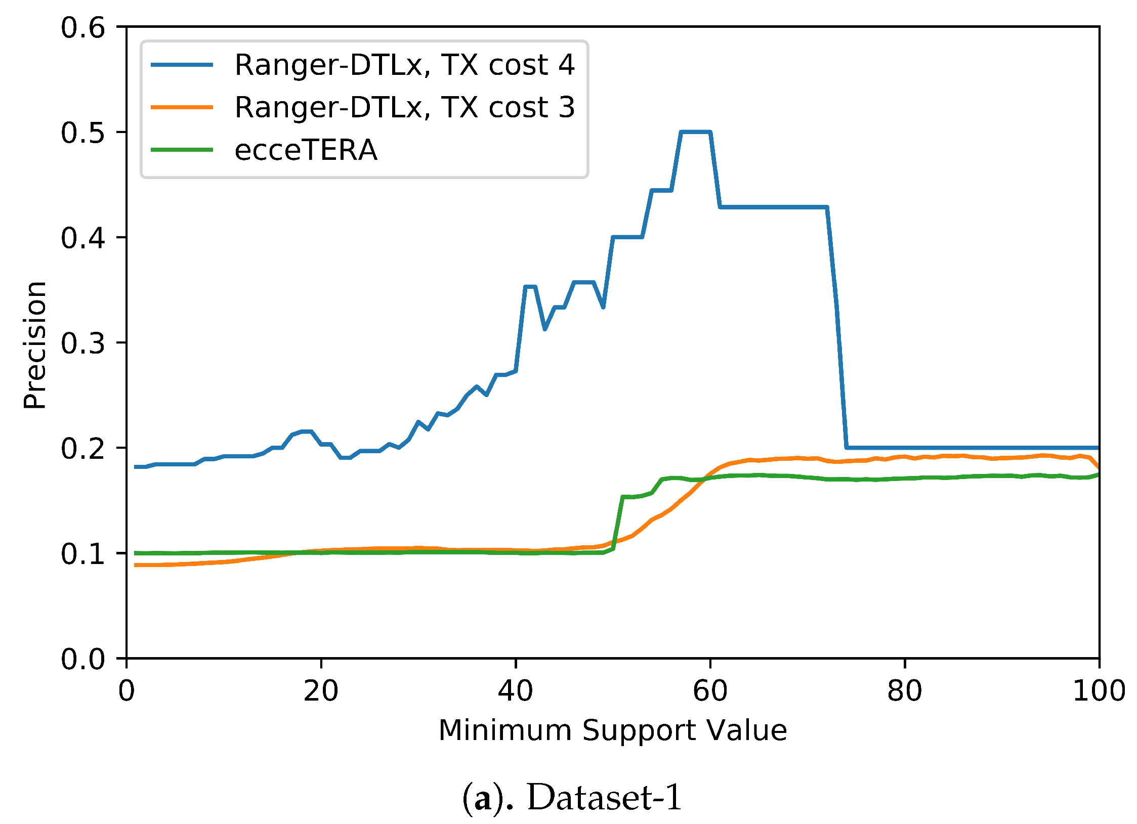
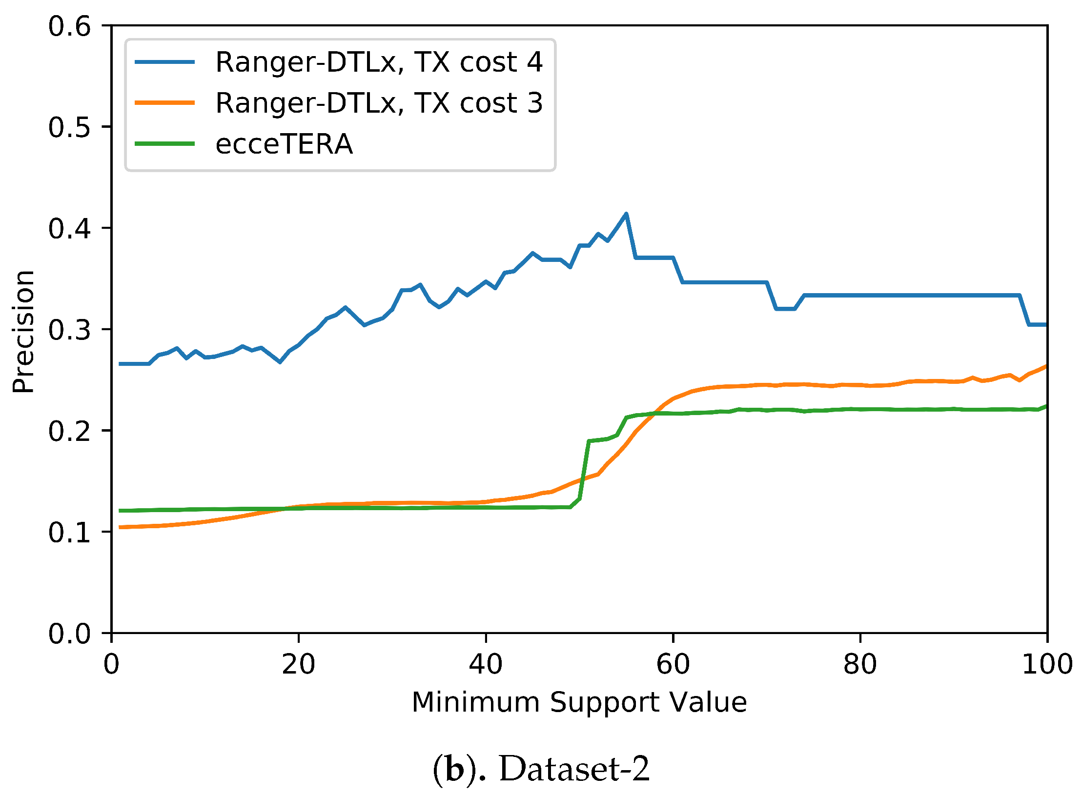
We also assessed if inferred $\mathbb{TX}$ events that have higher support (i.e., are inferred in at least some fraction of all optimal reconciliations for that gene tree) are more likely to be correct (i.e., show higher precision). Figure 5 shows the results of this analysis. These results suggest that higher support values do tend to result in greater precision. More precisely, we find that RANGER-DTLx with $\mathbb{TX}$ cost 3 and ecceTERA both shown similar trends in precision, with precision on Dataset-1 increasing from a low of about 0.1 for all inferred $\mathbb{TX}$ events irrespective of support to a high of about 0.18 if only considering $\mathbb{TX}$ events with 100% support, and precision on Dataset-2 increasing from about 0.1 for all inferred $\mathbb{TX}$ events irrespective of support to a high of approximately 0.25 if only considering $\mathbb{TX}$ events with 100% support. However, as expected, the increase in precision comes at the expense of recall (

Table 4. Number of $\mathbb{TX}$ events inferred by the different methods, along with their precision, are shown for different minimum support value cutoffs. Results are aggregated across all 500 gene tree/species tree pairs in each dataset and presented in the form $a/b$, where b is the total number of distinct $\mathbb{TX}$ events inferred across 100 randomly sampled optimal reconciliations for RANGER-DTLx and across the entire optimal solution space for ecceTERA for each gene tree, and a is the number of these $\mathbb{TX}$ events that are correct.

	Dataset-1			Dataset-2
Support	RANGER-DTLx,${\mathit{P}}_{\mathbb{TX}}=\mathbf{4}$	RANGER-DTLx,${\mathit{P}}_{\mathbb{TX}}=\mathbf{3}$	ecceTERA	RANGER-DTLx,${\mathit{P}}_{\mathbb{TX}}=\mathbf{4}$	RANGER-DTLx,${\mathit{P}}_{\mathbb{TX}}=\mathbf{3}$	ecceTERA
>0	$14/77$	$857/9688$	$926/9285$	$34/128$	$1475/$14,134	$1554/$12,884
≥25%	$12/61$	$818/7869$	$885/8825$	$27/84$	$1416/$11,141	$1511/$12,252
≥50%	$4/10$	$445/4036$	$725/6977$	$13/34$	$874/5807$	$1257/9492$
≥75%	$1/5$	$191/1018$	$242/1427$	$8/24$	$473/1932$	$582/2651$
=100%	$1/5$	$91/503$	$199/1140$	$7/23$	$248/940$	$468/2088$

). For example, on Dataset-2, RANGER-DTLx with $\mathbb{TX}$ cost 3 infers a total of 14,134 distinct $\mathbb{TX}$ events with support $>0$ among 100 optimal reconciliation samples but only 940 of these have 100% support, and the corresponding numbers for ecceTERA are 12,884 and 2088, respectively. Remarkably, as Figure 5 shows, RANGER-DTLx with $\mathbb{TX}$ cost 4 achieves a precision of almost 50% on Dataset-1 and over 40% on Dataset-2 when using a support threshold of about 55%. However, as Table 4 shows, the number of $\mathbb{TX}$ events inferred at that support level by RANGER-DTLx with $\mathbb{TX}$ cost 4 is relatively small. The small number of these events likely explains the drop in precision for RANGER-DTLx with $\mathbb{TX}$ cost 4 as the support threshold in increased past ∼60.

Phylogenetic placement of $\mathbb{TX}$ event donors. Identifying the locations on the species tree of unsampled lineages that served as donors for $\mathbb{TX}$ events can offer important insights regarding major unsampled species lineages and can help to better understand the evolutionary histories of gene families. By design, RANGER-DTLx identifies a specific edge/lineage in the species tree where any given $\mathbb{TX}$ event originates from. However, ecceTERA handles $\mathbb{TX}$ events by introducing a single unsampled branch existing outside of the species tree, which represents all unsampled lineages on the species tree and serves as the donor of all $\mathbb{TX}$ events. This makes it difficult to infer the location of unsampled donor lineages on the species tree using ecceTERA. To assess the accuracy of RANGER-DTLx in identifying/placing the unsampled species donor on the species tree, we used all $\mathbb{TX}$ events (across all 100 samples, regardless of support) inferred by RANGER-DTLx that mapped to the correct recipient species and computed the distance on the species tree between the inferred location of the donor and the actual location of the donor (as given by Zombi). This distance is defined as the number of edges between the inferred donor lineage and the true lineage on the full species tree (including extinct lineages) as simulated by Zombi. As

Table 5. Accuracy of placing unsampled species donors on the species tree. All $\mathbb{TX}$ events inferred by each method, regardless of support, for which the recipient species was identified correctly were used for this analysis. The inferred unsampled donor is considered an exact match if the location of the donor lineage on the species tree is the same as the true location of the donor. Numbers for $\mathbb{TX}$ events considered and exact matches are aggregated across all 500 gene tree/species tree pairs in each dataset. The distance between the inferred and true locations of the donor is defined to be the number of edges between the inferred donor lineage and the true lineage on the full species tree (including extinct lineages) as simulated by Zombi.

	Dataset-1			Dataset-2
	# $\mathbb{TX}$ Considered	Exact Matches	Average Distance	# $\mathbb{TX}$ Considered	Exact Matches	Average Distance
RANGER-DTLx Cost 4	14	3 (21.4%)	1.71	34	13 (38.2%)	2.17
RANGER-DTLx Cost 3	857	473 (55.2%)	1.52	1475	689 (46.7%)	2.03
ecceTERA	926	23 (2.5%)	4.90	1554	36 (2.8%)	6.21

shows, RANGER-DTLx performs remarkably well at inferring the location of the unsampled species donor on the species tree, identifying the exact location for almost half the $\mathbb{TX}$ events when the $\mathbb{TX}$ event cost is 3. Results are worse for RANGER-DTLx with $\mathbb{TX}$ cost 4, but this is likely due to small sample sizes. These results also show that even when the donor lineage is not identified exactly, the inferred placement is often close to the actual placement of the unsampled donor. For completeness, results are also shown for ecceTERA and, as expected, the performance of ecceTERA is much worse than that of RANGER-DTLx, both for exact matches and average distance.

4.2. Biological Data

We also applied RANGER-DTLx to a real biological dataset of over 4500 gene trees from 100 broadly sampled, predominantly microbial, species [5]. Specifically, this dataset consisted of 4547 TreeFix-DTL-corrected gene trees [30] rooted using the OptRoot method implemented in RANGER-DTL 2.0 [17]. We partitioned this dataset into three subsets based on the number of taxa present in the gene trees: less than 50 taxa, between 50–100 taxa, and more than 100 taxa. These subsets represent 76.4% (3474), 16.8% (765), and 6.8% (308) of the total number of gene trees, respectively.

We measured the impact, in practice, of allowing for $\mathbb{TL}$ and $\mathbb{TX}$ events by (i) counting the number of gene trees for which the cost of an optimal reconciliation decreases when $\mathbb{TL}$ and $\mathbb{TX}$ are allowed, and (ii) counting the number of gene trees for which the cost of an optimal reconciliation does not decrease but for which there exist optimal reconciliations that invoke $\mathbb{TL}$ or $\mathbb{TX}$ events. We found that only 28 gene trees showed a reduction in reconciliation cost when reconciled using RANGER-DTLx with a $\mathbb{TX}$ cost of 4 as compared to using RANGER-DTL. This number increases to 76 when a smaller $\mathbb{TX}$ cost of 3 is used. However, as

Table 6. Number of biological dataset gene trees that result in additional co-optimal reconciliations invoking $\mathbb{TL}$ and/or $\mathbb{TX}$ events. These results are based on event costs of 1, 2, 3, 4, and 4, for losses, duplications, transfers, $\mathbb{TL}$, and $\mathbb{TX}$, respectively.

Dataset Size	Total # Gene Trees	Gene Trees with Additional Co-Optimal Solutions
<50 taxa	3474	1350 (38.9%)
50–100 taxa	765	667 (87.2%)
>100 taxa	308	292 (94.8%)

shows, 50.7% of the gene trees, and nearly all of the gene trees with at least 50 leaves, had more optimal reconciliations even when using RANGER-DTLx with the higher $\mathbb{TX}$ cost of 4. This is a result of some (but not all) of the co-optimal reconciliations invoking $\mathbb{TL}$ and/or $\mathbb{TX}$ events. These results suggest that while $\mathbb{TL}$ and $\mathbb{TX}$ events clearly lead to more parsimonious reconciliations in some cases for many gene trees it may be difficult to confidently infer if $\mathbb{TL}$ and $\mathbb{TX}$ events have in fact occurred.

Runtime analysis. We also compared the runtimes of ecceTERA (undated version), RANGER-DTL, and RANGER-DTLx. Average runtimes for these methods on the three subsets of the biological dataset are shown in

Table 7. Runtime comparison on the biological dataset.

Dataset Size	RANGER-DTL	RANGER-DTLx	ecceTERA
<50 leaves	<1 s	$2.5$ s	<1 s
50–100 leaves	<1 s	$12.4$ s	<1 s
>100 leaves	<1 s	$24.5$ s	<1 s

. As the table shoes, RANGER-DTL and ecceTERA are both extremely efficient, averaging a runtime of smaller than 1 s on all three subsets. As expected, given the increased complexity of the model, RANGER-DTLx takes longer than RANGER-DTL and ecceTERA on all three subsets but still remains highly efficient and scalable, averaging just a few seconds on even the subset with the largest gene trees. All timed experiments were run using a single core on a 2.8 GHz × 4 Intel Core i7 processor with 16 GB of RAM.

5. Discussion and Conclusions

In this work, we introduced an extension of the classical DTL reconciliation model, called the DTLx reconciliation model, that accounts for extinct or unsampled species lineages and allows for $\mathbb{TL}$ and $\mathbb{TX}$ events. The resulting method, RANGER-DTLx, handles these additional evolutionary events in a more functional manner compared to ecceERA, the only other parsimony-based model that also handles these events, while matching the time complexity of the fastest known algorithms for DTL reconciliation. Perhaps the most important contribution of this work is our systematic evaluation of the impact of accounting for $\mathbb{TL}$ and $\mathbb{TX}$ events and unsampled lineages on the accuracy of DTL reconciliation and of our ability to correctly detect $\mathbb{TX}$ events. This evaluation, using both simulated and biological data, reveals many new insights that are important for understanding and interpreting microbial gene family evolution and that can inform the development of more sophisticated reconciliation models: First, we find that DTLx reconciliation (i.e., both RANGER-DTLx and ecceTERA) does not noticeably result in improved overall reconciliation accuracy compared to the simpler DTL reconciliation model. Second, we find that there is a very clear tradeoff between the precision and recall of $\mathbb{TX}$ event detection, with precision remaining below 50% for even the most restrictive selection of $\mathbb{TX}$ events and generally staying below 20% for non-negligible values (say, >0.3) of recall. Furthermore, third, our results on the biological dataset indicate that while allowing for $\mathbb{TL}$ and $\mathbb{TX}$ events leads to more parsimonious reconciliations in some cases, for the majority of gene trees $\mathbb{TL}$ and $\mathbb{TX}$ events lead to co-optimal reconciliations that can make it difficult to confidently infer if $\mathbb{TL}$ and $\mathbb{TX}$ events have, in fact, occurred. Nonetheless, we do find that DTLx reconciliation is indeed capable of identifying at least some $\mathbb{TX}$ events with reasonable confidence and that RANGER-DTLx is actually able to find the phylogenetic placement of the unsampled donor of a $\mathbb{TX}$ event with fairly high accuracy.

Our experimental results suggest that it may be possible to use RANGER-DTLx to identify and locate major unsampled lineages on the tree of life and it would be interesting to further explore this application of the new DTLx reconciliation model. Several aspects of the proposed model could also be improved or evaluated further. In particular, though the proposed DTLx reconciliation model uses an undated species tree, the model can be easily extended to work with fully dated species trees. It is possible that the use of dated species trees may help to improve the precision and recall of $\mathbb{TX}$ event inference and this possibility should be explored further. In particular, the use of a dated species tree can help identify transfers that appear to be going forward in time (i.e., where the recipient of a transfer event appears to be more recent than its donor), suggesting the presence of $\mathbb{TX}$ events. Likewise, though RANGER-DTLx allows for the use of distance-dependant transfer costs, we did not evaluate the impact of using this feature in our current study. Using distance-dependent transfer costs (including $\mathbb{TL}$ and $\mathbb{TX}$ costs) may help to improve $\mathbb{TX}$ inference accuracy. Finally, our experimental study suggests that precise detection of $\mathbb{TX}$ events may be difficult to achieve using phylogenetic reconciliation alone, and that additional techniques may be needed to more accurately detect and account for $\mathbb{TX}$ events in microbial gene family evolution.

References

- Tofigh, A. Using Trees to Capture Reticulate Evolution: Lateral Gene Transfers and Cancer Progression. Ph.D. Thesis, KTH Royal Institute of Technology, Stockholm, Sweden, 2009. [Google Scholar]
- Gorbunov, K.Y.; Liubetskii, V.A. Reconstructing genes evolution along a species tree. Molekuliarnaia Biologiia 2009, 43, 946–958. [Google Scholar] [CrossRef] [PubMed]
- Doyon, J.P.; Scornavacca, C.; Gorbunov, K.Y.; Szöllosi, G.J.; Ranwez, V.; Berry, V. An Efficient Algorithm for Gene/Species Trees Parsimonious Reconciliation with Losses, Duplications and Transfers. In Research in Computational Molecular Biology—Comparative Genomics; Tannier, E., Ed.; Springer: Berlin/Heidelberg, Germany, 2010; Volume 6398, pp. 93–108. [Google Scholar]
- Tofigh, A.; Hallett, M.T.; Lagergren, J. Simultaneous Identification of Duplications and Lateral Gene Transfers. IEEE/ACM Trans. Comput. Biol. Bioinform. 2011, 8, 517–535. [Google Scholar] [CrossRef]
- David, L.A.; Alm, E.J. Rapid evolutionary innovation during an Archaean genetic expansion. Nature 2011, 469, 93–96. [Google Scholar] [CrossRef] [Green Version]
- Chen, Z.Z.; Deng, F.; Wang, L. Simultaneous Identification of Duplications, Losses, and Lateral Gene Transfers. IEEE/ACM Trans. Comput. Biol. Bioinform. 2012, 9, 1515–1528. [Google Scholar] [CrossRef] [Green Version]
- Bansal, M.S.; Alm, E.J.; Kellis, M. Efficient algorithms for the reconciliation problem with gene duplication, horizontal transfer and loss. Bioinformatics 2012, 28, 283–291. [Google Scholar] [CrossRef]
- Stolzer, M.; Lai, H.; Xu, M.; Sathaye, D.; Vernot, B.; Durand, D. Inferring duplications, losses, transfers and incomplete lineage sorting with nonbinary species trees. Bioinformatics 2012, 28, 409–415. [Google Scholar] [CrossRef] [Green Version]
- Szollosi, G.J.; Boussau, B.; Abby, S.S.; Tannier, E.; Daubin, V. Phylogenetic modeling of lateral gene transfer reconstructs the pattern and relative timing of speciations. Proc. Natl. Acad. Sci. USA 2012, 109, 17513–17518. [Google Scholar] [CrossRef] [Green Version]
- Szollosi, G.J.; Tannier, E.; Lartillot, N.; Daubin, V. Lateral Gene Transfer from the Dead. Syst. Biol. 2013, 62, 386–397. [Google Scholar] [CrossRef]
- Bansal, M.S.; Alm, E.J.; Kellis, M. Reconciliation Revisited: Handling Multiple Optima when Reconciling with Duplication, Transfer, and Loss. J. Comput. Biol. 2013, 20, 738–754. [Google Scholar] [CrossRef] [PubMed] [Green Version]
- Scornavacca, C.; Paprotny, W.; Berry, V.; Ranwez, V. Representing a Set of Reconciliations in a Compact Way. J. Bioinform. Comput. Biol. 2013, 11, 1250025. [Google Scholar] [CrossRef] [PubMed] [Green Version]
- Libeskind-Hadas, R.; Wu, Y.C.; Bansal, M.S.; Kellis, M. Pareto-optimal phylogenetic tree reconciliation. Bioinformatics 2014, 30, i87–i95. [Google Scholar] [CrossRef] [PubMed] [Green Version]
- Sjostrand, J.; Tofigh, A.; Daubin, V.; Arvestad, L.; Sennblad, B.; Lagergren, J. A Bayesian Method for Analyzing Lateral Gene Transfer. Syst. Biol. 2014, 63, 409–420. [Google Scholar] [CrossRef] [Green Version]
- Scornavacca, C.; Jacox, E.; Szöllosi, G.J. Joint amalgamation of most parsimonious reconciled gene trees. Bioinformatics 2015, 31, 841–848. [Google Scholar] [CrossRef] [Green Version]
- Jacox, E.; Chauve, C.; Szollosi, G.J.; Ponty, Y.; Scornavacca, C. ecceTERA: Comprehensive gene tree-species tree reconciliation using parsimony. Bioinformatics 2016, 32, 2056. [Google Scholar] [CrossRef]
- Bansal, M.S.; Kellis, M.; Kordi, M.; Kundu, S. RANGER-DTL 2.0: Rigorous reconstruction of gene-family evolution by duplication, transfer and loss. Bioinformatics 2018, 34, 3214–3216. [Google Scholar] [CrossRef]
- Kordi, M.; Bansal, M.S. Exact Algorithms for Duplication-Transfer-Loss Reconciliation with Non-Binary Gene Trees. IEEE/ACM Trans. Comput. Biol. Bioinform. 2019, 16, 1077–1090. [Google Scholar] [CrossRef]
- Merkle, D.; Middendorf, M.; Wieseke, N. A parameter-adaptive dynamic programming approach for inferring cophylogenies. BMC Bioinform. 2010, 11, S60. [Google Scholar] [CrossRef] [PubMed] [Green Version]
- Conow, C.; Fielder, D.; Ovadia, Y.; Libeskind-Hadas, R. Jane: A new tool for the cophylogeny reconstruction problem. Algorithms Mol. Biol. 2010, 5, 16. [Google Scholar] [CrossRef] [PubMed] [Green Version]
- Donati, B.; Baudet, C.; Sinaimeri, B.; Crescenzi, P.; Sagot, M.F. EUCALYPT: Efficient tree reconciliation enumerator. Algorithms Mol. Biol. 2015, 10, 3. [Google Scholar] [CrossRef] [PubMed] [Green Version]
- Santichaivekin, S.; Yang, Q.; Liu, J.; Mawhorter, R.; Jiang, J.; Wesley, T.; Wu, Y.C.; Libeskind-Hadas, R. eMPRess: A systematic cophylogeny reconciliation tool. Bioinformatics 2020, btaa978. [Google Scholar] [CrossRef] [PubMed]
- Williams, D.; Gogarten, J.P.; Papke, R.T. Quantifying Homologous Replacement of Loci between Haloarchaeal Species. Genome Biol. Evol. 2012, 4, 1223–1244. [Google Scholar] [CrossRef] [Green Version]
- Ovadia, Y.; Fielder, D.; Conow, C.; Libeskind-Hadas, R. The Cophylogeny Reconstruction Problem Is NP-Complete. J. Comput. Biol. 2011, 18, 59–65. [Google Scholar] [CrossRef]
- Libeskind-Hadas, R.; Charleston, M. On the Computational Complexity of the Reticulate Cophylogeny Reconstruction Problem. J. Comput. Biol. 2009, 16, 105–117. [Google Scholar] [CrossRef]
- Hasić, D.; Tannier, E. Gene tree reconciliation including transfers with replacement is NP-hard and FPT. J. Comb. Optim. 2019, 38, 502–544. [Google Scholar] [CrossRef] [Green Version]
- Kordi, M.; Kundu, S.; Bansal, M.S. On Inferring Additive and Replacing Horizontal Gene Transfers Through Phylogenetic Reconciliation. In Proceedings of the 10th ACM International Conference on Bioinformatics, Computational Biology and Health Informatics, Niagara Falls, NY, USA, 7–10 September 2019; pp. 514–523. [Google Scholar] [CrossRef] [Green Version]
- Zhaxybayeva, O.; Gogarten, J.P. Horizontal gene transfer, gene histories, and the root of the tree of life. In Planetary Systems and the Origins of Life; Pudritz, R., Higgs, P., Stone, J., Eds.; Cambridge Astrobiology; Cambridge University Press: Cambridge, UK, 2007; pp. 178–192. [Google Scholar] [CrossRef]
- Davín, A.A.; Tricou, T.; Tannier, E.; de Vienne, D.N.; Szollosi, G.J. Zombi: A phylogenetic simulator of trees, genomes and sequences that accounts for dead linages. Bioinformatics 2019, 36, 1286–1288. [Google Scholar] [CrossRef] [PubMed]
- Bansal, M.S.; Wu, Y.C.; Alm, E.J.; Kellis, M. Improved gene tree error correction in the presence of horizontal gene transfer. Bioinformatics 2015, 31, 1211–1218. [Google Scholar] [CrossRef] [PubMed] [Green Version]
Figure 1.
Illustration of the difference between (a) a standard transfer event and (b) a event.
Figure 2.
An example gene tree (a) and a possible augmented version with hidden nodes in blue (b).
Figure 3.
Representation of unsampled lineages on the species tree. (a) Illustration of the “coral” of life based on drawings by Darwin, where black lines represent lineages leading to extant species, and grey lines represent potential unsampled species; adapted from [28]. (b) Input species tree before augmentation. (c) Augmented species tree. Extra nodes are in green and extra leaves are in white. Leaves labeled A-D represent extant species. Unsampled lineages are represented by the edges connecting extra nodes and extra leaves.
Figure 4.
Impact of and events on optimal DTLx reconciliations. (a) and (b) are the input gene tree and input species tree , respectively. (c) An augmented version of containing a single hidden node as required by the reconciliations shown in Parts (e,f). (d) An optimal DTL reconciliation of and illustrating how the gene tree (blue lines) may have evolved within the species tree (tubes) without the use of or events. This DTL reconciliation invokes two transfer events and two losses. All reconciliations shown in this figure use event costs of 1, 2, 3, 4, and 3 for losses, duplications, transfers, , and events, respectively. Thus, we get a total reconciliation cost of 8 for this optimal DTL reconciliation. (e) An optimal reconciliation of G and S that uses events but not events. This reconciliation utilizes the hidden node h1 in to facilitate a event from species E to species B. It invokes one transfer event and one event, for a total reconciliation cost of 7. (f) An optimal DTLx reconciliation of G and S. This DTLx reconciliation utilizes the hidden node h1 in to facilitate a event. It invokes one transfer event and one event, for a total reconciliation cost of 6. Accordingly, the reconciliation shown in (f) makes use of an extra leaf and extra node on (dotted green tube).
Figure 5.
Impact of increasing support values on event accuracy. The support for an event is defined as the percentage of optimal solution space that the event appears in.