Adaptive Self-Scaling Brain-Storm Optimization via a Chaotic Search Mechanism

Abstract

Brain-storm optimization (BSO), which is a population-based optimization algorithm, exhibits a poor search performance, premature convergence, and a high probability of falling into local optima. To address these problems, we developed the adaptive mechanism-based BSO (ABSO) algorithm based on the chaotic local search in this study. The adjustment of the search space using the local search method based on an adaptive self-scaling mechanism balances the global search and local development performance of the ABSO algorithm, effectively preventing the algorithm from falling into local optima and improving its convergence accuracy. To verify the stability and effectiveness of the proposed ABSO algorithm, the performance was tested using 29 benchmark test functions, and the mean and standard deviation were compared with those of five other optimization algorithms. The results showed that ABSO outperforms the other algorithms in terms of stability and convergence accuracy. In addition, the performance of ABSO was further verified through a nonparametric statistical test.

1. Introduction

Meta-heuristic algorithms have attracted increasing attention in recent years due to their unique advantages in solving high-dimensional and complex optimization problems and have been successfully applied to communication, transportation, national defense, management and computer science [1,2,3,4,5]. Deterministic algorithms usually start from a similar initial point and obtain the same solution in the iterative process, but the search process can easily fall into local optima. The development of meta-heuristic algorithms has accelerated in the past few decades. These algorithms use random operators to start with random initialization, which can avoid local optima [6]. In addition to randomness, meta-heuristic algorithms can handle approximation and uncertainty and adapt to problems. These characteristics ensure that meta-heuristic algorithms can be developed freely for a variety of classifications. Several optimization algorithms have been created based on biological populations or population mechanisms, e.g., the differential evolution (DE) algorithm [7,8,9], particle swarm optimization (PSO) algorithm [10,11,12], gravitational search algorithm (GSA) [13,14,15], whale optimization algorithm (WOA) [16,17,18] and artificial bee colony (ABC) algorithm [19,20]. All these variants have achieved great success in solving practical problems in many fields such as artificial neural network learning [21,22,23,24], protein structure prediction [25,26,27], time series prediction [28,29,30], and dendritic neuron learning [31,32]. Brain-storm optimization (BSO) is a swarm intelligence algorithm with broad application prospects in solving complicated problems [33,34,35]. BSO is inspired by human brainstorming, in which every thought produced by the human brain represents an individual in the search space. During brainstorming, people first generate rough ideas and then exchange and discuss these ideas with others, during which low-level ideas are eliminated and great ones are retained. The brainstorming process is repeated, and the ideas become increasingly mature. New ideas are constantly generated and added to the final list. Once the process is finished, a feasible and effective idea is presented.

Since it was proposed in 2011, BSO has been a focus of swarm intelligence research due to its novelty and efficiency. BSO has been successfully applied to various scenarios such as function optimization, engineering optimization, and financial prediction [4,36,37,38,39]. However, as with other swarm intelligence optimization algorithms, BSO is prone to falling into local optima and premature convergence. Many variants have been proposed to improve various aspects of the performance of BSO. For example, the chaotic brain-storm optimization (CBSO) algorithm proposed by Yu et al. effectively improves the search performance of BSO [40]. Because it does not use an adaptive strategy, the algorithm is not ideal when dealing with complex functions. For swarm intelligence optimization algorithms, the balance between convergence and divergence is of great significance; premature convergence leads to a low population diversity and poor-quality solutions, while overmature convergence results in very slow search speeds. In references [40,41], chaotic sequences were used as variables to initialize the population and to generate new individuals. Chaos, as a universal phenomenon of nonlinear dynamic systems, is unpredictable and non-repetitive. Hence, its randomicity and ergodicity can effectively improve the population diversity and solution quality of BSO. Reference [42] used 12 chaotic maps to generate chaotic variables for the chaotic local search (CLS) process and embedded this process into their algorithm according to different schemes; in addition, a multiple chaos embedded chaotic parallel gravitational search algorithm (CGSA-P) was proposed. However, during iteration, the individuals converged rapidly, and it was difficult to adjust the search range. Therefore, simply replacing random variables with chaotic variables cannot effectively improve the search performance of the algorithm. To overcome the limitations of the CLS, we developed an adaptive self-scaling mechanism to control the search range of the CLS and embedded the improved CLS into BSO (referred to as adaptive mechanism-based BSO, ABSO). The proposed ABSO algorithm was then expanded into two types of algorithms, i.e., chaotic sequence random selection (ABSO-R) and chaotic sequence parallel search (ABSO-P) algorithms. Then, random selection and parallel computing were carried out on the 12 chaotic maps. During the optimization process, as the position of the population changes, the CLS search region is determined by the positions of 2 random individuals in the entire search space. After each iteration, the adaptive machine carries out the CLS process, therefore improving the search performance and convergence speed of the algorithm. To verify the performance of the proposed algorithm, we used 29 benchmark functions from IEEE CEC 2017 and compared the results of the proposed algorithm with those of five other algorithms, i.e., BSO, CBSO, CGSA-P, DE and WOA. Furthermore, we verified the effectiveness and superiority of ABSO using the Friedman nonparametric statistical test [43,44]. The simulation and verification results showed that ABSO is strongly competitive in terms of its search accuracy, convergence speed, and stability. The main contributions of this study are as follows:

• An improved adaptive CLS strategy is proposed to enhance the global search performance of BSO.
• Adaptive scaling CLS can effectively help BSO jump out of local optima and avoid premature convergence of the BSO algorithm.
• Extensive experimental results show that ABSO is superior to its competitors.
• The results of two nonparametric statistical tests indicate that the proposed adaptive self-scaling mechanism effectively improves the search ability and efficiency of ABSO.

The remainder of this paper is organized as follows: Section 2 presents a brief description of the classic BSO algorithm. Section 3 introduces 12 different chaotic maps and the parameters. Section 4 describes the CLS method based on adaptive self-scaling and its integration with BSO. Section 5 presents the experimental and statistical analysis results. Section 6 concludes this study and presents future research work.

2. Brain-Storm Optimization

BSO is a swarm intelligence algorithm inspired by human brainstorming. During the search process, it abstracts individuals into ideas generated by the human brain, and the solution set of the optimization problem is assumed to be a group of individuals in the solution space. During the execution of the algorithm, BSO ensures the diversity of individuals and the convergence speed of the algorithm using three main operations: clustering, selecting, and generating individuals. In the first step of clustering, individuals are gathered to discuss and share their different ideas or viewpoints. For a given problem, the clustering results reflect the distribution of individuals in the search space. The k-means clustering method is the classic BSO algorithm for dividing individuals in a population into several clusters according to the distance between individuals. With the iteration of the clustering method, the distribution of individuals moves to an increasingly smaller range, which reduces the number of redundant and similar solutions. In the second step of selection, relatively optimized individuals are selected for the next iteration. BSO controls the selection process by setting some parameters [42]. To maintain the diversity of the population, a random replacement scheme is used for the original population, and the probability pc determines if the cluster center is replaced by randomly generated individuals. After selection, the final step is to generate individuals. In this stage, a candidate solution set is generated based on a new idea. Mutation individuals are generated using the following equation:

$$Z_{\mathrm{new}}^i=Z^i+\mu ·M(0,1),$$

(1)

where $Z^i$ and $Z_{new}^i$ denote the new individuals that are selected and generated in the i-th dimension, respectively; $M(0,1)$ is a random variable with a standard Gaussian distribution; and $\mu$ stands for the step value, which changes with the interaction between individuals during the iteration and can be calculated based on the following equation:

$$\mu =logsig\left(\frac{{Max}_i\times 0.5-Cu{r}_i}{N}\right)·rand(0,1),$$

(2)

where $logsig\left(\right)$ is the log-sigmoid transfer function within the interval (0,1); $Ma{x}_i$ and $Cu{r}_i$ denote the maximum number of iterations and the current number of iterations, respectively; N is a positive number, commonly in the range of [0.3, 0.6], that is designed to control the change rate of the $logsig\left(\right)$ function; and rand() ensures that the range of $\mu$ is (0, 1) and changes adaptively with the number of iterations. The combination of this parameter and Cauchy mutation is conducive to the early exploration and later exploitation of the algorithm. If the newly generated individual is superior to the current individual, the current individual is replaced by the new individual. Once the replacement is completed, the algorithm enters the next iteration. The classic BSO algorithm is an optimization algorithm based on the iterative process that iteratively generates the solution to a problem using the above three operations until the predefined conditions of terminating the iteration are satisfied.

3. Chaotic Maps

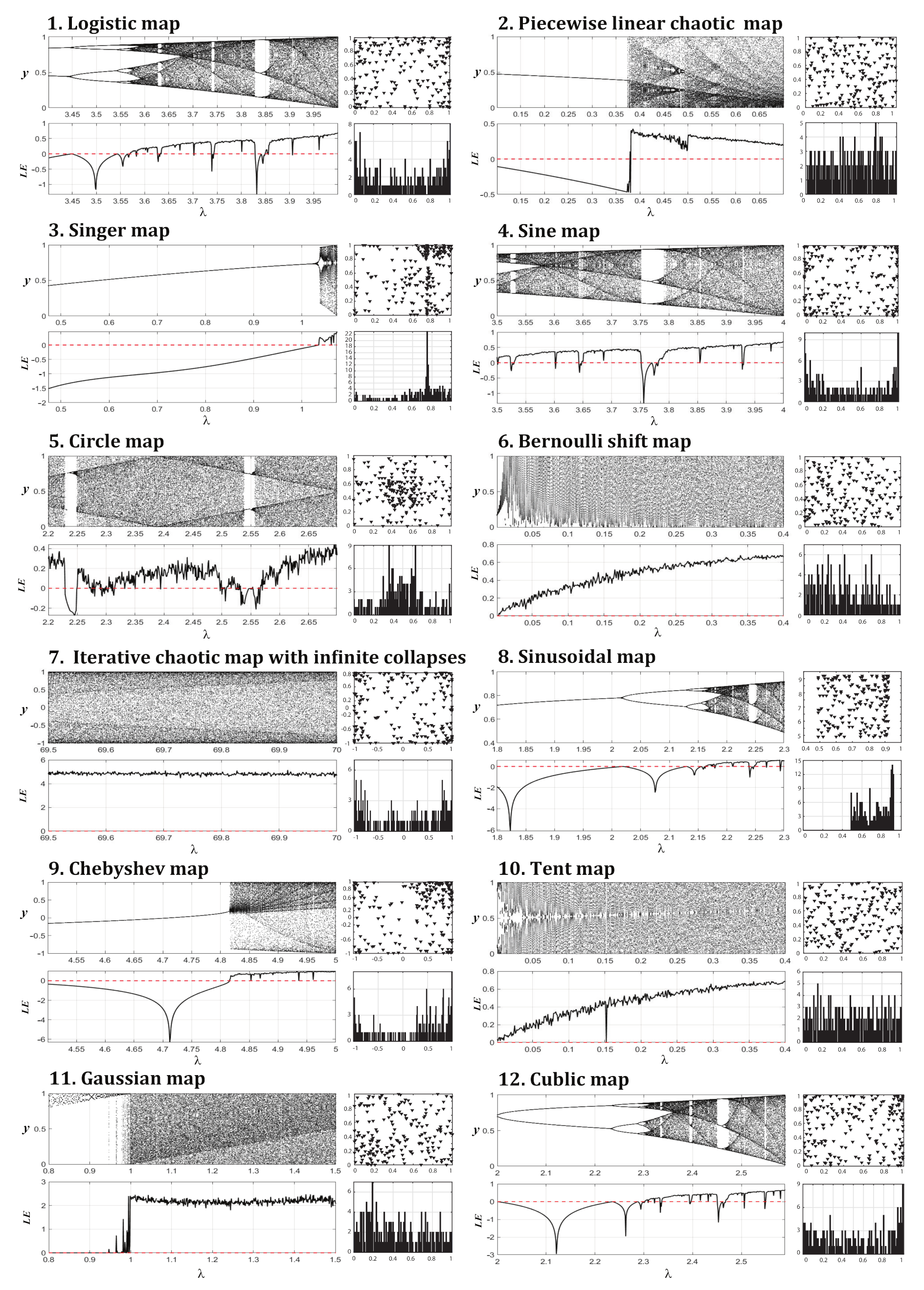
One-dimensional irreversible mapping is the simplest system capable of producing chaotic motion. The chaotic sequences produced by different chaotic maps, as well as their distributions and ergodic properties, are completely different. Due to the ergodicity and non-repetition of chaotic sequences, searches with various chaotic maps outperform searches with a single chaotic map in terms of both the search range and the accuracy. Chaotic maps are used to generate chaotic sequences that are then implemented in the CLS strategy. In this study, 12 one-dimensional chaotic maps were selected to form chaotic mutation operators to constitute the search strategies, which effectively prevented the algorithm from falling into local optima. The 12 chaotic maps are briefly described as follows:

• A logistic map is a classic chaotic map in the nonlinear dynamics of a biological population that can be expressed as follows:

  $$y_{n+1}=\beta y_n\left(1-y_n\right),$$

  (3)

  where $y_n$ denotes the n-th chaotic sequence and $y_n\in (0,1)$, $y_0\notin \{0,0.25,0.5,0.75,1\}$. In this study, we set $\beta =4$, and the initial chaotic value was $y_0=0.152$.
• A piecewise linear chaotic map (PWLCM) has a constant density function in the defined interval. The simplest PWLCM can be obtained by the following equation:

  $$y_{n+1}=\left\{\begin{array}{cc}{y}_n/\beta ,& y_n\in (0,\beta )\\ \left(1-y_n\right)(1-\beta ),& y_n\in [\beta ,1)\end{array}\right.$$

  (4)
  In our experiment, the initial chaotic sequence was $y_0=0.002$, and we set $\beta =0.7$.
• A Singer map is similar to a one-dimensional chaotic system:

  $$y_{n+1}=\beta \left(7.86y_n-23.31y_n^2+28.75y_n^3-13.302875y_n^4\right),$$

  (5)

  when the Singer map shows chaotic behavior, parameter $\beta \in (0.9,1.08)$. In this study, we set $y_0=0.152$ and $\beta =1.073$.
• A sine map is similar to a unimodal logistic map and can be expressed by the following formula:

  $$y_{n+1}=\frac{\beta }{4}sin\left(\pi y_n\right),$$

  (6)

  where $\beta \in (0,4]$, $y_0\in (0,1)$, and we determined that $\beta =4$ and $y_0=0.152$.
• A circle map is a simplified one-dimensional model for driven mechanical rotors and phase locked loops in electronics that maps a circle onto itself and can be expressed by the following equation:

  $$y_{n+1}=y_n+\alpha -\frac{\beta }{2\pi }sin\left(2\pi y_n\right)mod\left(1\right),$$

  (7)

  when $\alpha =0.5$ and $\beta =2.2$, the chaotic sequences within the interval of (0,1) can be obtained based on the above equation. The initial value was set to $y_0=0.152$.
• A Bernoulli shift map is a type of piecewise linear map that is similar to a tent map and can be expressed as follows:

  $$y_{n+1}=\left\{\begin{array}{cc}{y}_n/(1-\beta ),& 0<y_n\le 1-\beta \\ \left(y_n-1+\beta \right)/\beta ,& 1-\beta <y_n<1\end{array}\right.$$

  (8)
  In this study, we set $\beta =0.4$ and $y_0=0.152$.
• An iterative chaotic map with infinite collapses (ICMIC) obtains infinite fixed points based on the following equation:

  $$y_{n+1}=sin\frac{b}{y_n},$$

  (9)

  where the adjustable parameter $b\in (0,+\infty )$. In this study, $b=70$. Therefore, the chaotic sequences are in (−1, 1), and $y_n\ne 0$; if the generated sequence is negative, the absolute value is taken.
• A sinusoidal map can be generated by the following formula:

  $$y_{n+1}=b{y}_n^{2}sin\left(\pi y_n\right),$$

  (10)

  where $y_0=0.74$, and $b=2.3$.
• Chebyshev maps are widely used in digital communication, neural computing and safety maintenance. The process to generate chaotic sequences is defined as follows:

  $$y_{n+1}=cos\left(\rho ·{cos}^{-1}{y}_n\right),$$

  (11)

  where $\rho =5$, and $y_0=0.152$.
• A topological conjugacy relationship exists between the famous logistic map and the tent map, so the two are interconvertible. Tent map sequences can be calculated by the following formula:

  $$y_{n+1}=\left\{\begin{array}{cc}{y}_n/\beta ,& 0<y_n\le \beta \\ \left(1-y_n\right)/(1-\beta ),& \beta <y_n\le 1\end{array}\right.$$

  (12)

  where $\beta =4$, and $y_0=0.152$.
• A Gaussian map can be generated by the following formula:

  $$y_{n+1}=\left\{\begin{array}{cc}0,& y_n=0\\ \left(\rho /y_n\right)mod\left(1\right),& y_n\ne 0\end{array}\right.$$

  (13)
• Cubic maps are usually used in cryptography, and the sequence calculation formula is as follows:

  $$y_{n+1}=\rho ·y_n\left(1-y_n^2\right),$$

  (14)
  We set $y_0=0.152$ and $\rho =2.59$ in our experiment.

Figure 1 shows the sequence distribution graph of the 12 chaotic maps after ${10}^3$ iterations. Different chaotic maps show different distributions. The Lyapunov exponent (LE) is an index used to determine if a system has chaotic characteristics. As shown in Figure 1, when chaotic characteristics occur, the value of $\lambda$ in the corresponding Lyapunov function should ensure that the LE value is positive. Hence, in the experiment, we set the parameter values and initial values for the chaotic maps according to these characteristics.

4. CLS Based on Adaptive Self-Scaling

Chaos, as a characteristic of nonlinear dynamic systems, is characterized by boundedness, dynamic instability, pseudo-randomness, ergodicity, and aperiodicity and depends on the initial value and control parameters. Because of the ergodicity and randomicity, the chaotic system changes randomly. If the time period is long enough, the chaotic system eventually experiences every single state. Based on this characteristic, chaotic systems can be used to establish a search operator for optimizing the objective function. Though chaotic optimization works well in small search spaces, the optimization time in large search spaces is unacceptable [45]. Hence, chaotic searches are often integrated into other global optimization algorithms, e.g., the evolutionary algorithm, to improve their search ability. By substituting random sequences of control parameters into BSO, the above 12 chaotic maps can generate chaotic sequences in the local search process. In a study by our group [40], the local search strategy was proven to be an effective method to improve the search ability of BSO. However, traditional algorithms are likely to fall into local optima. Thus, we used the adaptive self-scaling mechanism to further improve the search ability of the BSO algorithm. The CLS with a single chaotic map is defined as follows:

$$Z_b^t=Z_c^t+radius\left(t\right)·(U-L)*\left(y_t-0.5\right),$$

(15)

where $Z_c^t$ represents the position where the algorithm obtains the current optimal solution during the t-th iteration; $Z_b^t$ denotes the position of the new individual generated from the current optimal solution through the CLS strategy; U and L stand for the upper and lower bounds of the search space, respectively, where $y_t$ is a chaotic variable gained based on one of the 12 chaotic maps; and $radius\left(t\right)$ refers to the chaotic search radius to control the search range, with $radius\left(t\right)\in (0,1)$. The radius gradually decreases as the number of iterations increases, and the radius variation is defined as follows:

$$radius(t+1)=\gamma ·radius\left(t\right),$$

(16)

where $\gamma$ is an adjustable coefficient that was set to 0.986 in this study, and the initial search radius $radius\left(0\right)=0.03$.

According to its definition, the CLS strategy is decided by the search radius. However, applying the same search radius scaling scheme for different optimization problems is not ideal. We developed an adaptive chaotic search strategy for different problems, in which the search range can be adaptively scaled:

$$Z_b^t=Z_c^t+\left|Z_i^t-Z_j^t\right|·\left(y_t-0.5\right),$$

(17)

where $Z_i^t$ and $Z_j^t$ are two randomly selected individuals from the current population; that is, in each CLS process, the search range changes with the position of the current population. In the entire search process, if the new solution obtained by the improved CLS scheme outperforms the current optimal individual in terms of fitness, it replaces the current optimal individual. Otherwise, the current individual is kept until the next iteration. Thus, a single update operation can be performed according to the following formula:

$$Z_c^{t+1}=\left\{\begin{array}{cc}{Z}_b^t,& \mathrm{if}Fit\left(Z_b^t\right)\le Fit\left(Z_c^t\right)\\ Z_c^t,& \mathrm{otherwise}.\end{array}\right.$$

(18)

Based on the analysis and existing improvements in the BSO algorithm, we developed ABSO, which improves the search performance of the algorithm by adaptively adjusting the CLS radius. The specific steps of Algorithm 1 are as follows:

Algorithm 1: ABSO

01: for all Randomly generate a population with N individuals and calculate the fitness of each individual. do

02: Divide N individuals into Mclusters using the k-means method; the optimal individual in each cluster is

chosen as the center.

03: Select the cluster center:

04: if $rand(0,1)<p=0.2$, replace the cluster center with a randomly generated one;

05: if $rand(0,1)<p=0.4$, choose a center based on the current probability, or choose a randomly selected

individual as the center.

06: if $rand(0,1)<p=0.5$ and Steps 04 and 05 are not implemented, choose 2 cluster centers, and combine

them into a new cluster center, or randomly choose 2 individuals to generate a new cluster center.

end-for

07: ABSO-R: Randomly select a mapping function from the 12 chaotic maps, wherein the probability of each

chaotic map being selected is equal.

ABSO-P: The above 12 chaotic maps are selected in parallel.

08: Calculate the chaotic variables according to the selected chaotic mapping Equations (3)–(14).

09: Implement the CLS using the chaotic variables and adaptive self-scaling strategy.

10: Compare the fitness of the current individual with the fitness before the chaotic search based on Equation (18),

update the individual fitness, and output the optimal fitness value.

11: end-all

In the experiment, we extended ABSO into two algorithms, ABSO-R and ABSO-P. In ABSO-R, we randomly selected one of the 12 chaotic map to perform the chaotic search. The probability of each chaotic system being selected is the same, and the chaotic search is defined as follows:

$$Z_b^t=Z_c^t+\left|Z_i^t-Z_j^t\right|·\left(y_{\mathrm{random}}^t-0.5\right),$$

(19)

where $y_{random}^t$ denotes the chaotic variable generated by the selected chaotic sequence. In ABSO-P, the 12 chaotic sequences were calculated in parallel, and the result was compared with the current candidate solution. The execution formula is as follows:

$$Z_b^t=Z_c^t+\left|Z_i^t-Z_j^t\right|·\left(y_m^t-0.5\right),m\in \{1,2,\dots ,12\},$$

(20)

$$Z_b^{t+1}=\left\{\begin{array}{cc}{Z}_b^{t-min},& \mathrm{if}Fit\left(Z_b^{t-min}\right)\le Fit\left(Z_b^t\right)\\ Z_b^t,& \mathrm{otherwise}\end{array}\right.$$

(21)

where $y_m^t$ denotes the 12 chaotic variables, $Z_b^{t-min}$ represents the optimal solution of the 12 parallel candidate solutions, Equation (20) performs the 12 chaotic searches in parallel, and Equation (21) compares and updates the 12 current candidate solutions to ensure the optimal performance of the algorithm.

5. Experimental Studies

In the experiment, the population size of all algorithms was set to $N=100$, the number of dimensions was $D=30$, and the number of iterations was 30. To ensure the fairness of the comparison, the maximum number of iterations was replaced with the maximum number of function evaluations, which was set to $D*5000$. The experimental environment was a $Win1064$ bit system with a 3.80 GHz i7-10770k CPU and 32 GB memory, and the simulation software was MATLAB R2018a.

5.1. Benchmark Functions

To verify the effectiveness of ABSO, all 29 benchmark functions from IEEE CEC 2017 were used in this study. All these functions are for minimization. For example, F1 and F3 are unimodal functions that are usually used to evaluate the convergence speed of algorithms, and F4–F10 are multimodal functions that evaluate the ability of algorithms to jump out of locally optimal solutions. There are also mixed functions (F11–F20) and composite functions (F21–F30), which are often used to test the search ability of algorithms. These functions not only contain a large number of locally optimal solutions but also have a complex search space. Due to its instability in MATLAB, F2 was not included in this study.

5.2. Experimental Results and Analysis

In this study, we compared the proposed algorithm with five other algorithms: BSO, CBSO, CGSA-P, DE and WOA. The parameters of these algorithms were set according to the optimal parameters provided in previous studies. To ensure the fairness of the comparison, we used the number of function evaluations rather than the number of iterations as the termination condition for each algorithm such that each algorithm paid the same calculation cost. The number of function evaluations was 5000, and the population size of all algorithms was 50. Thirty repeated experiments were performed for each algorithm on each test function, and then the results of 30 experiments were compared in terms of the $mean$ and $standarddeviation$. The results are shown in

Table 1. Experimental results of CEC 17 benchmark functions.

	F1	F3	F4	F5	F6
Algorithm	Mean ± Std	Mean ± Std	Mean ± Std	Mean ± Std	Mean ± Std
BSO	2.39$\times {10}^3$± 2.42$\times {10}^2$	6.45$\times {10}^3$± 3.11$\times {10}^2$	5.55$\times {10}^2$± 4.65$\times {10}^1$	7.87$\times {10}^2$± 3.87$\times {10}^1$	6.59$\times {10}^2$± 5.02
CBSO	2.57$\times {10}^3$± 2.44$\times {10}^2$	3.59$\times {10}^2$± 2.11$\times {10}^1$	5.09$\times {10}^2$± 3.55$\times {10}^1$	7.04$\times {10}^2$± 4.00$\times {10}^1$	7.01$\times {10}^2$± 6.53
CGSA-P	1.99$\times {10}^3$± 8.91$\times {10}^2$	7.64$\times {10}^4$± 5.88$\times {10}^3$	4.91$\times {10}^2$± 2.01$\times {10}^1$	7.25$\times {10}^2$± 2.11$\times {10}^1$	6.49$\times {10}^2$± 3.95
DE	2.41$\times {10}^7$± 5.16$\times {10}^6$	7.99$\times {10}^4$± 2.06$\times {10}^4$	5.97$\times {10}^2$± 3.19$\times {10}^1$	7.05$\times {10}^2$± 2.14$\times {10}^1$	6.13$\times {10}^2$± 3.99
WOA	1.51$\times {10}^6$± 2.16$\times {10}^5$	1.47$\times {10}^5$± 7.44$\times {10}^4$	5.66$\times {10}^2$± 2.91$\times {10}^1$	7.26$\times {10}^2$± 6.55$\times {10}^1$	6.71$\times {10}^2$± 1.32
ABSO-R	1.97$\times {10}^3$± 1.71$\times {10}^2$	5.77$\times {10}^3$± 9.34$\times {10}^2$	6.02$\times {10}^2$± 1.11$\times {10}^1$	7.62$\times {10}^2$± 5.91$\times {10}^1$	6.55$\times {10}^2$± 2.54
ABSO-P	2.18$\times {10}^3$± 5.14$\times {10}^2$	3.47$\times {10}^2$± 2.92$\times {10}^2$	4.57$\times {10}^2$± 1.86$\times {10}^1$	6.44$\times {10}^2$± 2.62$\times {10}^1$	6.33$\times {10}^2$± 3.59
	F7	F8	F9	F10	F11
Algorithm	Mean±Std	Mean±Std	Mean±Std	Mean±Std	Mean±Std
BSO	1.59$\times {10}^3$± 8.91$\times {10}^1$	1.09$\times {10}^3$± 3.99$\times {10}^1$	1.09$\times {10}^4$± 2.29$\times {10}^3$	7.95$\times {10}^3$± 6.77$\times {10}^2$	1.45$\times {10}^3$± 4.31$\times {10}^1$
CBSO	1.45$\times {10}^3$± 9.44$\times {10}^1$	8.99$\times {10}^2$± 2.89$\times {10}^1$	5.01$\times {10}^3$± 6.99$\times {10}^2$	5.71$\times {10}^3$± 6.21$\times {10}^2$	1.41$\times {10}^3$± 4.01$\times {10}^1$
CGSA-P	8.88$\times {10}^2$± 1.92$\times {10}^1$	9.41$\times {10}^2$± 2.12$\times {10}^1$	3.03$\times {10}^3$± 5.87$\times {10}^2$	5.97$\times {10}^3$± 3.59$\times {10}^2$	1.51$\times {10}^3$± 6.99$\times {10}^1$
DE	1.24$\times {10}^3$± 8.97$\times {10}^1$	1.00$\times {10}^3$± 1.32$\times {10}^1$	4.59$\times {10}^3$± 8.53$\times {10}^2$	8.21$\times {10}^3$± 3.44$\times {10}^2$	1.31$\times {10}^3$± 2.84$\times {10}^1$
WOA	1.37$\times {10}^3$± 9.41$\times {10}^1$	1.09$\times {10}^3$± 2.29$\times {10}^1$	7.02$\times {10}^3$± 2.51$\times {10}^2$	6.11$\times {10}^3$± 1.01$\times {10}^3$	1.52$\times {10}^3$± 1.23$\times {10}^2$
ABSO-R	1.19$\times {10}^3$± 9.89$\times {10}^1$	8.89$\times {10}^2$± 4.61$\times {10}^1$	4.10$\times {10}^3$± 7.64$\times {10}^2$	6.03$\times {10}^3$± 2.94$\times {10}^2$	1.41$\times {10}^3$± 5.79$\times {10}^1$
ABSO-P	9.97$\times {10}^2$± 1.06$\times {10}^2$	8.86$\times {10}^2$± 5.21$\times {10}^1$	2.49$\times {10}^3$± 1.25$\times {10}^2$	5.89$\times {10}^3$± 4.41$\times {10}^2$	1.41$\times {10}^3$± 5.57$\times {10}^1$
	F12	F13	F14	F15	F16
Algorithm	Mean±Std	Mean±Std	Mean±Std	Mean±Std	Mean±Std
BSO	1.17$\times {10}^7$± 7.11$\times {10}^6$	6.01$\times {10}^4$± 2.41$\times {10}^4$	1.14$\times {10}^4$± 3.54$\times {10}^3$	3.17$\times {10}^4$± 1.96$\times {10}^3$	3.89$\times {10}^3$± 5.01$\times {10}^2$
CBSO	1.98$\times {10}^6$± 7.22$\times {10}^5$	5.89$\times {10}^4$± 4.09$\times {10}^3$	8.11$\times {10}^3$± 5.33$\times {10}^2$	3.01$\times {10}^4$± 2.14$\times {10}^3$	3.43$\times {10}^3$± 2.99$\times {10}^2$
CGSA-P	1.50$\times {10}^7$± 3.12$\times {10}^6$	3.26$\times {10}^4$± 4.39$\times {10}^3$	4.81$\times {10}^3$± 2.13$\times {10}^4$	1.29$\times {10}^4$± 2.97$\times {10}^3$	3.19$\times {10}^3$± 2.59$\times {10}^2$
DE	5.39$\times {10}^7$± 2.01$\times {10}^6$	4.27$\times {10}^4$± 4.97$\times {10}^2$	5.58$\times {10}^3$± 8.16$\times {10}^3$	1.86$\times {10}^3$± 4.01$\times {10}^1$	3.22$\times {10}^3$± 2.99$\times {10}^2$
WOA	4.50$\times {10}^7$± 3.64$\times {10}^6$	1.28$\times {10}^5$± 1.59$\times {10}^4$	8.14$\times {10}^5$± 7.01$\times {10}^4$	7.12$\times {10}^4$± 5.21$\times {10}^3$	3.51$\times {10}^3$± 2.64$\times {10}^2$
ABSO-R	1.57$\times {10}^6$± 7.11$\times {10}^5$	5.97$\times {10}^4$± 9.79$\times {10}^3$	2.01$\times {10}^4$± 3.13$\times {10}^3$	3.09$\times {10}^4$± 2.39$\times {10}^3$	3.57$\times {10}^3$± 3.01$\times {10}^2$
ABSO-P	1.77$\times {10}^6$± 4.51$\times {10}^5$	5.06$\times {10}^4$± 3.00$\times {10}^4$	6.95$\times {10}^3$± 2.67$\times {10}^3$	3.01$\times {10}^4$± 1.97$\times {10}^3$	3.00$\times {10}^3$± 2.93$\times {10}^2$
	F17	F18	F19	F20	F21
Algorithm	Mean±Std	Mean±Std	Mean±Std	Mean±Std	Mean±Std
BSO	2.74$\times {10}^3$± 3.14$\times {10}^2$	2.59$\times {10}^5$± 1.26$\times {10}^4$	1.52$\times {10}^5$± 2.11$\times {10}^4$	2.99$\times {10}^3$± 3.01$\times {10}^2$	2.81$\times {10}^3$± 8.91$\times {10}^1$
CBSO	2.38$\times {10}^3$± 1.89$\times {10}^2$	1.42$\times {10}^5$± 7.98$\times {10}^4$	1.51$\times {10}^5$± 5.99$\times {10}^4$	2.68$\times {10}^3$± 3.10$\times {10}^2$	2.62$\times {10}^3$± 1.01$\times {10}^2$
CGSA-P	3.01$\times {10}^3$± 3.39$\times {10}^2$	3.33$\times {10}^5$± 2.21$\times {10}^4$	1.61$\times {10}^4$± 4.91$\times {10}^3$	2.97$\times {10}^3$± 9.98$\times {10}^1$	2.61$\times {10}^3$± 3.31$\times {10}^1$
DE	2.39$\times {10}^3$± 3.17$\times {10}^2$	7.01$\times {10}^3$± 2.01$\times {10}^3$	2.00$\times {10}^3$± 4.69	2.29$\times {10}^3$± 2.30$\times {10}^2$	2.53$\times {10}^3$± 2.13$\times {10}^1$
WOA	2.61$\times {10}^3$± 2.12$\times {10}^2$	2.94$\times {10}^6$± 3.31$\times {10}^4$	3.16$\times {10}^6$± 1.99$\times {10}^5$	2.69$\times {10}^3$± 2.01$\times {10}^2$	2.57$\times {10}^3$± 5.99$\times {10}^1$
ABSO-R	2.68$\times {10}^3$± 1.96$\times {10}^2$	1.77$\times {10}^5$± 2.69$\times {10}^4$	1.44$\times {10}^5$± 7.16$\times {10}^4$	2.70$\times {10}^3$± 4.01$\times {10}^2$	2.59$\times {10}^3$± 5.17$\times {10}^1$
ABSO-P	2.33$\times {10}^3$± 2.57$\times {10}^2$	1.14$\times {10}^5$± 2.93$\times {10}^4$	1.19$\times {10}^5$± 5.96$\times {10}^4$	2.58$\times {10}^3$± 1.97$\times {10}^2$	2.42$\times {10}^3$± 4.11$\times {10}^1$
	F22	F23	F24	F25	F26
Algorithm	Mean±Std	Mean±Std	Mean±Std	Mean±Std	Mean±Std
BSO	9.51$\times {10}^3$± 5.63$\times {10}^3$	4.01$\times {10}^3$± 1.61$\times {10}^2$	3.74$\times {10}^3$± 2.13$\times {10}^2$	2.97$\times {10}^3$± 3.41$\times {10}^1$	1.18$\times {10}^4$± 3.74$\times {10}^3$
CBSO	6.87$\times {10}^3$± 2.19$\times {10}^3$	3.29$\times {10}^3$± 2.31$\times {10}^2$	3.89$\times {10}^3$± 1.41$\times {10}^2$	2.97$\times {10}^3$± 2.16$\times {10}^1$	8.33$\times {10}^3$± 2.11$\times {10}^2$
CGSA-P	5.97$\times {10}^3$± 1.96$\times {10}^3$	3.72$\times {10}^3$± 2.97$\times {10}^2$	3.25$\times {10}^3$± 6.01$\times {10}^1$	2.99$\times {10}^3$± 1.97$\times {10}^1$	7.01$\times {10}^3$± 5.97$\times {10}^2$
DE	2.94$\times {10}^3$± 5.01$\times {10}^1$	2.97$\times {10}^3$± 2.62$\times {10}^1$	3.04$\times {10}^3$± 2.32$\times {10}^1$	2.96$\times {10}^3$± 3.02$\times {10}^1$	3.51$\times {10}^3$± 2.20$\times {10}^2$
WOA	6.74$\times {10}^3$± 2.10$\times {10}^3$	3.59$\times {10}^3$± 7.91$\times {10}^1$	3.46$\times {10}^3$± 9.23$\times {10}^1$	2.98$\times {10}^3$± 3.14$\times {10}^1$	7.31$\times {10}^3$± 2.11$\times {10}^3$
ABSO-R	6.00$\times {10}^3$± 1.73$\times {10}^3$	3.66$\times {10}^3$± 2.00$\times {10}^2$	3.49$\times {10}^3$± 1.09$\times {10}^2$	2.96$\times {10}^3$± 4.49$\times {10}^1$	7.16$\times {10}^3$± 4.71$\times {10}^2$
ABSO-P	4.09$\times {10}^3$± 1.91$\times {10}^3$	2.88$\times {10}^3$± 1.43$\times {10}^2$	3.21$\times {10}^3$± 8.87$\times {10}^1$	2.87$\times {10}^3$± 1.34$\times {10}^1$	3.09$\times {10}^3$± 1.08$\times {10}^2$
	F27	F28	F29	F30
Algorithm	Mean±Std	Mean±Std	Mean±Std	Mean±Std
BSO	4.68$\times {10}^3$± 3.09$\times {10}^2$	3.24$\times {10}^3$± 4.58$\times {10}^2$	5.19$\times {10}^3$± 3.97$\times {10}^2$	8.08$\times {10}^5$± 6.99$\times {10}^4$
CBSO	3.89$\times {10}^3$± 2.71$\times {10}^2$	3.24$\times {10}^3$± 3.98$\times {10}^2$	4.51$\times {10}^3$± 2.19$\times {10}^2$	7.12$\times {10}^5$± 2.22$\times {10}^4$
CGSA-P	4.68$\times {10}^3$± 2.99$\times {10}^2$	3.33$\times {10}^3$± 4.61$\times {10}^1$	4.52$\times {10}^3$± 2.91$\times {10}^2$	2.22$\times {10}^5$± 8.03$\times {10}^4$
DE	3.12$\times {10}^3$± 4.52$\times {10}^1$	6.20$\times {10}^3$± 1.85$\times {10}^2$	3.98$\times {10}^3$± 1.35$\times {10}^1$	1.99$\times {10}^5$± 5.07$\times {10}^4$
WOA	3.49$\times {10}^3$± 7.77$\times {10}^1$	3.49$\times {10}^3$± 2.79$\times {10}^1$	5.67$\times {10}^3$± 6.11$\times {10}^2$	1.74$\times {10}^7$± 5.21$\times {10}^6$
ABSO-R	4.01$\times {10}^3$± 2.99$\times {10}^2$	3.24$\times {10}^3$± 3.67$\times {10}^2$	4.41$\times {10}^3$± 4.01$\times {10}^2$	6.90$\times {10}^5$± 4.09$\times {10}^4$
ABSO-P	3.12$\times {10}^3$± 2.71$\times {10}^1$	3.16$\times {10}^3$± 2.95$\times {10}^1$	3.92$\times {10}^3$± 3.92$\times {10}^2$	5.07$\times {10}^5$± 1.91$\times {10}^4$

; the optimal and worst values are in bold and gray, respectively, and the second-best results in each benchmark function are underlined.

The mean and standard deviation indicate the convergence performance of the algorithm and the dispersion degree or stability of 30 experiments compared with the current mean. Table 1 shows that ABSO-P obtained the largest number of optimal solutions of all the algorithms, indicating that it is very competitive compared with the other algorithms. ABSO-R showed the best performance for the non-complex functions F1 and F12 and obtained the second-best solution for F8, F25 and F28. ABSO had a remarkably better performance than BSO and CBSO, which implies that the proposed algorithm can help BSO jump out of local optima and fully employ its search ability. However, ABSO achieved similar results to CBSO for F10 and F11. In particular, for F11, the standard deviation of the ABSO results was only slightly higher than that of the CBSO results. In conclusion, the proposed improvement in BSO is effective.

Compared with other parallel algorithms, DE showed a strong search performance, especially for F18, F19, and F20, for which it outperformed ABSO. However, on other benchmark test functions, ABSO had a better performance than DE, suggesting that the adaptive self-scaling method plays an effective role in complex search spaces and helps individuals jump out of local optima. Moreover, CGSA-P showed some advantages on specific functions, yet its search ability was poor when dealing with complex functions. In addition, both the original BSO algorithm and WOA failed to show a strong search performance.

To analyze the experimental results more accurately, the Friedman test was used to obtain the average ranking of each algorithm on all test functions. In the nonparametric statistical test, the lower the ranking, the better performance of the algorithm.

Table 2. Results of the Friedman nonparametric statistical test.

Algorithm	ABSO-R	ABSO-P	BSO	CBSO	CGSA-P	DE	WOA
Ranking	3.8295	1.7931	5.7586	4.069	3.8103	2.9959	5.6034

shows the test results. ABSO-P ranked first (1.7931), while DE ranked second (2.9959); CGSA-P and ABSO-R showed similar searching abilities. Moreover, the Wilcoxon statistical test was used to verify the significance of the algorithm, and the results are summarized in

Table 3. Wilcoxon statistical test results of ABSO-R.

ABSO-R vs.	p-Value	${\mathit{R}}^{+}$	${\mathit{R}}^{-}$
BSO	0.000074	376.0	30.0
CBSO	0.04788	233.0	173.0
CGSA-P	1	193.0	242.0
DE	1	134.0	272.0
WOA	0.000958	368.5	66.5

and

Table 4. Wilcoxon statistical test results of ABSO-P.

ABSO-P vs.	p-Value	${\mathit{R}}^{+}$	${\mathit{R}}^{-}$
BSO	0.000002	435.0	0.0
CBSO	0.000009	421.5	13.5
CGSA-P	0.009664	293.0	142.0
DE	0.017052	259.0	147.0
WOA	0.000002	435.0	0.0

. In comparison with that of ABSO-P, the P value of each algorithm was lower than 0.05, indicating that ABSO-P has significant advantages over the other algorithms. In addition, the resistance values $R^{+}$ and $R^{-}$ reflected the excellent performance of ABSO-P.

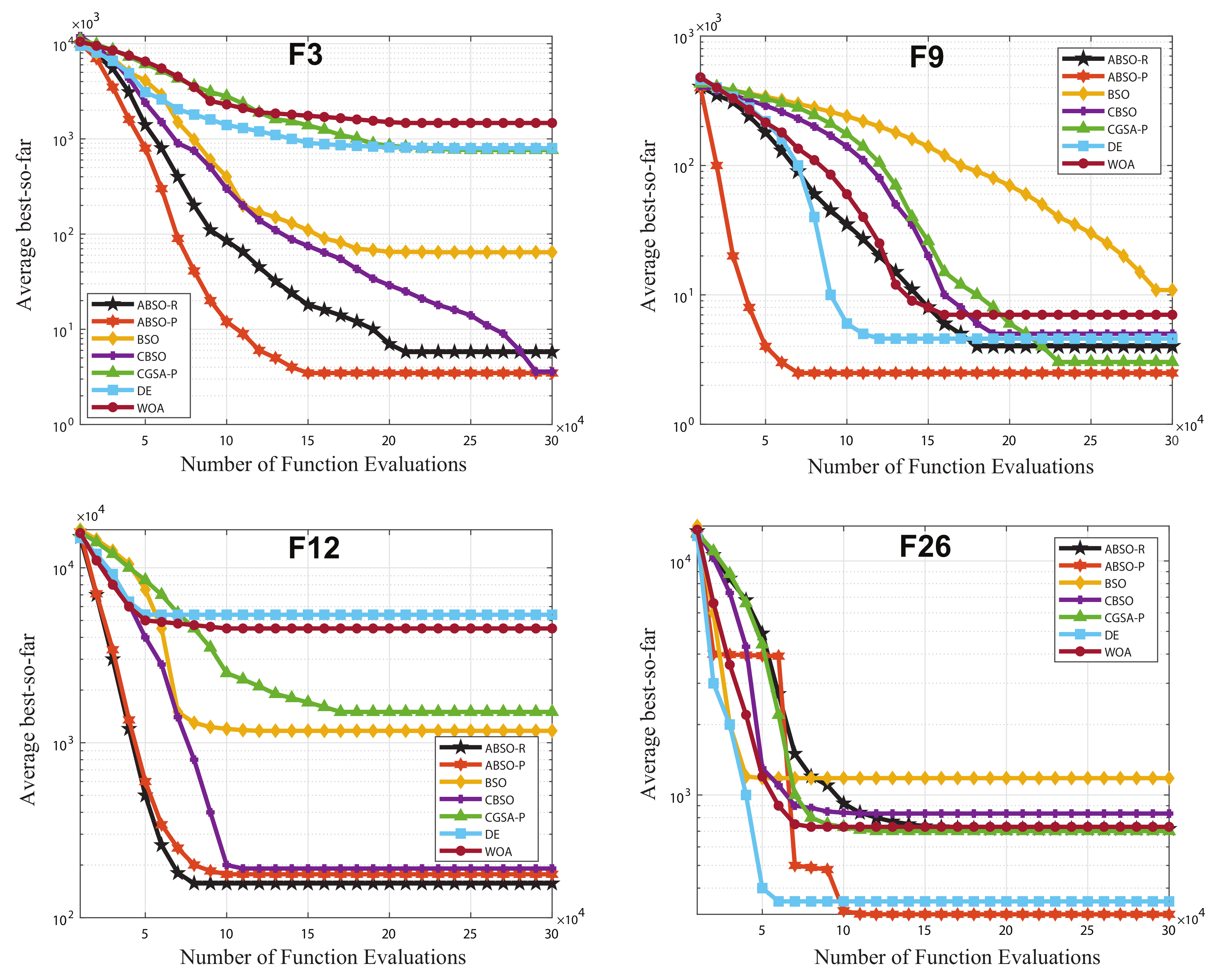
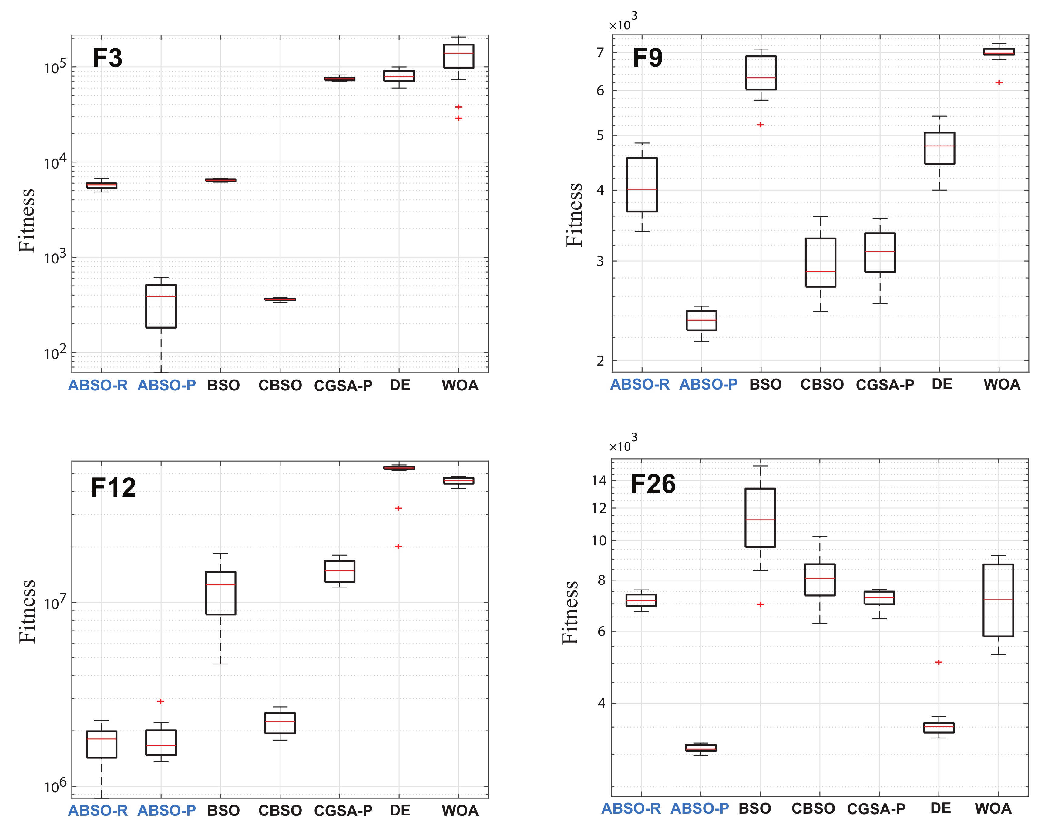
To more intuitively reveal the search performance and stability of the algorithm, we selected 4 representative functions (i.e., F3, F9, F12, and F26) from the 29 functions, and the corresponding convergence graphs and box diagrams are shown in Figure 2 and Figure 3, respectively. The ordinates are logarithmic to show the differences between these algorithms. As shown in Figure 2, when evaluated by the same function, ABSO-P converged rapidly to a good solution. Especially during the first half of iterations in F26, ABSO-P continued to converge downwards based on temporary convergence until the termination of iterations, which indicates that the adaptive self-scaling mechanism in ABSO improved the accuracy of the solution by effectively helping the algorithm jump out of local optima during the search process. Figure 3 shows the box diagrams of each algorithm independently running for 30 times on F3, F9, F12 and F26. ABSO-P showed great stability, while the other algorithms were stable only on certain functions. Based on the above results, the proposed adaptive self-scaling mechanism effectively improves the search ability and efficiency of ABSO, showing strong competitiveness in dealing with various function optimization problems.

6. Computational Complexity

Based on the above experimental and statistical results, ABSO has high-performance global search capabilities. In the previous experimental setup, both BSO and ABSO underwent the same number of function evaluations. However, the computational complexity of BSO and ABSO is worth discussing. If P is the dimension of an algorithm, then the complexity of BSO is defined by initializing the population $O\left(P\right)$ and calculating the fitness of the population $O\left(P\right)$, the complexity of using the $k-means$ algorithm to cluster is $O\left(P^{2}k\right)$, and the complexity of both individual selection and the generation process is $O(P^2$). Thus, the overall complexity of the BSO algorithm is given by

$$O\left(P\right)+O\left(P\right)+O\left(P^{2}k\right)+O\left(P^2\right)+2O\left(P^2\right)+2O\left(P^2\right)=2O\left(P\right)+5O\left(P^2\right)+O\left(P^{2}k\right).$$

(22)

Because ABSO is based on BSO, the complexity of most steps is the same. The difference is that the complexity of generating chaotic variables randomly or in parallel is $O\left(P\right)+O\left(1\right)$. Therefore, the algorithm complexity of ABSO is

$$O\left(P\right)+O\left(1\right)+O\left(P\right)+O\left(P^{2}k\right)+O\left(P^2\right)+2O\left(P^2\right)+2O\left(P^2\right)=2O\left(P\right)+5O\left(P^2\right)+O\left(P^{2}k\right)+O\left(1\right).$$

(23)

According to the above computational complexity, the complexity of both BSO and ABSO is $O\left(P^{2}k\right)$, meaning that ABSO can perform better than BSO without a higher computational cost.

7. Conclusions

Due to the problems of BSO such as premature convergence and an imbalance between global mining and local development in the search process, we proposed the BSO algorithm with an improved adaptive search range, i.e., ABSO-R and ABSO-P, based on the adaptive self-scaling chaotic search strategy. From the experimental results for 29 test functions, ABSO showed a strong competitiveness and great stability compared with existing algorithms (e.g., BSO, CBSO, CGSA-P, DE, and WOA). In particular, by effectively adjusting the balance between the global and local searches, ABSO showed a superior performance in complex optimization. In future work, we will explore the adaptation of parameters in the CLS mechanism to enhance the robustness of the adaptive CLS in solving multimodal functions and engineering problems and therefore apply this approach to more practical optimization problems.

References

- Yin, P.Y.; Chuang, Y.L. Adaptive memory artificial bee colony algorithm for green vehicle routing with cross-docking. Appl. Math. Model. 2016, 40, 9302–9315. [Google Scholar] [CrossRef]
- Ziarati, K.; Akbari, R.; Zeighami, V. On the performance of bee algorithms for resource-constrained project scheduling problem. Appl. Soft Comput. 2011, 11, 3720–3733. [Google Scholar] [CrossRef]
- Chen, J.; Cheng, S.; Chen, Y.; Xie, Y.; Shi, Y. Enhanced brain storm optimization algorithm for wireless sensor networks deployment. In International Conference in Swarm Intelligence; Springer: Cham, Switzerland, 2015; pp. 373–381. [Google Scholar]
- Li, L.; Tang, K. History-based topological speciation for multimodal optimization. IEEE Trans. Evol. Comput. 2014, 19, 136–150. [Google Scholar] [CrossRef]
- Yang, G.; Wu, S.; Jin, Q.; Xu, J. A hybrid approach based on stochastic competitive Hopfield neural network and efficient genetic algorithm for frequency assignment problem. Appl. Soft Comput. 2016, 39, 104–116. [Google Scholar] [CrossRef]
- Bianchi, L.; Dorigo, M.; Gambardella, L.M.; Gutjahr, W.J. A survey on metaheuristics for stochastic combinatorial optimization. Nat. Comput. 2009, 8, 239–287. [Google Scholar] [CrossRef] [Green Version]
- Qin, A.K.; Huang, V.L.; Suganthan, P.N. Differential evolution algorithm with strategy adaptation for global numerical optimization. IEEE Trans. Evol. Comput. 2008, 13, 398–417. [Google Scholar] [CrossRef]
- Price, K.V. Differential evolution. In Handbook of Optimization; Springer: Berlin/Heidelberg, Germany, 2013; pp. 187–214. [Google Scholar]
- Das, S.; Suganthan, P.N. Differential evolution: A survey of the state-of-the-art. IEEE Trans. Evol. Comput. 2010, 15, 4–31. [Google Scholar] [CrossRef]
- Poli, R.; Kennedy, J.; Blackwell, T. Particle swarm optimization. Swarm Intell. 2007, 1, 33–57. [Google Scholar] [CrossRef]
- Kennedy, J.; Eberhart, R. Particle swarm optimization. In Proceedings of the ICNN’95-International Conference on Neural Networks, Perth, WA, Australia, 27 November–1 December 1995; Volume 4, pp. 1942–1948. [Google Scholar]
- Shi, Y. Particle swarm optimization: Developments, applications and resources. In Proceedings of the 2001 Congress on Evolutionary Computation, Seoul, Korea, 27–30 May 2001; Volume 1, pp. 81–86. [Google Scholar]
- Wang, Y.; Gao, S.; Yu, Y.; Cai, Z.; Wang, Z. A gravitational search algorithm with hierarchy and distributed framework. Knowl. Based Syst. 2021, 218, 106877. [Google Scholar] [CrossRef]
- Ji, J.; Gao, S.; Wang, S.; Tang, Y.; Yu, H.; Todo, Y. Self-adaptive gravitational search algorithm with a modified chaotic local search. IEEE Access 2017, 5, 17881–17895. [Google Scholar] [CrossRef]
- Wang, Y.; Yu, Y.; Gao, S.; Pan, H.; Yang, G. A hierarchical gravitational search algorithm with an effective gravitational constant. Swarm Evol. Comput. 2019, 46, 118–139. [Google Scholar] [CrossRef]
- Mirjalili, S.; Lewis, A. The whale optimization algorithm. Adv. Eng. Softw. 2016, 95, 51–67. [Google Scholar] [CrossRef]
- Mafarja, M.M.; Mirjalili, S. Hybrid whale optimization algorithm with simulated annealing for feature selection. Neurocomputing 2017, 260, 302–312. [Google Scholar] [CrossRef]
- Aljarah, I.; Faris, H.; Mirjalili, S. Optimizing connection weights in neural networks using the whale optimization algorithm. Soft Comput. 2018, 22, 1–15. [Google Scholar] [CrossRef]
- Cheng, C.Y.; Pourhejazy, P.; Ying, K.C.; Lin, C.F. Unsupervised Learning-based Artificial Bee Colony for minimizing non-value-adding operations. Appl. Soft Comput. 2021, 105, 107280. [Google Scholar] [CrossRef]
- Ji, J.; Song, S.; Tang, C.; Gao, S.; Tang, Z.; Todo, Y. An artificial bee colony algorithm search guided by scale-free networks. Inf. Sci. 2019, 473, 142–165. [Google Scholar] [CrossRef]
- Yao, X. A review of evolutionary artificial neural networks. Int. J. Intell. Syst. 1993, 8, 539–567. [Google Scholar] [CrossRef]
- Tang, C.; Ji, J.; Tang, Y.; Gao, S.; Tang, Z.; Todo, Y. A novel machine learning technique for computer-aided diagnosis. Eng. Appl. Artif. Intell. 2020, 92, 103627. [Google Scholar] [CrossRef]
- Ji, J.; Gao, S.; Cheng, J.; Tang, Z.; Todo, Y. An approximate logic neuron model with a dendritic structure. Neurocomputing 2016, 173, 1775–1783. [Google Scholar] [CrossRef]
- Ji, J.; Song, Z.; Tang, Y.; Jiang, T.; Gao, S. Training a dendritic neural model with genetic algorithm for classification problems. In Proceedings of the 2016 International Conference on Progress in Informatics and Computing (PIC), Shanghai, China, 23–25 December 2016; pp. 47–50. [Google Scholar]
- Song, S.; Gao, S.; Chen, X.; Jia, D.; Qian, X.; Todo, Y. AIMOES: Archive information assisted multi-objective evolutionary strategy for ab initio protein structure prediction. Knowl. Based Syst. 2018, 146, 58–72. [Google Scholar] [CrossRef]
- Song, Z.; Tang, Y.; Chen, X.; Song, S.; Song, S.; Gao, S. A preference-based multi-objective evolutionary strategy for ab initio prediction of proteins. In Proceedings of the 2017 International Conference on Progress in Informatics and Computing (PIC), Nanjing, China, 15–17 December 2017; pp. 7–12. [Google Scholar]
- Song, S.; Ji, J.; Chen, X.; Gao, S.; Tang, Z.; Todo, Y. Adoption of an improved PSO to explore a compound multi-objective energy function in protein structure prediction. Appl. Soft Comput. 2018, 72, 539–551. [Google Scholar] [CrossRef]
- Song, Z.; Tang, Y.; Ji, J.; Todo, Y. Evaluating a dendritic neuron model for wind speed forecasting. Knowl. Based Syst. 2020, 201, 106052. [Google Scholar] [CrossRef]
- Song, Z.; Tang, C.; Ji, J.; Todo, Y.; Tang, Z. A Simple Dendritic Neural Network Model-Based Approach for Daily PM2.5 Concentration Prediction. Electronics 2021, 10, 373. [Google Scholar] [CrossRef]
- Song, Z.; Zhou, T.; Yan, X.; Tang, C.; Ji, J. Wind Speed Time Series Prediction Using a Single Dendritic Neuron Model. In Proceedings of the 2020 2nd International Conference on Machine Learning, Big Data and Business Intelligence (MLBDBI), Taiyuan, China, 23–25 October 2020; pp. 140–144. [Google Scholar]
- Ji, J.; Song, S.; Tang, Y.; Gao, S.; Tang, Z.; Todo, Y. Approximate logic neuron model trained by states of matter search algorithm. Knowl. Based Syst. 2019, 163, 120–130. [Google Scholar] [CrossRef]
- Todo, Y.; Tang, Z.; Todo, H.; Ji, J.; Yamashita, K. Neurons with multiplicative interactions of nonlinear synapses. Int. J. Neural Syst. 2019, 29, 1950012. [Google Scholar] [CrossRef]
- Shi, Y. Brain storm optimization algorithm. In International Conference in Swarm Intelligence; Springer: Berlin/Heidelberg, Germany, 2011; pp. 303–309. [Google Scholar]
- Sun, C.; Duan, H.; Shi, Y. Optimal satellite formation reconfiguration based on closed-loop brain storm optimization. IEEE Comput. Intell. Mag. 2013, 8, 39–51. [Google Scholar] [CrossRef]
- Duan, H.; Li, C. Quantum-behaved brain storm optimization approach to solving Loney’s solenoid problem. IEEE Trans. Magn. 2014, 51, 1–7. [Google Scholar] [CrossRef]
- Qiu, H.; Duan, H. Receding horizon control for multiple UAV formation flight based on modified brain storm optimization. Nonlinear Dyn. 2014, 78, 1973–1988. [Google Scholar] [CrossRef]
- Guo, X.; Wu, Y.; Xie, L.; Cheng, S.; Xin, J. An adaptive brain storm optimization algorithm for multiobjective optimization problems. In International Conference in Swarm Intelligence; Springer: Cham, Switzerland, 2015; pp. 365–372. [Google Scholar]
- Guo, X.; Wu, Y.; Xie, L. Modified brain storm optimization algorithm for multimodal optimization. In International Conference in Swarm Intelligence; Springer: Cham, Switzerland, 2014; pp. 340–351. [Google Scholar]
- Sun, Y. A hybrid approach by integrating brain storm optimization algorithm with grey neural network for stock index forecasting. Abstr. Appl. Anal. 2014, 2014, 759862. [Google Scholar] [CrossRef]
- Yu, Y.; Gao, S.; Cheng, S.; Wang, Y.; Song, S.; Yuan, F. CBSO: A memetic brain storm optimization with chaotic local search. Memetic Comput. 2018, 10, 353–367. [Google Scholar] [CrossRef]
- Li, C.; Duan, H. Information granulation-based fuzzy RBFNN for image fusion based on chaotic brain storm optimization. Optik 2015, 126, 1400–1406. [Google Scholar] [CrossRef]
- Song, Z.; Gao, S.; Yu, Y.; Sun, J.; Todo, Y. Multiple chaos embedded gravitational search algorithm. IEICE Trans. Inf. Syst. 2017, 100, 888–900. [Google Scholar] [CrossRef] [Green Version]
- GGarcía, S.; Fernández, A.; Luengo, J.; Herrera, F. Advanced nonparametric tests for multiple comparisons in the design of experiments in computational intelligence and data mining: Experimental analysis of power. Inf. Sci. 2010, 180, 2044–2064. [Google Scholar] [CrossRef]
- Alcalá-Fdez, J.; Sanchez, L.; Garcia, S.; del Jesus, M.J.; Ventura, S.; Garrell, J.M.; Herrera, F. KEEL: A software tool to assess evolutionary algorithms for data mining problems. Soft Comput. 2009, 13, 307–318. [Google Scholar] [CrossRef]
- Wolf, A.; Swift, J.B.; Swinney, H.L.; Vastano, J.A. Determining Lyapunov exponents from a time series. Phys. D Nonlinear Phenom. 1985, 16, 285–317. [Google Scholar] [CrossRef] [Green Version]
Figure 1.
Twelve common chaotic maps.
Figure 2.
Convergence of the optimal solution of the proposed algorithm on test functions F3, F9, F12, and F26.
Figure 3.
Box diagrams of each algorithm independently run 30 times on test functions F3, F9, F12, and F26.