
Adaptive Supply Chain: Demand–Supply Synchronization Using Deep Reinforcement Learning


1
Faculty of Engineering and Information Technology, Kazakh-German University, Pushkin 111, Almaty 050010, Kazakhstan
2
Center for Transportation & Logistics, Massachusetts Institute of Technology, 1 Amherst Street, Cambridge, MA 02142, USA
3
Faculty of Engineering, Transport and Telecommunication Institute, Lomonosova 1, LV-1019 Riga, Latvia
*
Author to whom correspondence should be addressed.
†
These authors contributed equally to this work.
Algorithms 2021, 14(8), 240; https://0-doi-org.brum.beds.ac.uk/10.3390/a14080240
Submission received: 21 July 2021
/
Revised: 11 August 2021
/
Accepted: 12 August 2021
/
Published: 15 August 2021
(This article belongs to the Section Algorithms for Multidisciplinary Applications)
Abstract
:Adaptive and highly synchronized supply chains can avoid a cascading rise-and-fall inventory dynamic and mitigate ripple effects caused by operational failures. This paper aims to demonstrate how a deep reinforcement learning agent based on the proximal policy optimization algorithm can synchronize inbound and outbound flows and support business continuity operating in the stochastic and nonstationary environment if end-to-end visibility is provided. The deep reinforcement learning agent is built upon the Proximal Policy Optimization algorithm, which does not require hardcoded action space and exhaustive hyperparameter tuning. These features, complimented with a straightforward supply chain environment, give rise to a general and task unspecific approach to adaptive control in multi-echelon supply chains. The proposed approach is compared with the base-stock policy, a well-known method in classic operations research and inventory control theory. The base-stock policy is prevalent in continuous-review inventory systems. The paper concludes with the statement that the proposed solution can perform adaptive control in complex supply chains. The paper also postulates fully fledged supply chain digital twins as a necessary infrastructural condition for scalable real-world applications.
1. Introduction
The 21st century has begun under the aegis of growing stored data quantities and processing power. This trend eventually resulted in the advent of a machine learning approach capable of leveraging the increased computational resource well-known as deep learning [1]. Despite the temporal crisis in the semiconductor industry, this trend is expected to continue. Currently, a multitude of nontrivial and vitally crucial tasks for logistics on operational and managerial levels have been mastered by deep learning models within the supervised learning paradigm. Under the supervised learning paradigm, deep learning models map data points to the associated labels. However, the potential of deep learning extends far beyond classical supervised learning. Deep reinforcement learning (DRL) takes advantage of the deep artificial neural network architectures to explore possible sequences of actions and associate them with long-term rewards. This appears to be a powerful computational framework for experience-driven autonomous learning [2]. As a result, an adaptive controller based on this principle, also known as an RL agent, can learn how to operate in dynamic and frequently stochastic environments.
DRL has already demonstrated remarkable performance in the fields of autonomous aerial vehicles [3], road traffic navigation [4], autonomous vehicles [5], and robotics [6]. However, what served as the inspiration for this work is the ability of systems based on DRL to master computer games at a level significantly superior to that of a professional human player. Many skeptics can undervalue the astonishing success of AlphaZero in mastering such classic board games as chess, shogi, and go through self-play [7] by pointing out the relative simplicity of rules and determinism of games. However, it appears that DRL is capable of mastering video games that partially capture and reflect the complexity of the real world. Notable examples include Dota 2 [8], StarCraft 2 [9], and Minecraft [10]. On the one hand, computer games are rich and challenging domains for testing DRL techniques. On the other hand, the complexity of the mentioned games can be characterized by long-term planning horizons, partial observability, imperfect information, and high dimensionality of state and action spaces. The mentioned traits often characterize complex supply chains and distribution systems. Given these facts, a central research question arises: “Can the fundamental principles behind DRL be applied to control problems in supply chain management?”
Modern supply chains are highly complex systems that continually make business-critical decisions to stay competitive and adaptive in dynamic environments. Adaptive control in such systems is applied to ensure delivery to end customers with minimal delays and interruptions and avoid unnecessary costs. This objective cannot be achieved without supply chain synchronization, which is defined as real-time coordination of production scheduling, inventory control, and delivery plans among a multitude of individual supply chain participants that frequently spread across the globe. Since inventory on hand is the difference between inbound and outbound commodity flows, proper inventory control is a pivotal element of supply chain synchronization. For example, higher inventory levels allow one to maintain higher customer service levels, but they are associated with extra costs that propagate across the supply chain to the end consumers in the form of the higher price [11]. Therefore, the full potential of the supply chain is unlocked if and only if it becomes synchronized, namely, all the critical stakeholders obtain accurate real-time data, identify weaknesses, streamline processes, and mitigate risk. In this regard, a synchronized supply chain is akin to the gear and cog that operate in harmony. Even if one gear suddenly stops turning, it can critically undermine the synchronization of the entire system, and eventually, the other gears will become ineffective.
Synchronized supply chains can avoid a cascading rise-and-fall inventory dynamic widely known as the “bullwhip effect” [12] and mitigate ripple effects caused by operational failures [13]. Indeed, a DRL agent can only perform adaptive coordination along the whole supply chain if end-to-end visibility is ensured. Shocks and disruptions amid the COVID-19 pandemic, along with post-pandemic recoveries, can become a catalyst for necessary changes in information transparency and global coordination [14]. This paper aims to demonstrate how DRL can synchronize inbound and outbound flows and support business continuity operating in a stochastic environment if end-to-end visibility is provided.
2. Related Work and Novelty
Among the related works, it is worth highlighting [15] one that demonstrated the efficiency of Q-learning for dynamic inventory control in a four-echelon supply chain model that included a retailer, distributor, and manufacturer. The supply chain simulation was distinguished by nonstationary demand under a Poisson distribution. Barat et al. presented an RL agent based on the A2C algorithm for closed-loop replenishment control in supply chains [16]. Zhao et al. adapted the Soar RL algorithm to reduce the operational risk in resilient and agile logistics enterprises. The problem was modeled as an asymmetrical wargame environment [17]. Wang et al. applied a DRL agent to the supply chain synchronization problem under demand uncertainty [18]. In the recent paper, Perez et al. compared several techniques, including RL on a single product, a multi-period centralized system under stochastic stationary consumer demand [11].
An RL agent capable of playing the beer distribution game was proposed in a recent paper [19]. The beer distribution game is widely used in supply chain management education to demonstrate the importance of supply chain coordination. The RL agent is built upon deep Q-learning and is not provided any preliminary information on costs or other settings of the simulated environments. Therefore, it is imperative to highlight the OR-Gym [20], an open-source library that contains common operation research problems in the form of RL environments, including one used in this study.
In numerical experiments presented further in this paper, the DRL agent is built upon the proximal policy optimization (PPO) algorithm, which does not require exhaustive hyperparameter tuning. Besides, the implementation of PPO used in this paper does not require hardcode action space. These features, complimented with a simple and straightforward supply chain model used as an RL environment, result in a general and task unspecific approach to adaptive control in multi-echelon supply chains. It is essential to highlight that numerical experiments are conducted using a simplified supply chain model, which is sufficient at the proof-of-concept stage. However, the simplified assumptions cannot fully capture all the complexity of many real-world supply chains.
3. Methodology
This section introduces the fundamentals behind RL and the Markov decision process (MDP). After that, the supply chain environment (SCE) is described. Lastly, the section sheds light on the PPO algorithm.
3.1. Supply Chain Environment
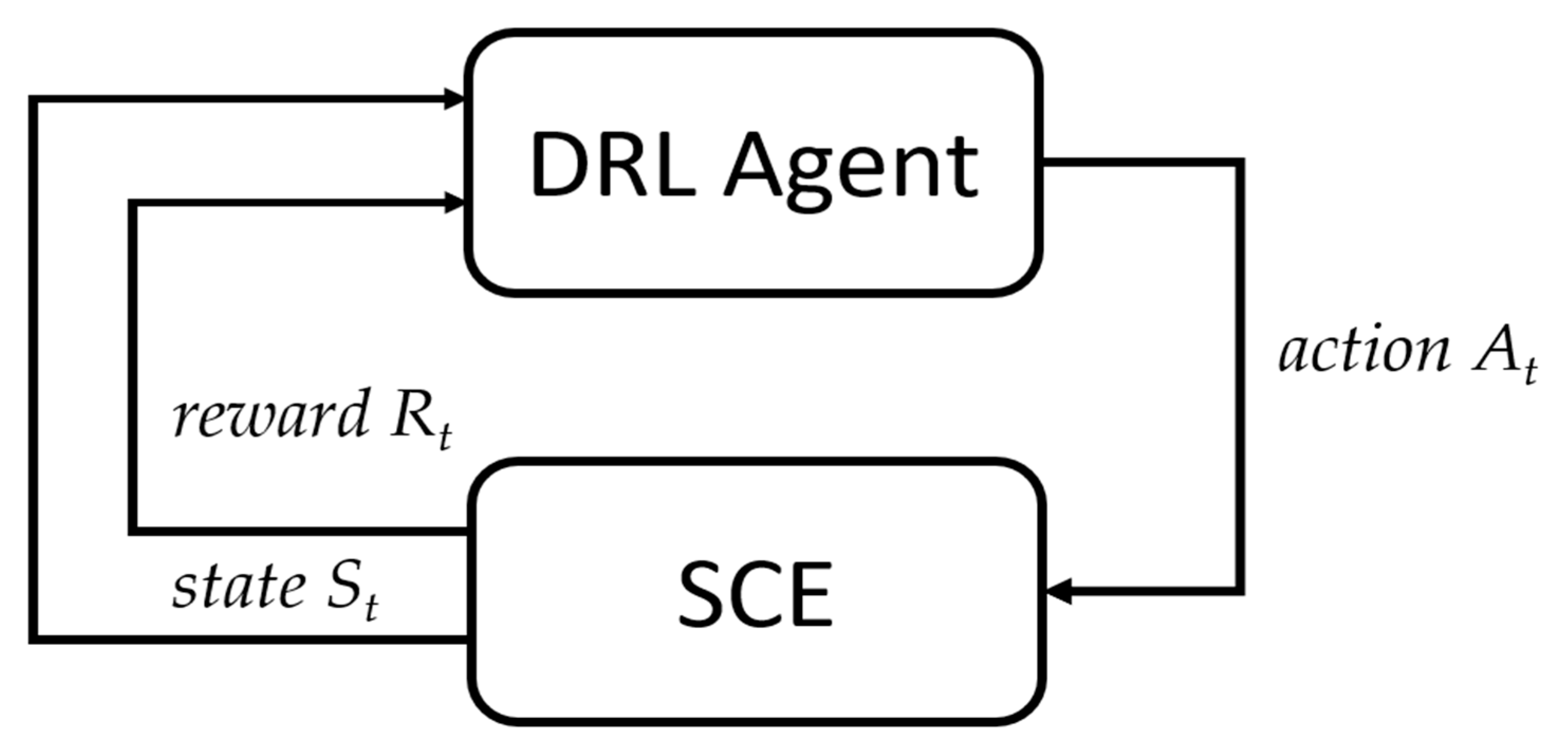
SCE can be naturally formulated as MDP. MDP serves as the mathematical foundation and straightforward framework for goal-directed learning from interaction with a virtual environment. An RL agent interacts with an environment over multiple time steps (Figure 1).
The RL agent and environment interact at each instance of a sequence of discrete time steps t ∈ T. At each time step t, the agent receives a representation of the environmental state St ∈ S and numerical reward Rt ∈ R in response to a performed action At ∈ A. After that, the agent finds itself in a new state St+1. The sequence of states, actions, and rewards gives rise to a trajectory of the following form S0, A0, R1, S1, A1, R2, S2, A2, R3, …, Sn, where Sn stands for the terminal state [21]. At each time step, the agent conducts multiple trials with the stochastic environment (episodes). The agent observes St and Rt performing actions under a policy π that maps states to actions. In such settings, the agent’s goal is to learn a policy that leads to the highest cumulative reward. In this regard, RL can be considered a stochastic optimization process [22].
The function p(.) describes the probability of an RL agent finding itself in a particular state S* and obtaining the particular reward R*, when taking action A* in state St. This dynamics within the MDP framework can be described by the following equation:
In SCE, the agent must decide how many goods to order for each stage m at each time step t. The action At is an integer value corresponding to each reorder quantity at each stage along the supply chain. The state St constitutes a vector that includes the inventory level for each stage and the previously taken actions. Thus, the RL agent attempts to synchronize the supply chain so that the total revenue over the time horizon is maximized (see Equation (7)).
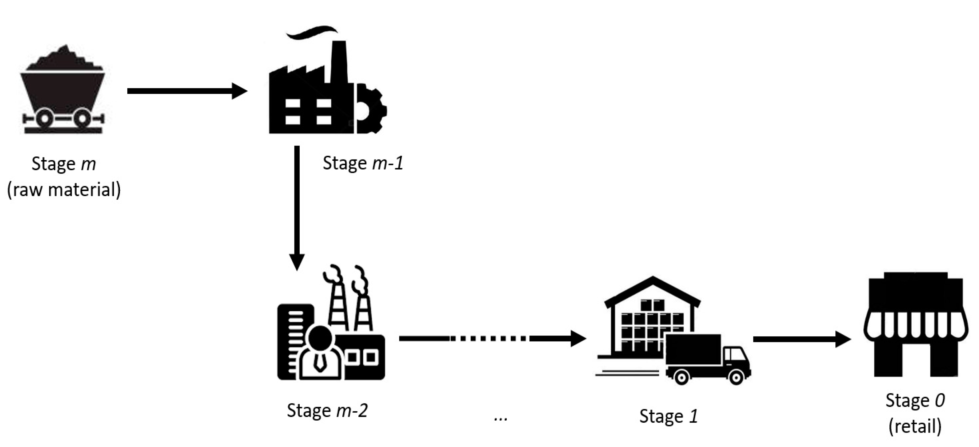
SCE is based on the seminal work [23] and implemented within the OR-gym, an open-source collection of RL environments related to logistics and operations research [20]. SCE represents a single-product multi-echelon supply chain model. The model makes several assumptions. The tradable goods do not perish over time, and replenishment sizes are integers. Economic agents involved in the supply chains can be represented as stages M = {0, 1, …, mend}. Stage 0 stands for a retailer that fulfills a customer’s demand. Stage mend stands for a raw material supplier. Stages from 1 to mend−1 represent intermediaries involved in the product lifecycle, for example, wholesalers and manufacturers (Figure 2). One unit from the previous stage is transformed into one unit in the following stage until the final product is obtained. Replenishment lead times between stages are constant, measured in days, and include production and transportation times. Both production and inventory capacities are limited for all stages except the last one (raw material supply is assumed to be infinite). During the simulation at each time step t ∈ T, the following sequence of events take place:
- All the stages except the raw material pool place replenishment orders.
- Replenishment orders are satisfied according to available production and inventory capacity.
- Demand arises and is satisfied according to the inventory on hand at stage 0 (retailer).
- Unsatisfied demand and replenishment orders are lost (backlogging is not allowed).
- Holding costs are charged for each unit of excess inventory.
∀ m ∈ M and ∀ t ∈ T, the SCE dynamics is governed by the following set of equations:
where at the beginning of each period t ∈ T at each stage m ∈ M, I denotes inventory on hand. V stands for the commodities that are ordered and on the way (pipeline inventory). corresponds to the accepted reorder quantity, and is the requested reorder quantity. L stands for replenishment lead time between stages. Demand D is a discrete random variable under Poisson distribution. The sales ζ at each period equal to the customer demand satisfied by the retailer at stage 0 and the accepted reorder quantities from the succeeding stages from 1 to mend. U denotes unfulfilled demand and unfulfilled reorder requests. The net profit NP equals sales revenue minus procurement costs, the penalty for unfulfilled demand, and inventory holding costs. , r, k, and h stand for the unit sales price, unit procurement cost, unit penalty for unfulfilled demand, and unit inventory holding costs. If production capacity and inventory level are sufficient (do not exceed capacity constraints c), would be equal to . However, if capacities are insufficient, it imposes an upper bound on the reorder quantity that can be accepted. It is assumed that the inventory of raw materials at stage mend is infinite.
It is important to emphasize that besides the non-perishability of goods and integer replenishment sizes, SCE makes a strong assumption regarding end-to-end visibility. Namely, information is assumed to be complete, accurate, and available along the supply chain. This assumption appears to be unrealistic in many real-world applications, given the current digitalization level. This assumption can hold if a single company controls the vast majority of a supply chain, let us say, from farm to fork or from quartz sand to microchip. However, the assumption is false for a larger swath of supply chains. We primarily see an outsourcing trend, according to which companies mainly focus on those activities in the supply chain where they have a distinct advantage and outsource everything else. Therefore, the pervasive adoption of the fully fledged supply chain digital twins or other technologies capable of providing information transparency and end-to-end visibility is a necessary infrastructural condition for real-world implementation. Furthermore, assuming that information transparency is partially provided, such SCE can serve as a proxy for real-world applications in supply chain management to gauge generalized algorithm performance.
3.2. Proximal Policy Optimization Algorithm
PPO is applied to train the RL agent. PPO is developed by the OpenAI team and distinguished by simple implementation, generality, and low sample complexity (the number of training samples that the RL agent needs to learn a target function with a sufficient degree of accuracy). On the other hand, the vast majority of machine learning algorithms require hyperparameters that must be finetuned external to the learning algorithm itself. In this regard, an extra advantage of PPO is that it can provide solid results with either default parameters or relatively little hyperparameter tuning [24].
PPO is an actor-critic approach to DRL. It uses two deep artificial neural networks, one to generate actions at each time step (actor) and one to predict the corresponding rewards (critic). The actor learns a policy that produces a probability distribution of feasible actions. On the other hand, the critic learns to estimate the reward function for given states and actions. The difference between the reward predicted by the critic with parameters θ and the actual reward received from the environment is reflected in the loss function Loss(θ). PPO limits the update of the parameters by clipping the loss function Equation (8). This loss function constitutes the distinguishing feature of PPO and demonstrates more stable learning compared to other state-of-the-art policy gradient methods across various benchmarks.
where πk−1 and πk denote the previous policy and the new policy. k stands for the number of updates to the policy since initialization. The function cl(.) imposes the constraint of form 1 − ε ≤ πk−1/πk ≤ 1 + ε. ε is a tunable hyperparameter that prevents policy updates that are too radical. The advantage estimation of the state is the sum of the discounted prediction errors over T time steps , where is the difference between the actual and the estimated rewards provided by the critic artificial neural network, also known as the temporal difference error. stands for the discount rate. Algorithm 1 demonstrates the implementation of PPO in Actor-Critic style.
| Algorithm 1 Actor–Critic Style within PPO |
| for iteration = 1, 2, ... do for actor = 1, 2, ..., N do Run policy πθold in environment for T timesteps Compute advantage estimates , ..., end for Optimize surrogate Loss with regard to θ θold ← θ end for |
The implemented PPO uses fixed-length trajectory segments. In each iteration, each of N actors collects T timesteps of data in parallel. Then, the surrogate loss function is obtained and can be further optimized with mini-batch stochastic gradient descent. Therefore, the algorithm aims to compute an update at each iteration that minimizes the loss function while ensuring the relatively small deviation from the previous policy. As a result, the algorithm reaches a balance between ease of implementation and tuning and sample complexity.
4. Numerical Experiment
This section describes two numerical experiments with different environment settings. In both experiments, the simulation lasts for 30 periods (modeling days). Furthermore, in both experiments, a DRL agent based on PPO is compared with the base-stock policy, a common approach in classic inventory control theory.
4.1. Implementation and Configurations
The first numeric experiment is conducted with a four-stage supply chain. Table 1 contains the parameters of SCE used in the experiment. The second and the third numeric experiments are conducted with larger four-stage supply chains using longer lead times and generally more challenging environment settings (Table 2 and Table 3). The PPO algorithm is implemented in parallel using the Ray framework. The framework performs actor-based computations orchestrated by a single dynamic execution engine. Besides, Ray is distinguished by a distributed scheduler and fault-tolerant storage framework. The framework demonstrated scaling beyond 1.8 million tasks per second and better performance than alternative solutions for several challenging RL problems [25].
In the numerical experiments, a feed-forward architecture with one hidden layer and 256 neurons is used for actor and critic artificial neural networks. An exponential linear unit is used as an activation function, ε equals 0.3, and the learning rate is set to 10−5.
The PPO algorithm is compared with the base-stock policy, a well-known approach in classic operations research and inventory control theory. The base-stock policy is especially common in continuous-review inventory systems. Even though demand is assumed to be generated by a stationary and independent Poisson process, the base-stock policy can perform well even if this assumption does not hold [26]. The numeric experiment is conducted in a fully reproducible manner using Google Colaboratory, a hosted version of Jupyter Notebooks. Thus, results can be reproduced and verified by anyone [27]. Table 4 provides details on the available computational resources. Teraflops refer to the capability of calculating one trillion floating-point operations per second, a standard GPU performance estimation metric.
4.2. Results
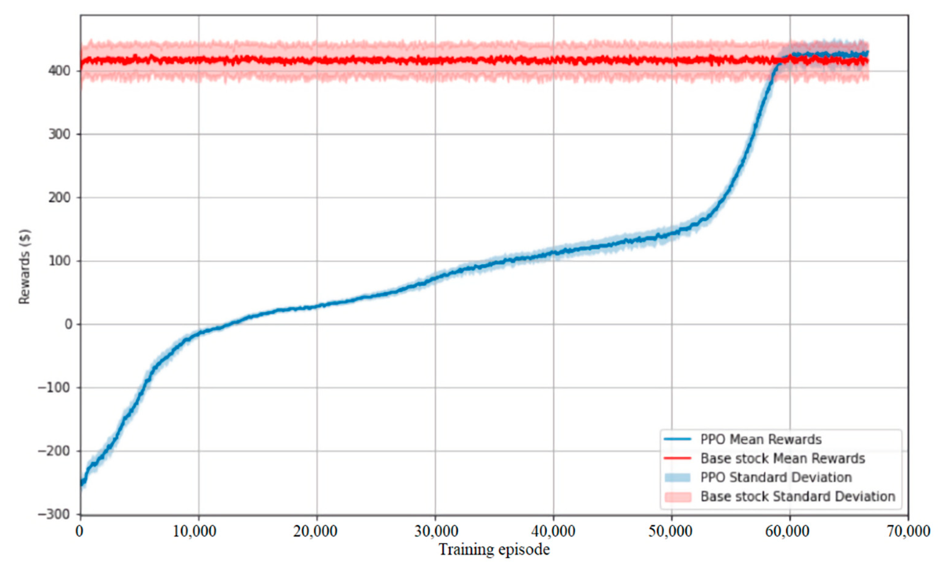
In the first experiment, the base-stock policy used as a benchmark could achieve an average reward of 414.3 abstract monetary units with a standard deviation of 26.5. On the other hand, in 66,000 training episodes, the PPO agent could derive a policy that led to an average reward of 425.6 abstract monetary units, which is 2.7% higher, having a smaller standard deviation of 19.4 at the same time. The training procedure is conducted using GPU and takes 97 min on the hardware mentioned above.
The learning procedure and comparison against the benchmark is demonstrated in Figure 3.
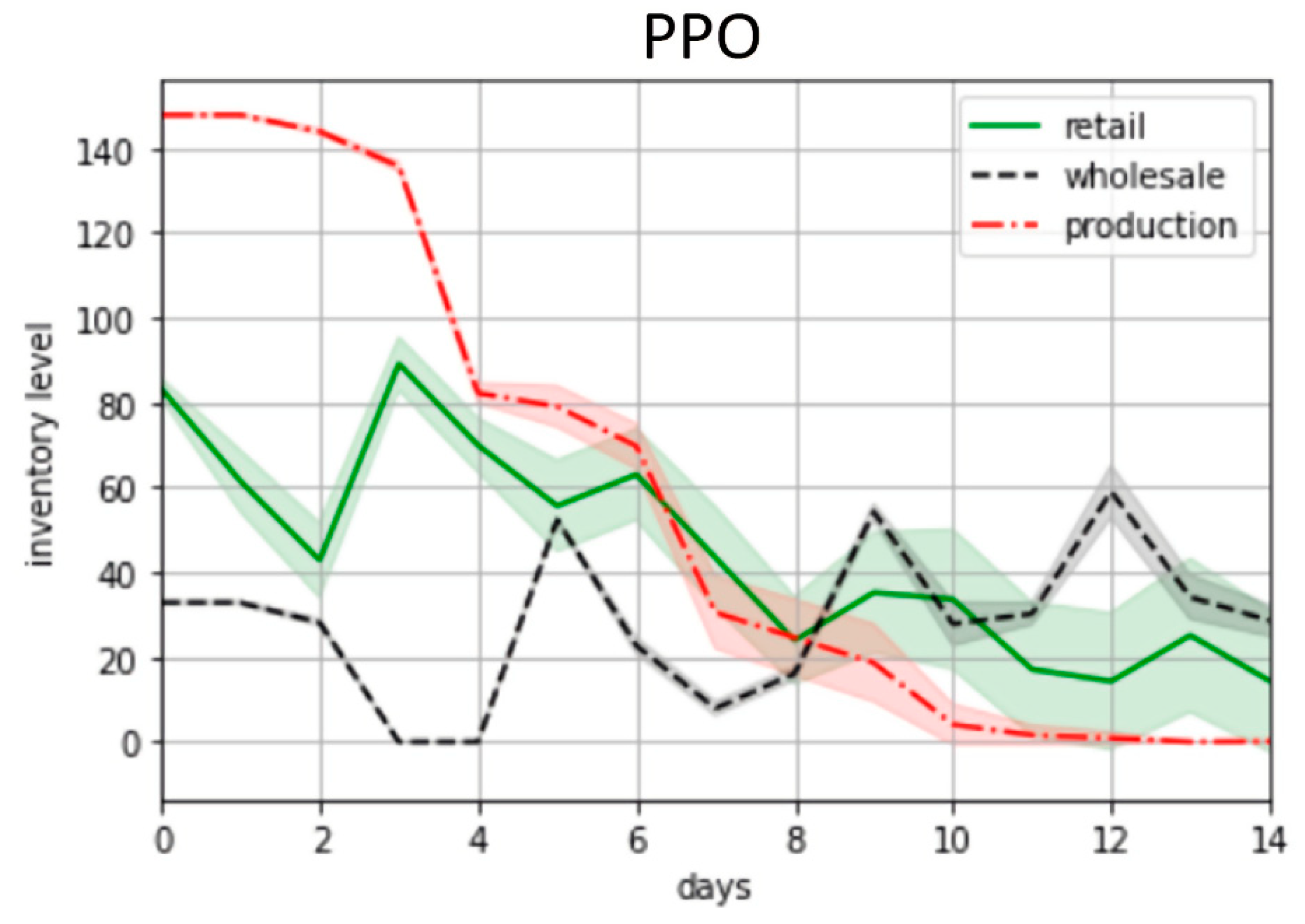
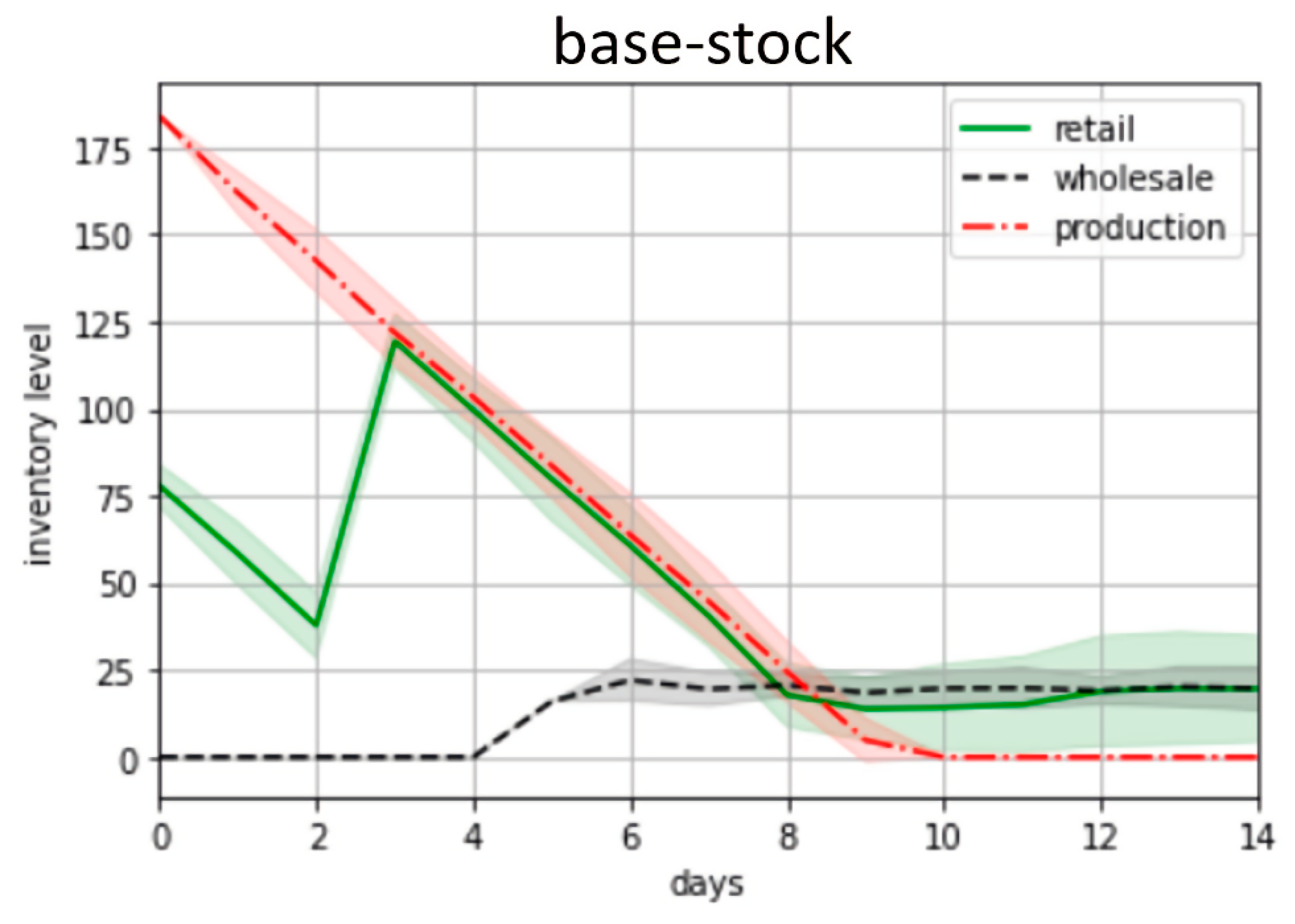
Figure 4 and Figure 5 illustrate the inventory dynamics for two weeks at all the stages under the control of the trained PPO agent and the base-stock policy. It is worth mentioning that the inventory dynamics illustrated in the figures are fundamentally different. Unlike the base-stock policy (Figure 5), the PPO agent derived the control rule that entails notable fluctuations, especially for a retailer and wholesaler (Figure 6). On the one hand, this indicates that the stochastic fluctuations of demand propagate across the supply chain, causing the cycles of overproduction and underproduction. On the other hand, it speaks to the agent’s adaptability and ability to adjust production and distribution.
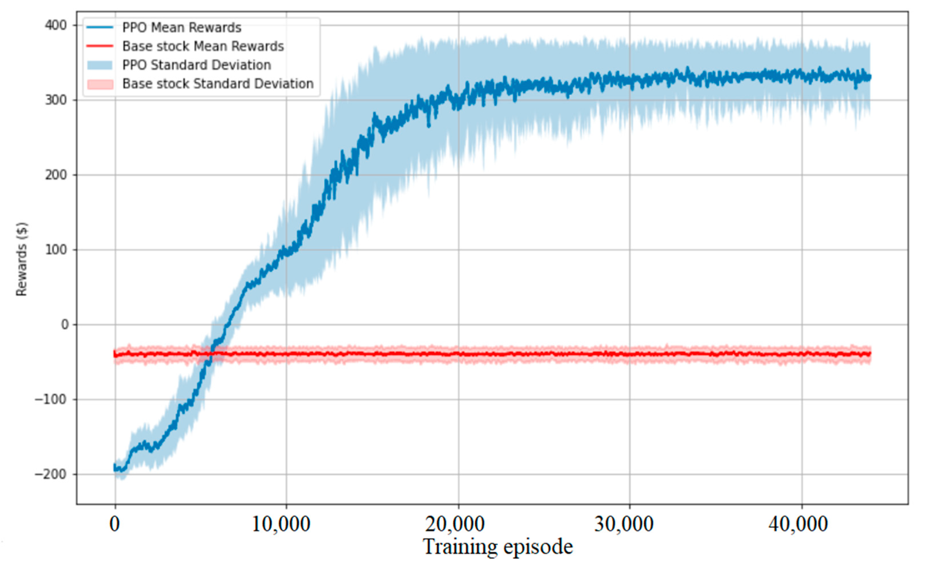
In the second experiment, the PPO agent decisively outcompeted the base-stock policy operation in more challenging environment settings. The training procedure took 79 min (Figure 6).
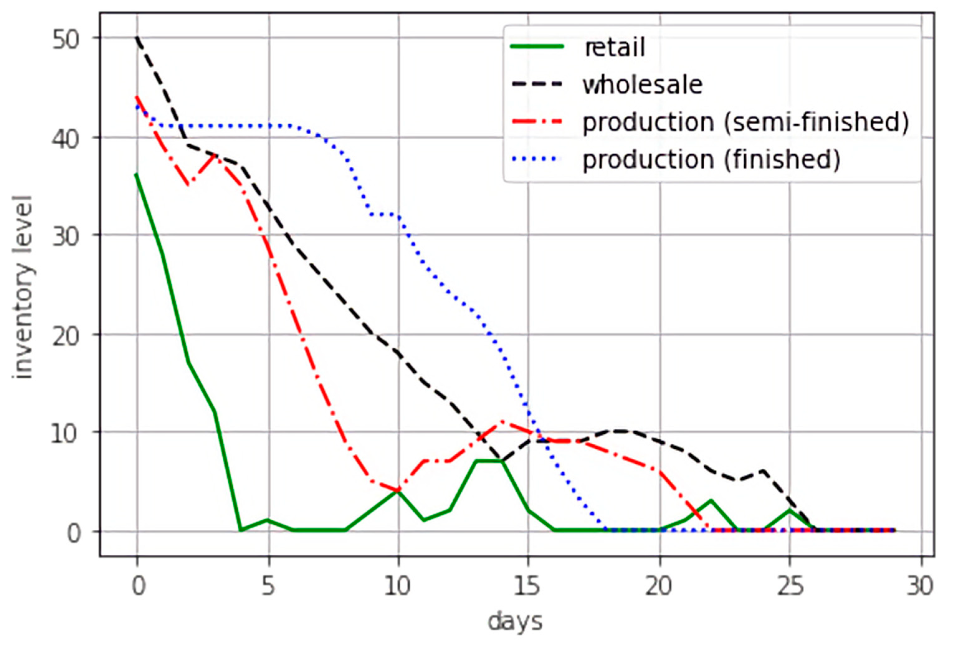
During the third experiment, unusual behavior was observed. The PPO agent took advantage of the policy that terminates ordering additional inventory closer to the end of the simulation run. This strategy can be explained by the fact that the simulation time is limited by 30 days, and the agent, based on its experience, expects that there will not be enough time to sell all the goods, and holding costs associated with excessive inventory will not be paid off. In other words, the policy learned by the agent taking into account the specifics of the SCE. During the training session, the PPO agent was capable of learning the policy, which is a mapping between states and actions that entail maximum expected reward. Figure 7 illustrates this unusual behavior under the control of the trained PPO agent. Indeed, such a problem may be circumvented by modifying the SCE, for example, by adding a “cool down” period equal to the sum of all the lead times to the initial time horizon. The tendency of the RL agent to exploit the mechanics of simulated environments in an unexpected way is quite common and known in the domain of competitive cybersport. Therefore, this phenomenon deserves specific attention during the development of applications for real-world problems.
Nevertheless, even with such an unpredictable solution, the PPO agent managed to adapt and find the policy that entails a positive net profit in the specified environmental setup. The training procedure took 76 min. At the same time, the policy under base-stock did not lead to a profitable outcome (Figure 8). Table 5 summarizes the results of all three numerical experiments. The table contains mean rewards, standard deviations, coefficient of variations, and 95% confidence intervals. The values are reported for the fully trained PPO agent and base-stock policy.
5. Discussion
The PPO algorithm has demonstrated a decisive capability of performing adaptive control in multi-stage supply chains. Among the discovered benefits, it is essential to highlight that the PPO algorithm is general, task unspecific, and does not rely on prior knowledge about the system. Besides, the labor-intense procedure of exhaustive hyperparameter tuning is not required.
Concerning the technical aspects, it is also worth mentioning that PPO implementation and training are straightforward within the contemporary frameworks. However, it is essential to keep in mind that RL agents learn to map from the state of the environment to a choice of action that entails the highest reward. Therefore, their reliance on the simulated environments requires specific attention. In this regard, the simulated environment should not be oversimplified and must capture all the pivotal relations within the elements of a real-world supply chain. The tendency of the learning agent to abuse and exploit simulation mechanics has been discovered in this research and deserves primary consideration in development and deployment. It is also worth emphasizing that a manifold of advanced supply chain models exists in the form of discrete event simulations (DES) [28]. Currently, the vast majority of RL research follows the standard prescribed by the OpenAI Gym framework [29]. In short, an environment has to be a Python class inherited from gym.Env and containing at least such methods as reset and step. The step method takes action as the input and returns a new state and reward value. Thus, it can be considered the fundamental mechanism that advances time. Unlike DES models, the time by default advances with a constant time step. Therefore, in order to produce a standardized RL environment out of DES, the time has to become part of the state, an environment variable observable for an agent. On the other hand, since it is assumed that between consecutive events, no change in the system will take place, the method step has to execute and reschedule the next event in the list. This problem is addressed by Schuderer et al. [30] and, if a standardized and straightforward way of transforming DES models into RL environments is developed, a plethora of the models developed over the past 30 years will become available to RL applications.
Indeed, a DRL agent of that kind can synchronize the supply chain if and only if end-to-end visibility is provided. Besides, planning and real-time control require constant data availability on replenishments, inventory, demand, and capacities [31]. The ultimate fulfillment of these requirements is an advent of a digital replica of a supply chain representing the system state at any given moment in real-time, providing complete end-to-end visibility and the possibility to test contingency plans. This concept is known as a digital supply chain twin [14]. Incorporating RL agents into supply chain digital twins can be considered one of the most promising trajectories for future research.
The capability of a DRL agent to transfer knowledge across multiple environments is considered a critical aspect of intelligent agents and a potential way to artificial general intelligence [32]. The PPO agent demonstrated the ability to learn in different SCEs with the same hyperparameters, which can be considered sufficient at the proof-of-concept stage. This capability can be considered a different generalization type compared to cases in which the trained agent can perform well in unseen environments. However, the agent in the current implementation cannot perform well in the previously unseen configuration of SCE. In this regard, such performance generalization techniques as multi-task learning [33] and policy distillation [34] can be postulated as an additional direction for future research.
Besides, in order to study how the stochasticity in SCE inputs affects the output, in future work, it is essential to conduct a sensitivity analysis of the parameters in the model and the algorithm.
6. Conclusions
The conducted numerical experiments demonstrated the capability to outcompete the base-stock policy. The paper concludes with the statement that the proposed solution can outperform the base-stock policy in adaptive control over stochastic supply chains. In the three-stage supply chain environment, the base-stock policy used as a benchmark could achieve an average reward of 414.3 abstract monetary units with a standard deviation of 26.5. On the other hand, it took the PPO agent 66,000 training episodes to derive a policy that leads to an average reward of 425.6 abstract monetary units, which is 2.7% higher, while also having a smaller standard deviation. In more challenging environments with more extensive supply chains and longer lead times, the PPO agent decisively outperformed the base-stock policy by deriving the policy that entails a positive net profit.
However, the sequence of experiments also revealed the tendency of the learning agent to exploit simulation mechanics. The tendency of the RL agent to exploit the mechanics of simulated environments in an unexpected way is well-known in the domain of competitive cybersport. This phenomenon deserves specific consideration in real-world implementations. The simulated environment should not be oversimplified and must capture all the pivotal relations within the elements of a real-world supply chain or logistic system.
Among the technical advantages, it is essential to highlight that the PPO algorithm is general, task unspecific, does not rely on prior knowledge about the system, and does not require explicitly defined action space or exhaustive hyperparameter tuning. Additionally, its implementation and training are straightforward within the contemporary frameworks. It is worth keeping in mind that RL agents learn to map from the state of the environment to a choice of action that entails the highest reward. Therefore, their reliance on the simulated environments requires specific attention. From the applicability point of view, the assumption of the provided end-to-end visibility may be unrealistic in many real-world applications given the current digitalization level, and the pervasive adoption of the fully fledged supply chain digital twins is a necessary infrastructural condition. Nevertheless, if the information visibility and transparency are achieved, SCE can serve as a proxy for real-world applications in supply chain management to gauge generalized algorithm performance.
Author Contributions
Conceptualization, I.J. and Z.K.; methodology, I.J.; development, I.J.; validation, I.J. and Z.K.; software, I.J.; validation, I.J.; formal analysis, I.J.; project administration, Z.K.; funding acquisition, Z.K. All authors have read and agreed to the published version of the manuscript.
Funding
This research was funded by the Kazakh-German University.
Institutional Review Board Statement
Not applicable.
Informed Consent Statement
Not applicable.
Data Availability Statement
The numeric experiment was conducted in a fully reproducible manner using Google Colaboratory, a hosted version of Jupyter Notebooks. Thus, results can be reproduced and verified by anyone. Executable Colab Notebook: https://colab.research.google.com/drive/1D_E1j10skbohOOA4vbuy9OCw4dqbAW_S?usp=sharing (accessed on 14 August 2021).
Conflicts of Interest
The authors declare no conflict of interest.
References
- Goodfellow, I.; Bengio, Y.; Courville, A.; Bengio, Y. Deep Learning, 2nd ed.; MIT Press: Cambridge, UK, 2016. [Google Scholar]
- Mosavi, A.; Faghan, Y.; Ghamisi, P.; Duan, P.; Ardabili, S.F.; Salwana, E.; Band, S.S. Comprehensive review of deep reinforcement learning methods and applications in economics. Mathematics 2020, 8, 1640. [Google Scholar] [CrossRef]
- Ng, A.; Coates, A.; Diel, M.; Ganapathi, V.; Schulte, J.; Tse, B.; Berger, E.; Liang, E. Autonomous inverted helicopter flight via reinforcement learning. Exp. Robot. 2006, 9, 363–372. [Google Scholar] [CrossRef]
- Fridman, L.; Terwilliger, J.; Jenik, B. Deep traffic: Crowdsourced hyperparameter tuning of deep reinforcement learning systems for multi-agent dense traffic navigation. arXiv 2018, arXiv:1801.02805. [Google Scholar]
- Isele, D.; Rahimi, R.; Cosgun, A.; Subramanian, K.; Fujimura, K. Navigating occluded intersections with autonomous vehicles using deep reinforcement learning. In Proceedings of the 2018 IEEE International Conference on Robotics and Automation (ICRA), Brisbane, Australia, 21–25 May 2018; pp. 2034–2039. [Google Scholar]
- Gu, S.; Holly, E.; Lillicrap, T.; Levine, S. Deep reinforcement learning for robotic manipulation with asynchronous off-policy updates. In Proceedings of the IEEE International Conference on Robotics and Automation (ICRA 2017), Singapore, 29 May–3 June 2017; pp. 3389–3396. [Google Scholar]
- Silver, D.; Hubert, T.; Schrittwieser, J.; Antonoglou, I.; Lai, M.; Guez, A.; Lanctot, M.; Sifre, L.; Kumaran, D.; Graepel, T.; et al. A general reinforcement learning algorithm that masters chess, shogi, and Go through self-play. Science 2018, 362, 1140–1144. [Google Scholar] [CrossRef] [Green Version]
- Berner, C.; Brockman, G.; Chan, B.; Cheung, V.; Debiak, P.; Dennison, C.; Farhi, D.; Fischer, Q.; Hashme, S.; Hesse, C.; et al. Dota 2 with large scale deep reinforcement learning. arXiv 2019, arXiv:1912.06680. [Google Scholar]
- Vinyals, O.; Babuschkin, I.; Czarnecki, W.M.; Mathieu, M.; Dudzik, A.; Chung, J.; Choi, D.H.; Powell, R.; Ewalds, T.; Georgiev, P.; et al. Grandmaster level in StarCraft II using multi-agent reinforcement learning. Nature 2019, 575, 350–354. [Google Scholar] [CrossRef]
- Guss, W.H.; Codel, C.; Hofmann, K.; Houghton, B.; Kuno, N.; Milani, S.; Mohanty, S.P.; Liebana, D.P.; Salakhutdinov, R.; Topin, N.; et al. The MineRL Competition on Sample Efficient Reinforcement Learning using Human Priors. arXiv 2019, arXiv:1904.10079. [Google Scholar]
- Perez, H.D.; Hubbs, C.D.; Li, C.; Grossmann, I.E. Algorithmic Approaches to Inventory Management Optimization. Processes 2021, 9, 102. [Google Scholar] [CrossRef]
- Lee, H.L.; Padmanabhan, V.; Whang, S. Information distortion in a supply chain: The bullwhip effect. Manag. Sci. 1997, 43, 546–558. [Google Scholar] [CrossRef]
- Li, Y.; Chen, K.; Collignon, S.; Ivanov, D. Ripple effect in the supply chain network: Forward and backward disruption propagation, network health and firm vulnerability. Eur. J. Oper. Res. 2021, 291, 1117–1131. [Google Scholar] [CrossRef] [PubMed]
- Ivanov, D.; Dolgui, A. A digital supply chain twin for managing the disruption risks and resilience in the era of Industry 4.0. Prod. Plan. Control 2020, 32, 775–788. [Google Scholar] [CrossRef]
- Mortazavi, A.; Arshadi Khamseh, A.; Azimi, P. Designing of an intelligent self-adaptive model for supply chain ordering management system. Eng. Appl. Artif. Intell. 2015, 37, 207–220. [Google Scholar] [CrossRef]
- Barat, S.; Khadilkar, H.; Meisheri, H.; Kulkarni, V.; Baniwal, V.; Kumar, P.; Gajrani, M. Actor based simulation for closed loop control of supply chain using reinforcement learning. In Proceedings of the 18th International Conference on Autonomous Agents and Multi Agent Systems 2019, Montreal, QC, Canada, 13–17 May 2019; pp. 1802–1804. [Google Scholar]
- Zhao, Y.; Hemberg, E.; Derbinsky, N.; Mata, G.; O’Reilly, U.M. Simulating a Logistics Enterprise Using an Asymmetrical Wargame Simulation with Soar Reinforcement Learning and Coevolutionary Algorithms. In Proceedings of the Genetic and Evolutionary Computation Conference Companion (GECCO’ 21), Lille, France, 10–14 July 2021; pp. 1907–1915. [Google Scholar] [CrossRef]
- Wang, R.; Gan, X.; Li, Q.; Yan, X. Solving a Joint Pricing and Inventory Control Problem for Perishables via Deep Reinforcement Learning. Complexity 2021, 2021, 6643131. [Google Scholar] [CrossRef]
- Oroojlooyjadid, A.; Nazari, M.; Snyder, L.V.; Takac, M. A Deep Q-Network for the Beer Game: Deep Reinforcement Learning for Inventory Optimization. Manuf. Serv. Oper. Manag. 2021, 1–20. [Google Scholar] [CrossRef]
- Hubbs, C.; Perez, H.D.; Sarwar, O.; Sahinidis, N.V.; Grossmann, I.E.; Wassick, J.M. OR-Gym: A Reinforcement Learning Library for Operations Research Problem. arXiv 2020, arXiv:2008.06319. [Google Scholar]
- Sutton, R.S.; Barto, A.G. Reinforcement Learning: An Introduction; MIT Press: Cambridge, MA, USA, 2018. [Google Scholar]
- Bellman, R. A Markovian decision process. J. Math. Mech. 1957, 6, 679–684. [Google Scholar] [CrossRef]
- Glasserman, P.; Tayur, S. Sensitivity analysis for base-stock levels in multiechelon production-inventory systems. Manag. Sci. 1995, 41, 263–281. [Google Scholar] [CrossRef]
- Schulman, J.; Wolski, F.; Dhariwal, P.; Radford, A.; Klimov, O. Proximal policy optimization algorithms. arXiv 2017, arXiv:1707.06347. [Google Scholar]
- Moritz, P.; Nishihara, R.; Wang, S.; Tumanov, A.; Liaw, R.; Liang, E.; Elibol, M.; Yang, Z.; Paul, W.; Jordan, M.I.; et al. Ray: A distributed framework for emerging AI applications. In Proceedings of the 13th Symposium on Operating Systems Design and Implementation (OSDI 18), Carlsbad, CA, USA, 8–10 October 2018; pp. 561–577. [Google Scholar]
- Kapuscinski, R.; Tayur, S. Optimal policies and simulation-based optimization for capacitated production inventory systems. In Quantitative Models for Supply Chain Management; Springer: Berlin/Heidelberg, Germany, 1999; pp. 7–40. [Google Scholar] [CrossRef]
- Executable Colab Notebook: Google Colaboratory. Available online: https://colab.research.google.com/drive/1D_E1j10skbohOOA4vbuy9OCw4dqbAW_S?usp=sharing (accessed on 14 August 2021).
- Jackson, I.; Tolujevs, J.; Kegenbekov, Z. Review of Inventory Control Models: A Classification Based on Methods of Obtaining Optimal Control Parameters. Transp. Telecommun. 2020, 21, 191–202. [Google Scholar] [CrossRef]
- Brockman, G.; Cheung, V.; Pettersson, L.; Schneider, J.; Schulman, J.; Tang, J.; Zaremba, W. Openai gym. arXiv 2016, arXiv:1606.01540. [Google Scholar]
- Schuderer, A.; Bromuri, S.; van Eekelen, M. Sim-Env: Decoupling OpenAI Gym Environments from Simulation Models. arXiv 2021, arXiv:2102.09824. [Google Scholar]
- Saifutdinov, F.; Jackson, I.; Tolujevs, J.; Zmanovska, T. Digital Twin as a Decision Support Tool for Airport Traffic Control. In Proceedings of the 61st International Scientific Conference on Information Technology and Management Science of Riga Technical University (ITMS), Riga, Latvia, 15–16 October 2020; pp. 1–5. [Google Scholar] [CrossRef]
- Shao, K.; Tang, Z.; Zhu, Y.; Li, N.; Zhao, D. A survey of deep reinforcement learning in video games. arXiv 2019, arXiv:1912.10944. [Google Scholar]
- Hessel, M.; Soyer, H.; Espeholt, L.; Czarnecki, W.; Schmitt, S.; van Hasselt, H. Multi-task deep reinforcement learning with popart. In Proceedings of the AAAI Conference on Artificial Intelligence, Honolulu, HI, USA, 27 January–1 February 2019; pp. 3796–3803. [Google Scholar] [CrossRef]
- Teh, Y.W.; Bapst, V.; Czarnecki, W.; Quan, J.; Kirkpatrick, J.; Hadsell, R.; Heess, N.; Pascanu, R. Distral: Robust multitask reinforcement learning. arXiv 2017, arXiv:1707.04175. [Google Scholar]
Figure 1.
Agent–environment relations in a Markov decision process.

Figure 2.
Supply chain with m stages.

Figure 3.
Learning curve. The PPO agent performance is measured by reward increases during training episodes.
Figure 3.
Learning curve. The PPO agent performance is measured by reward increases during training episodes.

Figure 4.
Inventory dynamics under the control of the trained PPO agent during the first experiment.
Figure 4.
Inventory dynamics under the control of the trained PPO agent during the first experiment.

Figure 5.
Inventory dynamics under the control of the base-stock policy during the first experiment.
Figure 5.
Inventory dynamics under the control of the base-stock policy during the first experiment.

Figure 6.
The PPO agent decisively outcompetes the base-stock policy under more challenging environment settings.
Figure 6.
The PPO agent decisively outcompetes the base-stock policy under more challenging environment settings.

Figure 7.
Unusual inventory dynamics under the control of the PPO agent during the third experiment.
Figure 7.
Unusual inventory dynamics under the control of the PPO agent during the third experiment.

Figure 8.
The PPO agent outcompetes the baseline base-stock policy by discovering a solution that exploits the simulation mechanics.
Figure 8.
The PPO agent outcompetes the baseline base-stock policy by discovering a solution that exploits the simulation mechanics.


Table 1.
Parameter values for the first numerical experiment. The first column contains model parameters. Stages from 0 to 3 correspond to different supply chain participants, from retail (stage 0) to a source of raw materials (stage 3).
Table 1.
Parameter values for the first numerical experiment. The first column contains model parameters. Stages from 0 to 3 correspond to different supply chain participants, from retail (stage 0) to a source of raw materials (stage 3).
| Parameter | Stage 0 | Stage 1 | Stage 2 | Stage 3 |
|---|---|---|---|---|
| D | 20 | - | - | - |
| I0 | 100 | 100 | 200 | ∞ |
| ρ | 2 | 1.5 | 1 | 0.5 |
| r | 1.5 | 1.0 | 0.75 | 0.5 |
| k | 0.1 | 0.075 | 0.05 | 0.025 |
| h | 0.15 | 0.10 | 0.5 | - |
| c | - | 100 | 90 | 80 |
| L | 3 | 5 | 10 | - |
Table 2.
Parameter values for the second numerical experiment. The first column contains model parameters. Stages from 0 to 4 correspond to different supply chain participants, from retail (stage 0) to a source of raw materials (stage 4).
Table 2.
Parameter values for the second numerical experiment. The first column contains model parameters. Stages from 0 to 4 correspond to different supply chain participants, from retail (stage 0) to a source of raw materials (stage 4).
| Parameter | Stage 0 | Stage 1 | Stage 2 | Stage 3 | Stage 4 |
|---|---|---|---|---|---|
| D | 35 | - | - | - | - |
| I0 | 100 | 120 | 160 | 200 | ∞ |
| ρ | 3.5 | 2.5 | 1.5 | 1 | 0.5 |
| r | 1.0 | 1.0 | 0.75 | 0.5 | 0.5 |
| k | 0.10 | 0.10 | 0.05 | 0.05 | 0.025 |
| h | 0.15 | 0.10 | 0.05 | 0.05 | - |
| c | - | 150 | 150 | 150 | 150 |
| L | 3 | 5 | 5 | 5 | - |
Table 3.
Parameter values for the third numerical experiment. The first column contains model parameters. Stages from 0 to 4 correspond to different supply chain participants, from retail (stage 0) to a source of raw materials (stage 4).
Table 3.
Parameter values for the third numerical experiment. The first column contains model parameters. Stages from 0 to 4 correspond to different supply chain participants, from retail (stage 0) to a source of raw materials (stage 4).
| Parameter | Stage 0 | Stage 1 | Stage 2 | Stage 3 | Stage 4 |
|---|---|---|---|---|---|
| D | 20 | - | - | - | - |
| I0 | 100 | 120 | 150 | 150 | ∞ |
| ρ | 4.1 | 2 | 1.5 | 1 | 0.5 |
| r | 1.0 | 1.0 | 0.75 | 0.5 | 0.5 |
| k | 0.10 | 0.075 | 0.05 | 0.025 | 0.025 |
| h | 0.10 | 0.10 | 0.05 | 0.05 | - |
| c | - | 120 | 100 | 100 | 90 |
| L | 3 | 5 | 7 | 7 | - |
Table 4.
Hardware specifications of Google Colaboratory.
| Parameter | Specification |
|---|---|
| GPU Model Name | Nvidia K80 |
| GPU Memory | 12 GB |
| GPU Memory Clock | 0.82 GHz |
| GPU Performance | 4.1 TFLOPS |
| CPU Model Name | Intel(R) Xeon(R) |
| CPU Frequency | 2.30 GHz |
| Number of CPU Cores | 2 |
| Available RAM | 12 GB |
| Disk Space | 25 GB |
Table 5.
Summary table.
| Experiment | Mean | Std. | Coefficient of Variation | Confidence Interval (95%) |
|---|---|---|---|---|
| Experiment 1 (PPO) | 425.6 | 19.4 | 0.046 | 425.6 ± 3.12 |
| Experiment 1 (base-stock) | 414.3 | 26.5 | 0.064 | 414.3 ± 4.75 |
| Experiment 2 (PPO) | 330.9 | 14.6 | 0.044 | 330.9 ± 2.32 |
| Experiment 2 (base-stock) | −40.1 | 9.8 | −0.241 | −40.15 ± 1.56 |
| Experiment 3 (PPO) | 328.7 | 93.1 | 0.283 | 328.7 ± 16.5 |
| Experiment 3 (base-stock) | −43.4 | 7.6 | −0.175 | −43.4 ± 1.4 |
Publisher’s Note: MDPI stays neutral with regard to jurisdictional claims in published maps and institutional affiliations. |
© 2021 by the authors. Licensee MDPI, Basel, Switzerland. This article is an open access article distributed under the terms and conditions of the Creative Commons Attribution (CC BY) license (https://creativecommons.org/licenses/by/4.0/).
Share and Cite
MDPI and ACS Style
Kegenbekov, Z.; Jackson, I. Adaptive Supply Chain: Demand–Supply Synchronization Using Deep Reinforcement Learning. Algorithms 2021, 14, 240. https://0-doi-org.brum.beds.ac.uk/10.3390/a14080240
AMA Style
Kegenbekov Z, Jackson I. Adaptive Supply Chain: Demand–Supply Synchronization Using Deep Reinforcement Learning. Algorithms. 2021; 14(8):240. https://0-doi-org.brum.beds.ac.uk/10.3390/a14080240
Chicago/Turabian StyleKegenbekov, Zhandos, and Ilya Jackson. 2021. "Adaptive Supply Chain: Demand–Supply Synchronization Using Deep Reinforcement Learning" Algorithms 14, no. 8: 240. https://0-doi-org.brum.beds.ac.uk/10.3390/a14080240
Note that from the first issue of 2016, this journal uses article numbers instead of page numbers. See further details here.