
Constrained Dynamic Mean-Variance Portfolio Selection in Continuous-Time


1
School of Economics and Management, Fuzhou University, Fuzhou 350108, China
2
Department of Automation, Shanghai Jiao Tong University, Shanghai 200240, China
3
Department of Forensic Science, Fujian Police College, Fuzhou 350007, China
*
Author to whom correspondence should be addressed.
Algorithms 2021, 14(8), 252; https://0-doi-org.brum.beds.ac.uk/10.3390/a14080252
Submission received: 21 July 2021
/
Revised: 15 August 2021
/
Accepted: 15 August 2021
/
Published: 23 August 2021
Abstract
:This paper revisits the dynamic MV portfolio selection problem with cone constraints in continuous-time. We first reformulate our constrained MV portfolio selection model into a special constrained LQ optimal control model and develop the optimal portfolio policy of our model. In addition, we provide an alternative method to resolve this dynamic MV portfolio selection problem with cone constraints. More specifically, instead of solving the correspondent HJB equation directly, we develop the optimal solution for this problem by using the special properties of value function induced from its model structure, such as the monotonicity and convexity of value function. Finally, we provide an example to illustrate how to use our solution in real application. The illustrative example demonstrates that our dynamic MV portfolio policy dominates the static MV portfolio policy.
1. Introduction
The classical static mean-variance (MV) model was pioneered by Markowitz [1] more than sixty years ago, which laid the foundation of modern financial theory. However, such a static policy is not a good choice since the investor usually needs to adjust his/her portfolio policy to achieve better performance according to updated information. Due to the non-separability of the variance term in the language of dynamic programming, this problem is not trivial analytically. In 2000, the static MV model was extended to the multi-period setting by Li and Ng [2] and to the continuous-time setting by Zhou and Li [3] by using the proposed embedding method. From then on, the past decades have witnessed significant progress on the dynamic MV portfolio selection analysis by leaps and bounds; see, for example, Zhu et al. [4], Bielecki et al. [5], He et al. [6], Gao et al. [7], Gao et al. [8], Zhou et al. [9], Cui et al. [10] and Strub et al. [11].
One prominent attraction of the dynamic MV portfolio selection models is their explicit portfolio policy, which can be derived by using the embedding method and dynamic programming approach. However, in real portfolio management, some constraints on portfolio strategy are inevitable; e.g., the investor is usually subject to some limits of consideration of the risk or economic regulations. Generally speaking, when we consider the strategy constraints, they usually destroy the advantages of the MV model. That is to say, under such cases, it is hard to obtain the closed form of a portfolio policy except in a few special cases. To address this issue, Li et al. [12] adopted the viscosity solution of the partial differential equation and successfully characterized the analytical solution of the continuous-time MV portfolio selection problem with no-shorting constraints. Cui et al. [13] considered the discrete-time version of this type of problem with no-shorting constraints and solved it by using dynamic programming. Gao et al. [14] developed the optimal portfolio policy for the dynamic MV portfolio selection model with a cardinality constraint with respect to the active periods of time. Wu et al. [15] investigated the stochastic linear-quadratic (LQ) optimal control problem with the linear control constraints, which can be regarded as a generalization of dynamic MV portfolio selection with no-shorting constraints. In addition, some promising results have emerged recently for dynamic MV portfolio selection with some other constraints, such as no bankruptcy constraints (see, e.g., Zhu et al. [4] and Bielecki et al. [5]).
This paper studies the dynamic MV portfolio selection problem with cone constraints in continuous-time. As for the discrete-time versions of problems of this type with cone constraints, Cui et al. [16] investigated them in detail and solved them by using dynamic programming. The revealed optimal portfolio policy is a piece-wise affine function of current wealth level and can be computed efficiently by solving two important equations offline. Wu et al. [15] further verified this significant result by utilizing the state separation property induced from its structure. As for the continuous-time versions of problems of this type, Hu and Zhou [17] solved them by using the backward stochastic differential equation approach. More specifically, they introduced two extended stochastic Riccati equations (ESREs) and characterized the optimal portfolio policy by using the solutions of these two ESREs. However, their work did not demonstrate how to construct these two ESREs by using the special structure of a model rather than by suspecting them. Generally speaking, this task has not been accomplished. Recently, Wu et al. [18] proposed an important state separation theorem and answered this question under the framework of the stochastic LQ control problem with linear control constraints.
This paper revisits the dynamic MV portfolio selection problem with cone constraints in continuous-time. The contributions of our work are several. Firstly, we reformulated our dynamic MV portfolio selection model into a special stochastic LQ optimal control model and used the results derived in [18] to develop the optimal portfolio policy of our model. Secondly, we created an alternative method to resolve this dynamic MV portfolio selection problem with cone constraints. More specifically, instead of solving the correspondent HJB equation directly, we developed the optimal solution for this problem by using the special properties of value function induced from its model structure, such as the monotonicity and convexity of value function. This alternative method offers a new way of thinking under the constrained mean-risk framework and can be extended to solve another portfolio selection models with cone constraints. Finally, we have provided an example to illustrate how to use our solution in real applications according to real market data. The illustrative example demonstrates that our dynamic MV portfolio policy dominates the static MV portfolio policy.
The remainder of this paper is organized as follows. Section 2 provides the basic formulation of the continuous-time MV portfolio selection model with cone constraints. Section 3 presents the analytical solution of our model. Section 4 offers an alternative approach to solving this problem. Section 5 provides some examples to show that how to use our solution scheme in real applications. Finally, Section 6 concludes the whole paper and provides some further extensions. The symbol 1 denotes the indicator function and the symbol denotes the identity matrix. All lemmas and theorems have been proofed in the Appendix A.
2. Problem Formulation
In this work, we consider a financial market consisting of one risk-free asset and n risky assets, which can be traded continuously within time horizon . We assume that all randomness is modeled by a complete filtrated probability space , on which -adapted n-dimensional Brownian motion is defined. Denote as the augmented -algebra generated by , which implies the information set available at time t, . is the set of -valued, -adapted and square integrable stochastic processes.
The price of the risk-free asset is , which is governed by the following equation:
where is the risk-free return rate. The price of n risky assets satisfy the SDE:
where and are the appreciation rate and volatility coefficient, respectively. Let and
for all . We assume that , and are the deterministic functions of time and they are bounded for . We also assume the following nondegeneracy condition holds for some constant ,
An investor enters the market with initial wealth and allocates this wealth continuously during the invest horizon . The total wealth at time t is denoted as and the portfolio decision vector is denoted as , which represents the allocations of the wealth in n risky assets. The wealth level evolves according to the following SDE (e.g., see Zhou et al. [3]):
where = is the excess return rate vector. We also assume the following condition holds.
Assumption 1.
There exists some such that .
Assumption 1 says that the return rates of some risky assets should be greater than the return rate of the risk-free asset, which is reasonable in real markets.
Motivated by the restrictions on real investments, we consider the following constraint for the portfolio decision vector:
where is the deterministic matrix for . The above constraint is known as the convex cone constraint, which includes various portfolio constraints as its special cases, e.g., the no-shorting constraint ( [12]). In the following, we use to denote the variance of some random variable x. The investor adopts the following dynamic MV portfolio decision model to guide his investment:
where d is expected terminal wealth level. Usually, we set ; i.e., the target expected terminal wealth should be greater than that obtained by investing all into the risk-free account. In model (), the penalty term is used to control the risk exposure in the risky assets (The penalty term can be used to adjust the amount invested in risky assets. Hence, it can help control the risky exposure in the risky assets). It is worthwhile to mention that our model is more general than the one studied in the current literature; e.g., the work [12] only involved the no-shorting constraint (In [12], some additional assumptions were needed; e.g., they assumed for all . This assumption is crucial to obtain their results. However, in our model, we can relax said assumption to Assumption 1) and [17] did not consider the penalty term in their model.
3. Solution Scheme for Problem ()
To solve problem (), we first reformulate it as a special case of the LQ control problem () investigated in [18] and use the solution provided in Section 3 of [18] to solve a constrained dynamic MV portfolio selection problem (). We utilize the embedding technique introduced by Li et al. [2] to overcome the difficulties of the inseparability of variance term in the sense of dynamic programming. We consider the following auxiliary problem () by introducing the Lagrange multiplier for constraint :
We define the discount factor as
for and construct a new state variable as . Replacing the state variable in () yields the following problem:
Obviously, this problem is a special case of problem by setting , , , , , , for and . Thus, similarly to equations (6) and (7) in [18], we introduce the following two ODEs for the two unknown functions and :
where =, and
Furthermore, the functions and have the following properties.
Lemma 1.
For any , the following inequalities hold true:
Note that, in Lemma 1, the strict inequality only holds for (8). Such a result plays an important role in the following.
The following result characterizes the solution of problem ().
Theorem 1.
The associated optimal portfolio policy of problem is given by
where
Moreover, the optimal Lagrange multiplier is
Usually, the investor is interested in the MV efficient frontier, i.e., the Parato optimal set of expected terminal wealth d and the associated minimum variance . Substituting back into yields the semi-analytical expression of the MV efficient frontier as follows:
with . Note that the second term can be evaluated by the Monte Carlo simulation method after computing all and .
4. An Alternative Method for Problem () without the Penalty Term
In this section, we provide an alternative method to resolve this dynamic MV portfolio selection problem with cone constraints. Consider the following portfolio selection problem () without the penalty term ; i.e.,
Clearly, this problem was investigated in detail in [17]. Instead of using the complicated backward stochastic differential equation method (BSDE), we solve this problem by using some properties induced from the special structure of model. Firstly, we consider the following auxiliary problem () by introducing the Lagrange multiplier for constraint :
Define the value function of problem () at any time as follows:
From the classical optimal control theory (see, e.g., [19,20]), the value function satisfies the following Hamilton–Jacobi–Bellman (HJB) equation:
with the boundary condition . By Theorem 1 in [18], we have the following important result.
Theorem 2.
While , the infimum in the HJB Equation (14) can be obtained as follows:
where the and are optimal solutions of the following problems:
respectively.
Proof.
As for getting the result using Theorem 1 in [18], we leave the proof for the interested readers. □
Before we go further, we need the following result.
Lemma 2.
The value function is convex on , strictly decreasing on and strictly increasing on , for each fixed .
From Theorem 2 and Lemma 2, we can obtain the optimal portfolio policy of problem (). Before we go further, we must introduce the following two ODEs for the two unknown functions and :
with the boundary condition = and
Theorem 3.
The optimal portfolio policy of problem is characterized by
where the parameters and are
Moreover, the optimal Lagrange multiplier is,
5. An Illustrative Example
Here we consider an example of the MV portfolio selection model. We used the financial indices of six industrial sectors in U.S stock market as the risky assets, namely, the sectors of toys and recreation, communication, ship building, coal, gold, and industrial mining. The detailed instructions of these industrial indices and historical data can be found in http://mba.tuck.dartmouth.edu/pages/faculty/ken.french/Data_Library/det_48_ind_port.html (accessed on 18 August 2021). Based on the historical data of monthly return from January 2008 to December 2013, we could estimate the parameters of average return rate and volatility; e.g., we set = and = for all with
Differently from the MV portfolio model studied in [12], in which the no-shorting constraints were imposed in all risky assets, our model allows the no-shorting constraints to only be imposed on some of the assets; i.e., we set no-short constraints , , and for . The remaining assets had no constraints; i.e., and were free of constraints. These constraints can be easily represented in matrix formulation , i.e., by setting the diagonal elements of to be except the first and fifth elements, and setting all the other elements to be 0. We also assumed that there is a risk-free asset with the monthly return rate being . The investor entered market with initial wealth = 100 and hoped for the (expected) terminal wealth level d = 130, with the investment horizon being T = 12 months. We also included a penalty matrix for the portfolio: for all .
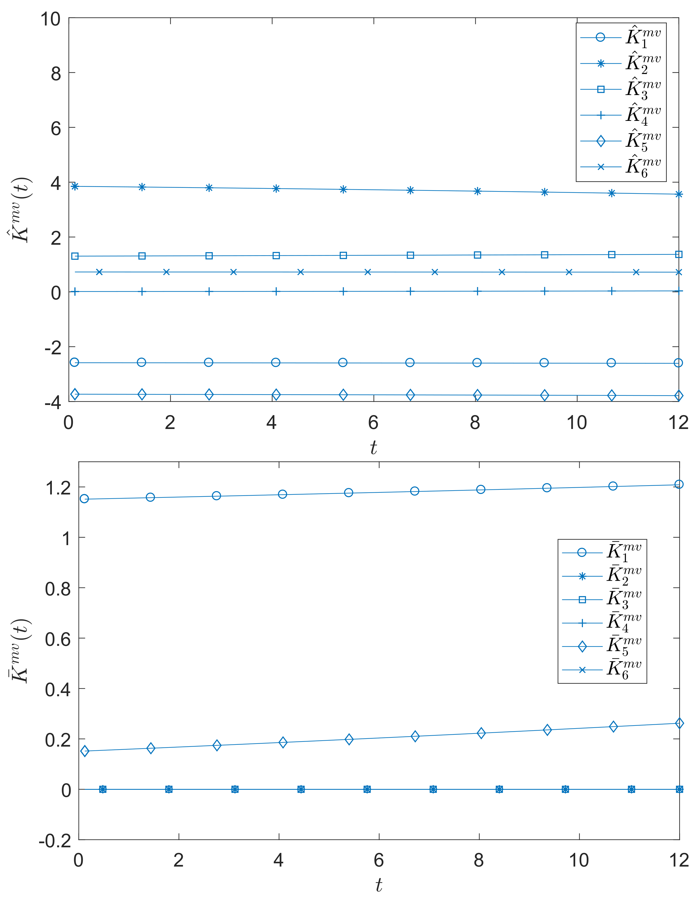
Based on Theorem 1, we can compute the optimal Lagrangian multiplier as , and the optimal portfolio policy is
where and are plotted in Figure 1 for .
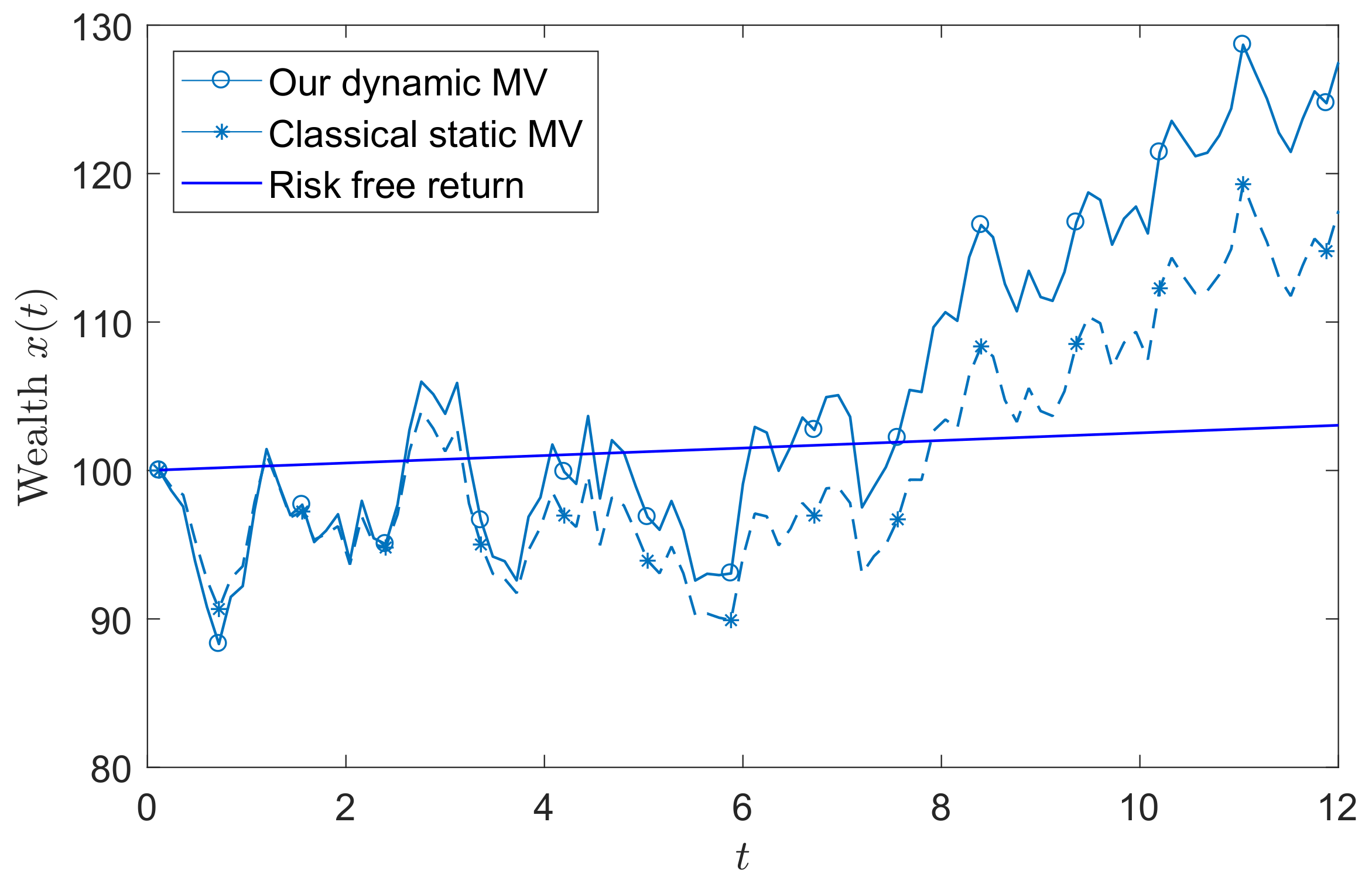
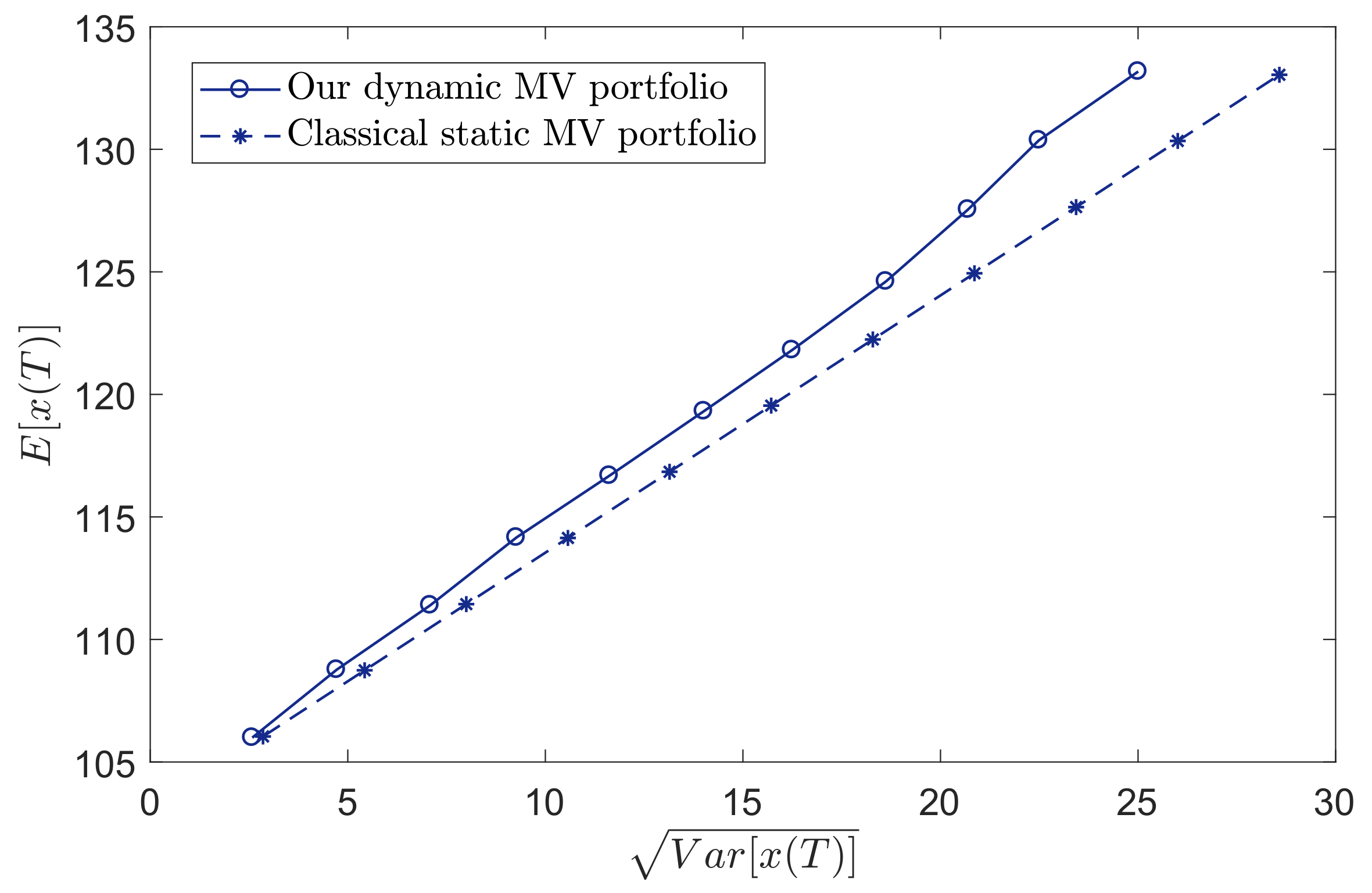
We used the buy-and-hold portfolio policy as a benchmark; i.e., we treated the total month as the one-period static MV portfolio selection model. All the constraints and parameters were set to be same as our dynamic MV portfolio selection model . Solving the problem provided us the buy-and-hold portfolio policy. Figure 2 plots the realizations of the wealth processes generated by our model and the static benchmark for the identical sample path of the price process. Figure 2 shows that our model performed better than the static benchmark model. To compare the performances of these two models, we plotted the mean-variance efficient frontier of the terminal wealth for two models in Figure 3. The efficient frontier describes the Parato optimal set of the mean and standard deviation of the wealth. In this example, the efficient frontier was plotted in the following way. We varied the expected terminal wealth level d and computed the correspondent optimal portfolio. Once we had the portfolio, we could compute the standard deviation of the terminal wealth. More specifically, we first simulated 100,000 sample paths for each return of risky assets, respectively. Then, we could compute the corresponding realized portfolio policy and realized terminal wealth. According to the realized terminal wealth, we could compute the expected value and standard deviation of terminal wealth. Figure 3 shows that our dynamic MV portfolio policy achieved a lower level of risk than the static MV portfolio policy for the same level of expected terminal wealth.
6. Conclusions
This paper revisited the dynamic MV portfolio selection problem with cone constraints in continuous-time. By reformulating our dynamic MV portfolio selection model into a special stochastic LQ optimal control model, we successfully developed the optimal portfolio policy for our model. Moreover, we provided an alternative method to resolve this dynamic MV portfolio selection problem with cone constraints. More specifically, instead of solving the correspondent HJB equation directly, we developed the optimal solution for this problem by using the special properties of value function induced from its model structure, such as the monotonicity and convexity of value function. This alternative method offers a new way of thinking under the constrained mean-risk framework and can be extended to solve another portfolio selection models with cone constraints. Finally, our illustrative example demonstrated that our dynamic MV portfolio policy dominates the static MV portfolio policy. For example, our dynamic MV portfolio policy achieved a lower level of risk than the static MV portfolio policy for the same level of expected terminal wealth. Moreover, our model performed better than the static benchmark model in terms of the realized wealth processes.
One possible future study will be to extend our results to the stochastic control problem with partial moments as the objective function, which has various applications in portfolio management, such as the mean-downside-risk portfolio optimization model. Moreover, it would also be significant to extend our results to the dynamic portfolio problem with no bankruptcy constraint and other trading constraints, such that our model becomes easier to be applied to real portfolio management.
Author Contributions
Data curation, L.W.; methodology, S.P.; writing—original draft preparation, W.W.; writing—review and editing, R.X. All authors have read and agreed to the published version of the manuscript.
Funding
This work was supported by the National Natural Science Foundation of China under grant 61573244, “Stochastic control optimization of uncertain systems based on offset with multiplicative noises and its applications in the financial optimization”.
Institutional Review Board Statement
Not applicable.
Informed Consent Statement
Not applicable.
Data Availability Statement
Not applicable.
Conflicts of Interest
The authors declare no conflict of interest.
Appendix A
Appendix A.1. The Proof of Lemma 1
Proof.
We first consider . Since is a feasible solution of , we obtain
Thus, it has ≥ which leads to the following inequality:
Similarly, we can prove that . Now, we show that
If =0, it has
which is contradict to the fact
according to expression (6) and under the Assumption 1. □
Appendix A.2. The Proof of Theorem 1
Proof.
By applying Theorem 2 in [18], we obtain the optimal policy of problem () for any fixed :
The remaining task is to identify the optimal Lagrangian multiplier . From Theorem 2 in [18], it not hard to derive the optimal value of problem for any fixed as
Then, the optimal Lagrangian multiplier can be identified by maximizing . According to (7) and (8), we can find that is a piece-wise concave function with respect to . Therefore, the optimal Lagrangian multiplier can be derived as (12). The optimal portfolio decision (9) can be achieved by replacing with in (A1). □
Appendix A.3. The Proof of Lemma 2
Proof.
Firstly, we will prove the convexity of the value function . Let and be any different admissible pairs. We define , for any . It is easily to verify that satisfies . That is to say, is an admissible pair. Therefore,
where the last inequality holds true due to the convexity of square function. Since and were chosen arbitrarily, we can find that
Therefore, the convexity of can be established.
Secondly, before we show that is strictly decreasing on and is strictly increasing on , we need show that the value function while . Indeed, we assume that . After that, we could obtain if taking . Therefore, we have
Based on the non-negative of square function, we could obtain the result that .
Finally, we will focus on proving is strictly increasing on , the other part is similar. For any , there exists k such that
where . Thus, based on the convexity of , we have
where the second inequality is from the fact that and the last inequality is according to the assumption that . This result implies that is strictly increasing in , which completes the proof.
□
Appendix A.4. The Proof of Theorem 3
Proof.
Combining Theorem 2 and Lemma 2, we could easily obtain the optimal solution for the HJB Equation (14) as follows:
where . Indeed, if we let , it has . However, this result conflicts with Lemma 2, since is strictly decreasing on and strictly increasing on , for each fixed .
Recall that if there are no strategy constraints, the optimal solution for the HJB Equation (14) is
Thus, if we define
it is not hard to see that solving the HJB Equation (14) is equivalent to solve the following auxiliary HJB equation without strategy constraints
More specifically, the solution of (A3) is equal to the one of (14). In fact, the solution to the HJB Equation (A3) is also the value function associated with the following problem:
This problem has been widely studied in the literature and can be solved by the stochastic optimal control or martingale method (see, [3,5]). The optimal portfolio policy of problem () is
Therefore, the optimal control of mean-variance problem with cone constraints is (15). □
References
- Markowitz, H.M. Portfolio Selection. J. Financ. 1952, 7, 1063–1070. [Google Scholar]
- Li, D.; Ng, W.L. Optimial dynamic portfolio selection: Multiperiod mean-variance formulation. Math. Financ. 2000, 10, 387–406. [Google Scholar] [CrossRef]
- Zhou, X.Y.; Li, D. Continuous-Time Mean-Variance Portfolio Selection: A Stochastic LQ Framework. Appl. Math. Optim. 2000, 42, 19–33. [Google Scholar] [CrossRef]
- Zhu, S.S.; Li, D.; Wang, S.Y. Risk control over bankruptcy in dynamic portfolio selection: A generalized mean-variance formulation. IEEE Trans. Autom. Control. 2004, 49, 447–457. [Google Scholar] [CrossRef]
- Bielecki, T.; Jin, H.Q.; Pliska, S.R.; Zhou, X.Y. Continuous-time mean-variance portolio selection with bankrupcy prohibition. Math. Financ. 2005, 15, 213–244. [Google Scholar] [CrossRef]
- He, X.D.; Zhou, X.Y. Dynamic portfolio choice when risk is measured by weighted VaR. Math. Oper. Res. 2015, 40, 773–796. [Google Scholar] [CrossRef] [Green Version]
- Gao, J.J.; Xiong, Y.; Li, D. Dynamic mean-risk portfolio selection with multiple risk measures in continuous-Time. Eur. J. Oper. Res. 2016, 249, 647–656. [Google Scholar] [CrossRef]
- Gao, J.J.; Zhou, K.; Li, D.; Cao, X.R. Dynamic mean-LPM and mean-CVaR portfolio optimization in continuous-time. SIAM J. Control. Optim. 2017, 55, 1377–1397. [Google Scholar] [CrossRef] [Green Version]
- Zhou, K.; Gao, J.J.; Li, D.; Cui, X.Y. Dynamic mean-VaR portfolio selection in continuous time. Quant. Financ. 2017, 17, 1631–1643. [Google Scholar] [CrossRef]
- Cui, X.Y.; Li, X.; Li, D. Unified framework of mean-field formulations for optimal multi-period mean-variance portfolio selection. IEEE Trans. Autom. Control. 2014, 59, 1833–1844. [Google Scholar] [CrossRef] [Green Version]
- Strub, M.S.; Li, D.; Cui, X.Y.; Gao, J.J. Discrete-time mean-CVaR portfolio selection and time-consistency induced term structure of the CVaR. J. Econ. Dyn. Control. 2019, 108, 103751. [Google Scholar] [CrossRef]
- Li, X.; Zhou, X.Y.; Lim, A.E.B. Dynamic mean-variance portfolio selection with no shorting constraints. SIAM J. Control. Optim. 2002, 40, 1540–1555. [Google Scholar] [CrossRef]
- Cui, X.Y.; Gao, J.J.; Li, X.; Li, D. Optimal multi-period mean-variance policy under no-shorting constraint. Eur. J. Oper. Res. 2014, 234, 459–468. [Google Scholar] [CrossRef]
- Gao, J.; Li, D.; Cui, X.; Wang, S. Time cardinality constrained mean-ariance dynamic portfolio selection and market timing: A stochastic control approach. Automatica 2015, 54, 91–99. [Google Scholar] [CrossRef]
- Wu, W.P.; Gao, J.J.; Li, D.; Shi, Y. Explicit Solution for Constrained Scalar-State Stochastic Linear-Quadratic Control with Multiplicative Noise. IEEE Trans. Autom. Control. 2019, 64, 1999–2012. [Google Scholar] [CrossRef]
- Cui, X.Y.; Li, D.; Li, X. Mean-variance policy for discrete-time cone constrained markets: The consistency in efficiency and minimum-variance signed supermartingale measure. Math. Financ. 2017, 27, 471–504. [Google Scholar] [CrossRef]
- Hu, Y.; Zhou, X.Y. Constrained stochastic LQ control with random coefficients, and application to portfolio selection. SIAM J. Control. Optim. 2005, 44, 444–466. [Google Scholar] [CrossRef]
- Wu, W.P.; Gao, J.J.; Lu, J.G.; Li, X. On continuous-time constrained stochastic linear–quadratic control. Automatica 2020, 114, 108809. [Google Scholar] [CrossRef]
- Pham, H. Continuous-Time Stochastic Control and Optimization with Financial Applications; Springer: Berlin/Heidelberg, Germany, 2009. [Google Scholar]
- Yong, J.M.; Zhou, X.Y. Stochastic Controls: Hamiltonian Systems and HJB Equations; Springer: Berlin/Heidelberg, Germany, 1999. [Google Scholar]
Figure 1.
The outputs of and .

Figure 2.
The realized wealth processes.

Figure 3.
The efficient frontiers.

Publisher’s Note: MDPI stays neutral with regard to jurisdictional claims in published maps and institutional affiliations. |
© 2021 by the authors. Licensee MDPI, Basel, Switzerland. This article is an open access article distributed under the terms and conditions of the Creative Commons Attribution (CC BY) license (https://creativecommons.org/licenses/by/4.0/).
Share and Cite
MDPI and ACS Style
Wu, W.; Wu, L.; Xue, R.; Pang, S. Constrained Dynamic Mean-Variance Portfolio Selection in Continuous-Time. Algorithms 2021, 14, 252. https://0-doi-org.brum.beds.ac.uk/10.3390/a14080252
AMA Style
Wu W, Wu L, Xue R, Pang S. Constrained Dynamic Mean-Variance Portfolio Selection in Continuous-Time. Algorithms. 2021; 14(8):252. https://0-doi-org.brum.beds.ac.uk/10.3390/a14080252
Chicago/Turabian StyleWu, Weiping, Lifen Wu, Ruobing Xue, and Shan Pang. 2021. "Constrained Dynamic Mean-Variance Portfolio Selection in Continuous-Time" Algorithms 14, no. 8: 252. https://0-doi-org.brum.beds.ac.uk/10.3390/a14080252
Note that from the first issue of 2016, this journal uses article numbers instead of page numbers. See further details here.