1. Introduction
In order to have a better function of vibration isolation, support and limit, the mount needs to exhibit large stiffness and damping at low frequency to attenuate the large amplitude vibration. When excited at high frequency, it needs to exhibit small stiffness and damping to effectively isolate small amplitude vibration to get low noise level.
Since 1920 [
1], rubber mount had been used for vibration isolation of automotive powertrain. However, there are some issues such as insufficient damping at low frequency and large stiffness at high frequency.
Passive hydraulic engine mounts (HEMs) have experienced three generations of evolution: from the HEMs with orifice or inertia track (IT), to the HEMs with IT and decoupling membrane (DM) or decoupling disk, then to the HEMs with IT, DM and disturbing disk (DD). While maintaining large damping at low frequency, it has realized low stiffness and small damping at high frequencies [
2,
3], which brings the passive mount performance to their upper limits.
In recent years, automobile lightweight has gradually become a development trend. The significant increase in engine power density, the adoption of variable displacement engine (VDE) for improving fuel economy, and new requirements to further improve dynamic comfort, traditional passive mount cannot meet the increasingly stringent requirements of vibration isolation. In this way, semiactive control mounts are gradually receiving attention from the automotive industry researchers. A semiactive hydraulic mount based on two-state control of the solenoid valve ON and OFF can optimize the low-frequency and high-frequency dynamic characteristics, respectively [
4], but that only two states being adjustable limits its performance. Correspondingly, the vibration isolation performance of the active control mount (ACM) has been greatly improved [
5]. The ACM control algorithms play a decisive role in its performance. Different researchers often use different control algorithms [
6]. Roman et al. designed a piezoelectric ACM, the actuator is in no need of bearing static load; the test showed that through the series arrangement, the ACM could significantly reduce the second-order vibration excitation [
7]. Audi designed an electromagnetic ACM to solve the vibration problem caused by the V8 engine with only four cylinders operating under low load [
8]. Choi et al. proposed a linear oscillatory actuator applied to ACM, which has the characteristics of small permanent magnet and large output power. Simulations have verified the effectiveness of the designed actuator and control strategy [
9]. Priyandoko et al. used an adaptive control method to improve the performance index of the suspension system [
10]. Sharkawy et al. proposed fuzzy and adaptive fuzzy active suspension control strategies, and compared them with LQR, showing that the former had better control effects on providing smooth vertical motion [
11]. Hillis designed a F
xLMS controller for a four-cylinder turbo diesel engine, and evaluated the steady-state and transient performance of the ACM system through experiments, discovering that the chassis vibration was significantly reduced [
12].
In summary, the current related technologies for ACM are still not mature enough, their vibration isolation effect needs to be enhanced and their applications are not extensive enough in the meantime. Therefore, it is of great significance to carry out related research based on ACM. Compared with other types of ACM, electromagnetic ACM has the advantages of compact structure and stable performance. Therefore, this paper chooses an active control mount with an oscillating coil actuator as the research object. In addition, many experts and scholars have done related research on the control algorithms of ACM system, but most of them only apply one or several control algorithms to ACM. While this paper focuses on explore the feasibility of control algorithms applied to ACM systems and lay the foundation for controller and product development.
In this paper, based on the ACM lumped parameter model (LPM), nine different control algorithms, including least mean-square (LMS) adaptive feedforward control, recursive least square (RLS) adaptive feedforward control, filtered reference signal LMS (FxLMS) adaptive control, linear quadratic regulator (LQR) optimal control, H2 control, H∞ control, proportional integral derivative (PID) feedback control, fuzzy control and fuzzy PID control, are used to simulate the system and analyse their vibration isolation performance, and an optimal control algorithm can be selected for ACM.
2. Modelling of ACM
The ACM model, including the electromagnetic actuator model, is build based on the passive hydraulic mount model. In order to simplify the model, the following assumptions are made: (1) the fluid in the mount is incompressible, (2) the pressure distribution in the upper and lower fluid chambers is uniform, (3) the fluid in the upper and lower chambers is leak-free, (4) the fluid does laminar flow in the inertia track.
The output force of the electromagnetic actuator in the ACM is linear with the input current between 25 Hz and 250 Hz, while the excitation frequency of the four-cylinder four-stroke in-line engine is generally 25~200 Hz [
13]. In this way, the actuator is suitable for the application in ACM.
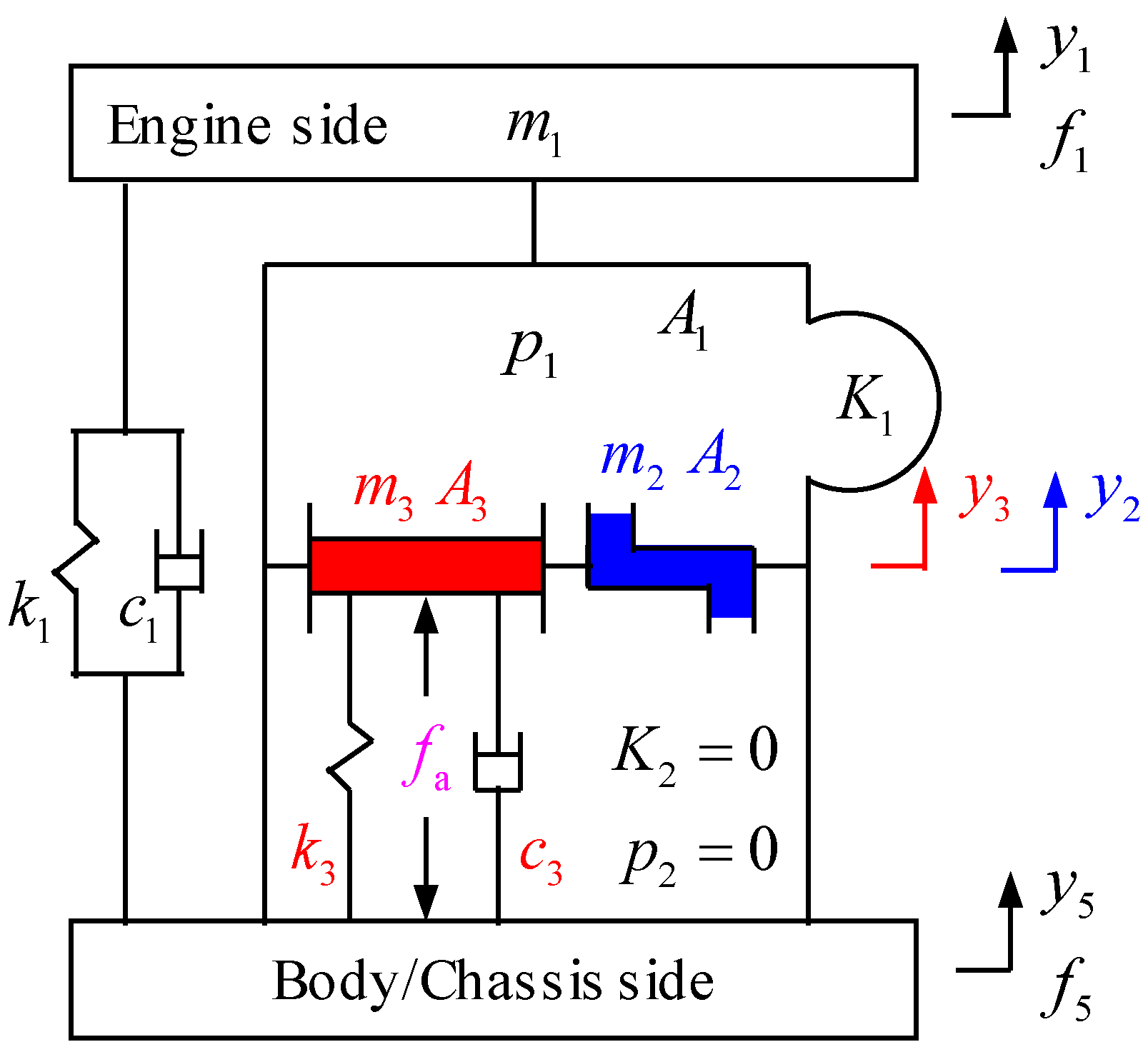
The ACM mechanical model is established as shown in
Figure 1, it is stipulated that upward is the positive direction. The meaning of each parameter and the corresponding values are shown in
Table 1. The excitation displacement at engine side is
y1(
t) and it is assumed that the chassis side degree of freedom
y5(
t) is fixed, that is
y5(
t) = 0. The forces applied to the engine side and transmitted to the chassis side are
f1(
t) and
f5(
t), respectively. The displacement of the fluid in inertia track and the DM are
y2(
t) and
y3(
t), respectively. The relative pressures of the upper and lower chambers are
p1(
t) and
p2(
t), respectively. Since the bulk stiffness of the rubber bellow,
K2, is about zero due to the crimpled lower rubber bellow, set
p2(
t) = 0. The
fa(
t) is the active force of electromagnetic actuator. According to the ACM mechanical model shown in
Figure 1, the ACM mathematical model can be derived as Equation (1) [
3,
14,
15].
3. Design of ACM Controller
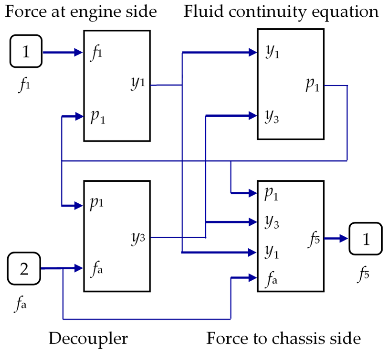
When the frequency is higher than the resonance frequency of the fluid channel, the inertia track is nearly closed due to the increase of fluid resistance. Thus, the movement of the inertia liquid column can be ignored and
y2 = 0. The mathematical model of ACM system of
Section 2 is approximately equivalent to linear model. Based on the ACM mathematical model, the simulation model of the ACM can be established in MATLAB/Simulink, as shown in
Figure 2.
In order to evaluate the control performance of different control algorithms and select the most appropriate control algorithm, the ACM controller is added to the simulation model [
16].
3.1. LMS Adaptive Feedforward Control
The adaptive process of adaptive filter is essentially the process of finding the optimal weight vector
w(
n) in an iterative manner. The optimization methods include LMS, RLS, transform domain adaptive filtering algorithm and related algorithms derived from these. The LMS algorithm has the advantages of simple structure, easy implementation by hardware, and strong robustness. Construct a simulation environment with random disturbances, as shown in
Figure 3.
The LMS algorithm is based on the method of steepest descent, which is a stochastic implementation of the steepest descent method. It is derived on the basis of minimizing the instantaneous mean square error with adaptive weight coefficients recursively updated, moving
w(
n) in proportion to the instantaneous gradient estimate of the mean-square error [
17,
18,
19].
The error signal
e(
n) is the difference between the desired output
d(
n) and the actual output
y(
n) of the filter at time
n, namely,
Because LMS adaptive feedforward control has strong robustness and anti-random disturbance, random disturbance
r(
n) is introduced. The performance function
ξ is defined as the mathematical expectation of the square value of the error signal
e(
n), namely:
Therefore, the adaptive filter can be expressed as:
Finding the optimal weight
w(
n) to minimize
ξ(
n).
w(
n) can be recursively updated at every sample time by an amount proportional to the negative instantaneous value of the gradient, a modified form of the well-known LMS algorithm is produced as below.
where
μ is a parameter named convergence factor that affects the stability and convergence of algorithm, and ∇(
n) is the mean-square error gradient. In practical applications, in order to simplify the calculation and meet the real-time requirements, the gradient
of the instantaneous square error
e2(
n) of a single error sample is generally taken as an estimate of the mean-square error gradient, it can be expressed as:
Thus, the iterative update formula of the weight
w(
n) is as follows:
The correction term of the iterative update formula of traditional LMS algorithm weight
w(
n) is proportional to the size of the input reference signal
x(
n). It will encounter the problem of noise gradient amplification under the circumstance of the value of
x(
n) is large. In order to solve this problem, the iterative update formula of the weight
w(
n) is transformed as below.
By introducing the square term of the Euclidean norm of x(n), the correction term of the weight coefficient iterative update formula is normalized by it, where γ is a parameter named correction factor that avoids the value of is too small to cause the correction term to be too large, which makes numerical calculation difficult.
In this way, the algorithm process of LMS can be expressed by the following formula:
The convergence of LMS algorithm depends on convergence coefficient μ. As long as the value of μ is between 0 and the reciprocal of the maximum eigenvalue of the input autocorrelation matrix E{x(n)xT(n)}, the convergence of the algorithm can be guaranteed from any initial weight, that is, the weight w converges to the optimal value to minimize the error.
The simulation model of the LMS algorithm is established in MATLAB/Simulink. A swept frequency signal is used to simulate the excitation force at engine side, and a random disturbance is added to ACM system to reflect the robustness of LMS algorithm.
3.2. RLS Adaptive Feedforward Control
The RLS algorithm is a recursive least square algorithm [
20], which implements an exact least square solution by recursive. The control block diagram is similar to
Figure 3. Compared with LMS, RLS algorithm has poor tracking ability in non-stationary environment, complicated calculation and is difficult to implement, but it has the characteristic of fast convergence.
In order to avoid the existence of instability problems, the error function minimized in RLS algorithm is generally defined as the exponential weighted sum of squared errors:
where
β ≤ 1, it is a positive constant named forgetting factor, generally a value close to 1 being chosen;
ei is the residual signal (error signal) at time
i. At time
k, the least square algorithm yields the optimal estimate of the weight vector
wk in the sense of least squares is below: for
is:
where the recurrence formula of
Rk and
Pk is shown below:
Let
,
,
,
. For a matrix
A in the form
, according to the matrix inversion lemma, its inverse is
. Applying the matrix inverse lemma to Equation (12) to obtain Equation (14):
where
Kk is the gain vector and the expression is:
let
Gk =
, it can be expressed as:
and we find there exist Equation (17) as below:
Apply the above formula, Equations (13), (16) and (17) are introduced into Equation (11). After algebraic processing, the weight coefficient update formula is obtained:
where
.
The above equations summarize this algorithm, when matrix is initialized to , where δ−1 is a small positive constant, I is an unit matrix, and the weight coefficients are simply initialized to zero.
In MATLAB/Simulink, the DSP toolbox is used to build the simulation model of RLS algorithm. It can be seen in the oscilloscope that the RLS algorithm is in good convergence behaviour.
3.3. FxLMS Adaptive Control
F
xLMS algorithm is the most popular adaptive control algorithm in the field of active noise control (ANC) and active vibration control (AVC). It is derived from LMS algorithm, and the concept of “filtered-
x” was proposed firstly by [
21]. In one of the landmark papers in the development of ANC, Elliott et al. [
22] firmly established the “F
xLMS” terminology as a cornerstone in that field. A closely related usage of the F
xLMS algorithm is in the area of AVC [
23], which has many applications in reducing mechanical vibrations from all sorts of machinery as well as naturally occurring seismic vibrations. Again, as in acoustic applications, it has remarkable noise reduction capability in low frequency band.
F
xLMS is an improvement of LMS algorithm, which ameliorate the situation that LMS algorithm cannot handle the vibration and noise reduction of narrow frequency bands well. The essential difference between F
xLMS and LMS is that the secondary path is added to filter the reference signal, which is one of the factors determining the performance of F
xLMS [
24]. In order to compensate for the dynamics of the secondary path
S(
z), the reference signal has to be filtered with a secondary path estimate
[
15]. The F
xLMS algorithm is simple, easy to implement, and has good stability, which is conducive to constructing a simulation environment with random disturbances.
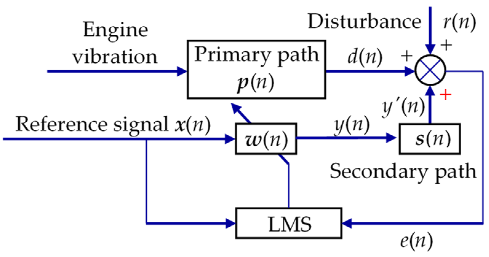
Figure 4 is a schematic diagram of F
xLMS algorithm. The vibration
d(
n) at the chassis, which is to be cancelled, results from the engine vibration
v(
n) transmitted through the passive dynamic characteristics
P(
z) of the ACM represented by its impulse response
p(
n). The
y(
n) is the control output of the adaptive filter,
y′(
n) is the second path output. The error signal
e(
n) measured at the chassis side is the sum of source vibration signal
d(
n) and active anti-vibration signal
y′(
n) generated by the controlled actuator.
At time
n, the output
y(
n) of the
Ith-order finite impulse response (FIR) control filter is equal to the convolution operation [
25]:
where
x(
n) is the reference signal. The transfer function of the secondary path can be simulated by using an
Jth-order FIR filter
S(
z) in time domain.
s(
n) = [
s0,
s1…
sj…
sJ−1]
T is the impulse response sequence,
is the estimated
s(
n) for secondary path. The active anti-vibration
y′(
n) produced by the control path is equal to the convolution of the control output of LMS filter and the secondary path transfer function:
The gradient descent algorithm used to adjust the weights in the source FIR filter is:
where
x′(
n) is the filtered reference signal vector:
Equation (22) is the weight iterative derivation formula of F
xLMS algorithm [
22]. When simulating in MATLAB/Simulink, taking into account the characteristics of engine excitation, the convergence coefficient
μ needs to be appropriately increased into 0.1 to speed up the algorithm convergence at low speeds, while decreased to be 0.05 to maintain the stability of the algorithm at high speeds.
The assumption of time invariance in the filter coefficients is equivalent, in practice, to assuming that the filter coefficients wi change only slowly compared to the timescale of the response of the system to be controlled. This timescale is defined by the values of the coefficients .
3.4. LQR Optimal Control
The control object of the LQR algorithm is a linear system given in the form of state space. Its objective function is a quadratic function with input object state and control input [
26]. The advantage of LQR algorithm lies in the fact that according to the variables to be optimized in the actual model, while taking into account the system performance and control energy, the optimal control law of stabilized linear feedback is obtained, which is easy to form a closed-loop optimal control, so that the comprehensive performance of the system is optimized.
The linear mathematical model of ACM system of
Section 2 is converted into the form of state equation and output equation.
The engine vibration
u1, control input variable
u2, state variable
x and output variable
y are as below:
In addition, we can get the state equation and the output equation
,
. Details as follows:
The goal of active control is to minimize the force transmitted to the chassis while ensuring that the engine side displacement and active force are not too great. Therefore, the objective function can be expressed as:
where
q and
r are weighting coefficient, and their values are determined according to different requirements of the ACM performance index. When we set the state variable weighting matrix
Q = [
q], the control input variable weighting matrix
R = [
r], the objective function becomes
Furthermore,
y =
Cx +
Du2, set
Qn =
CTQC,
Nn =
CTQD,
Rn =
R +
DTQD, the objective function can be expressed as
Set the optimal control amount (t) = Kx, the feedback matrix can be expressed as, K = −R( + BTP), P is the solution of Riccati equation ATP + PA − (PB + Nn)(BTP + ) + Qn = 0. When solving the Riccati equation, there is usually more than one solution that fits the equation itself, while there is only one symmetric positive definite solution which makes the system asymptotically stable and satisfies the condition of constructing the optimal state feedback gain matrix.
The LQR optimal control function is only related to A, B, Q, R, where A, B are known, the performance of the system depends on the values of the weighting matrices Q, R. Set R to be the identity matrix. After repeated debugging, Qn is a second-order unit matrix in this paper. When Q = 800, the system performance is the best, the optimal control matrix K can be obtained.
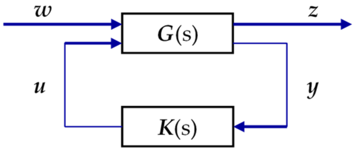
3.5. H2 and H∞ Control
In order to facilitate the use of H
2 and H
∞ control algorithms for various control problems, a general control block diagram is used, as shown in
Figure 5 [
27].
The control block diagram can be described as:
where
G(s) is the transfer matrix of the controlled object,
K(s) is the controller.
The state-space form of the controlled object
G can be presented as:
where
x is the state vector of the plant,
w is the input variable which represents all exogenous signals,
z is the output performance variable,
u is the control variable,
y is the measured output signal, the variable
u and
y are the output and input of the controller to be designed, respectively. The goal of control design is to minimize
z.
Using the following closed-loop transfer matrix to represent the input
w and output
z relationship.
The controller
K(
s) of the controlled system is designed to meet the performance index [
28]:
(H
2 control) or
(H
∞ control).
For the H
∞ (H
2) controller of the ACM, selecting the state variable:
. To see the performance of the ACM and the controller, selecting the output performance variable
z = [
f5 0.1
i]
T, measured output variable
y =
f5, and selecting active current as a control variable
u =
i. Input variable can be expressed as:
w =
f1. The equation of state is the same as Equation (25), the measured output equation is the same as Equation (26), and the output equation is thus obtained:
For a given controlled object ACM system, the output feedback controller
K which makes the closed-loop system stable and minimum ‖
Tzw(
s)‖
∞ can be solved by corresponding Riccati equation [
29].
MATLAB can be used to solve the Riccati equation and calculate the output feedback controller K, which is the solution of the H∞ controller. Similarly, the solution of the H2 controller can be obtained.
3.6. PID Feedback Control
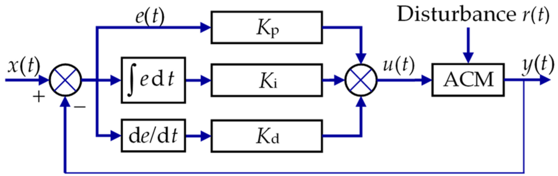
The PID controller is a linear feedback controller. It combines proportional, integral and derivative to form a control variable through linear combination, and controls the object. The function of the proportional link, integral link and differential link is to quickly reduce errors, eliminate steady-state errors and pre-judge the output to reduce overshoot, respectively. PID feedback control block diagram is shown in
Figure 6. The control law can be expressed as [
30]:
where
e(
t) =
x(
t) −
y(
t) is the error,
x(
t) is the desired reference signal, and the force desired to be transmitted to the body side is zero,
y(
t) is the measured output, and
r(
t) is the external random disturbance, the
Kp,
Ki and
Kd is the proportional, integral and differential coefficient, respectively.
The conventional PID control principle is simple, easy to use and robust. PID controller is a correction device that can change the original frequency domain characteristics of the system. Therefore, according to the system characteristics of ACM, set the frequency domain performance indicators desired by the system: amplitude crossover frequency and phase margin, and then the three parameters of the PID controller can be determined.
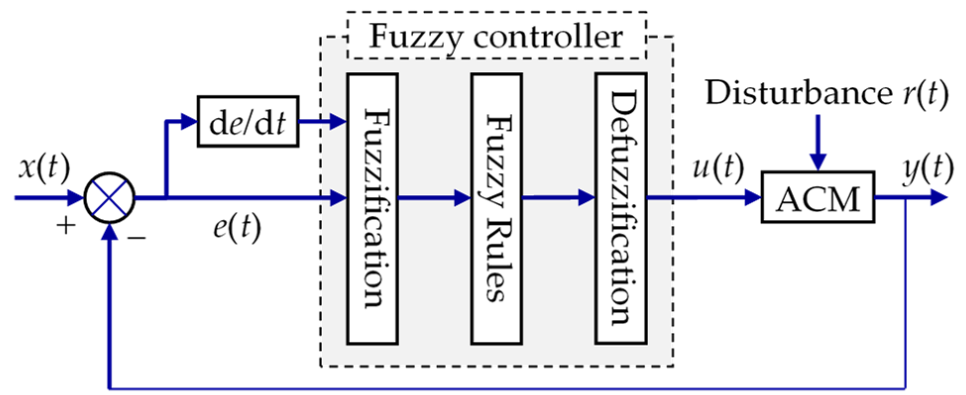
3.7. Fuzzy Control
The goal of an ACM system is to minimize or zero the force transmitted through the ACM to chassis. The fuzzy control design is simple, easy to apply, and robust [
31]. The input of the fuzzy controller is the error
e(
t) between the desired minimum transmitted force and the actual transmitted force and the change rate of the difference d
e(
t). The output
u(
t) of the fuzzy controller is the current acting on the actuator, which is then converted into active control force, and its composition is shown in
Figure 7.
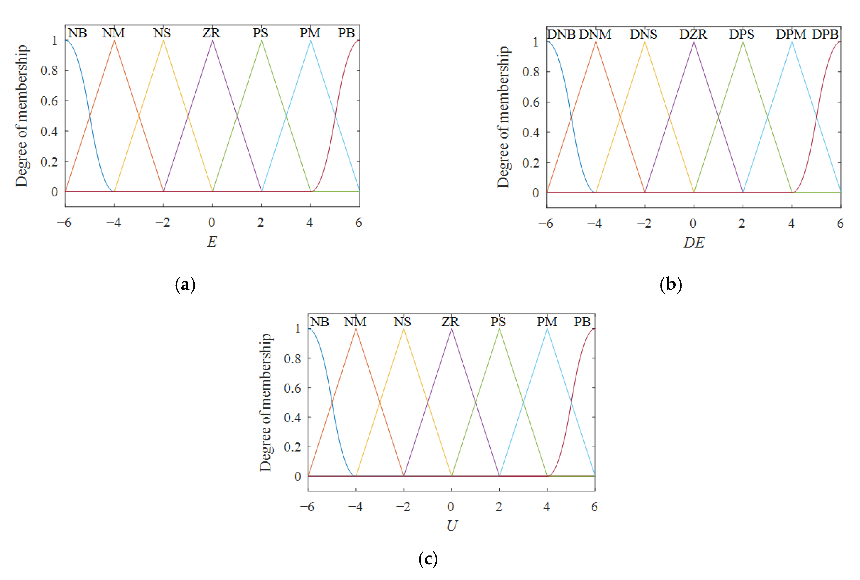
E,
DE and
U are used to denote the fuzzy sets of variables
e(
t), d
e(
t) and
u(
t), respectively. The domain of the input fuzzy sets
E and
DE are all normalized to {−6, −4, −2, 0, 2, 4, 6}, and the corresponding fuzzy subset is {negative big, negative middle, negative small, zero, positive small, positive middle, positive big} denoted as {NB, NM, NS, ZR, PS, PM, PB}, {DNB, DNM, DNS, DZR, DPS, DPM, DPB}, respectively. In order to reduce the structural complexity of the fuzzy controller and increase the calculation speed, the fuzzy subsets on the left and right sides use Z-type and S-type membership functions respectively, and the rest of the fuzzy subsets use triangular membership functions. The distribution method of membership functions is adopted evenly distributed. The membership functions are shown in
Figure 8a,b. The domain of the output fuzzy set
U is normalized to {−6, −4, −2, 0, 2, 4, 6}, and the corresponding fuzzy subset is the same as
E, membership function is shown in
Figure 8c.
The fuzzy control rules for the ACM control system are obtained from experience. The essence is to formulate the output of the fuzzy controller according to the different conditions of
E and
DE. When
E and
DE have the same signs, it means that the system output is far away from the reference signal. The main task of formulating the control variable
U should be to eliminate the error as soon as possible; when
E and
DE have opposite signs, it means that the system output is close to the reference signal. As the distance between the system output and the reference signal changes from large to small, the control variable
U is formulated to change from quickly eliminating errors to preventing overshoot. The fuzzy control rules as shown in
Table 2.
The function of the quantization factor (ke, kde) and the scale factor (ku) is equivalent to the external interface of the fuzzy controller. The function of the quantization factor is to map any input quantity to a fixed and finite interval, that is, the fuzzy domain. The function of the scale factor is to convert the value on the fuzzy domain into a value that can directly act on the controlled system. Use the trial-and-error method to determine the value of quantization factor and scale factor.
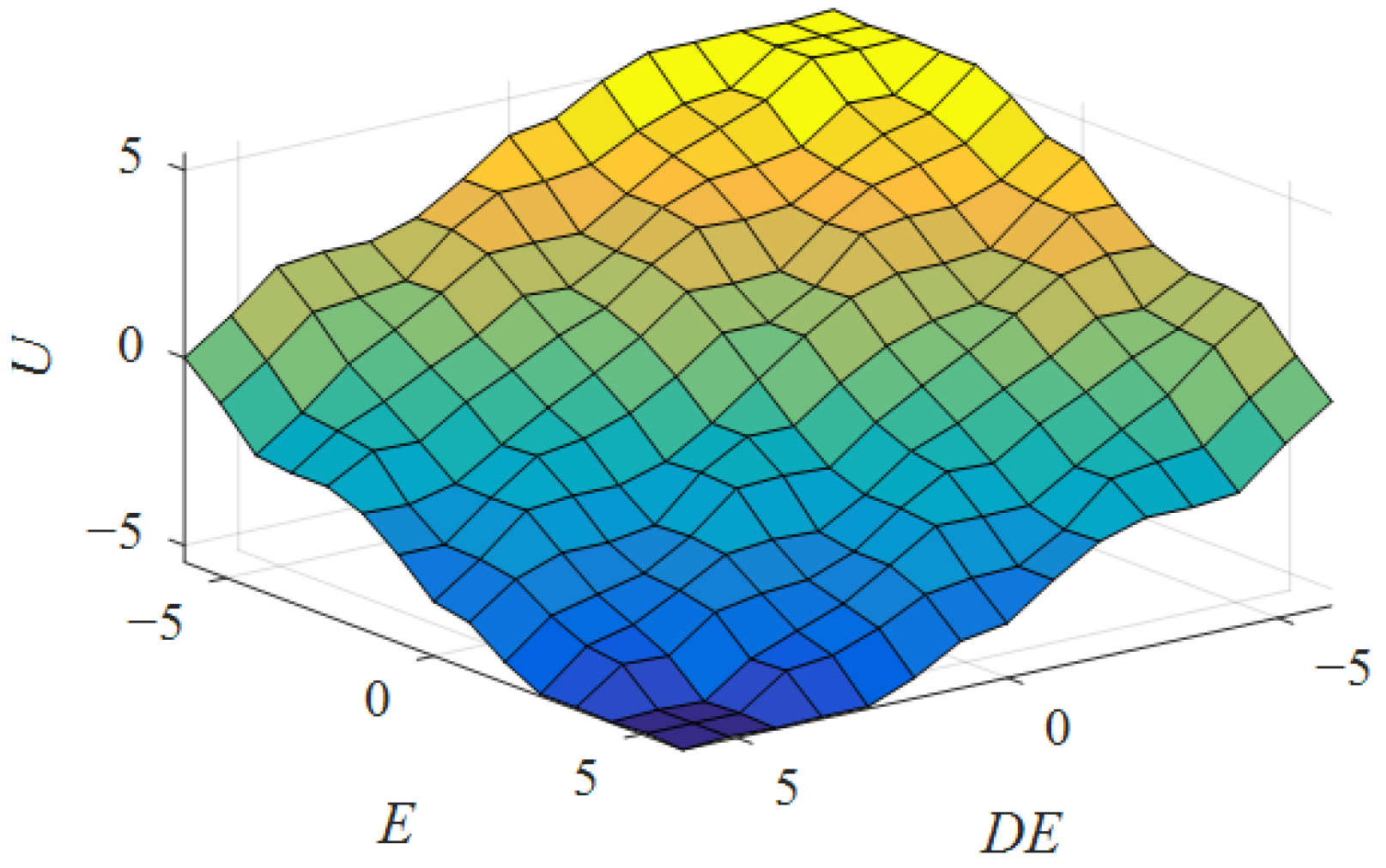
The Mamdani’s maximum-minimum reasoning method is applied. The area centre method, which is commonly used in engineering, is used to decompose the fuzzy problem. The input–output relationship of fuzzy controller is shown in
Figure 9. It is a smooth surface, which shows that the fuzzy control system has good robustness and stability. The fuzzy control simulation is carried out by using the fuzzy toolbox of MATLAB.
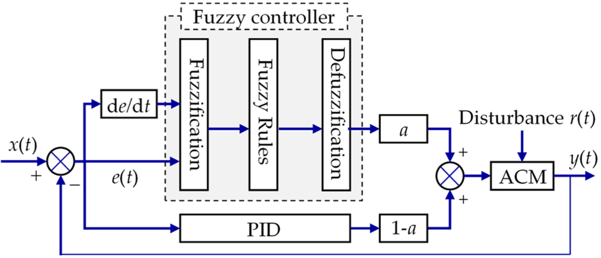
3.8. Fuzzy PID Control
Fuzzy PID control mainly involves two aspects [
32]. One is the hybrid structure of the fuzzy controller and the conventional PID, the other is the fuzzy self-tuning technique of the conventional PID parameters. In this section, the control block diagram of the hybrid fuzzy PID controller is shown in
Figure 10, and the control block diagram of the parameter self-tuning fuzzy PID controller is shown in
Figure 11.
Hybrid fuzzy PID control combines the advantages of fuzzy control and PID control, is easy to implement, and has strong robustness. The fuzzy controller is used in parallel with the PID controller to obtain a hybrid fuzzy PID controller. The fuzzy control is the same as that in
Section 3.7, and the PID control is the same as that
Section 3.6. The output of the controller is the sum of fuzzy controller and PID controller.
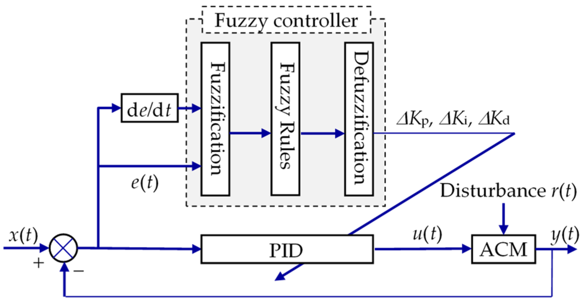
The basic idea of parameter self-tuning is to use fuzzy control rules to get the increment of PID control parameters, and add the increment to the initial value to realize real-time online adjustment of initial PID parameters. At this time, the three parameters of PID can be expressed as
Kp′,
Ki′ and
Kd′ are the values obtained by the method in
Section 3.6, and
kpu,
kiu and
kdu are the scale factors. Δ
Kp, Δ
Ki and Δ
Kd are the parameter increments obtained by fuzzy inference, and its fuzzy control rules as shown in
Table 3.
Parameter self-tuning fuzzy PID has the advantage of real-time adjustment of parameters, so it is chosen to represent the fuzzy controller.
In the MATLAB/Simulink, the fuzzy toolbox and the PID control toolbox are called to get the fuzzy PID control for simulation.
4. System Simulation and Comparison
MATLAB/Simulink is used to simulate the vibration characteristics of engine mount and the AVC performance of ACM controller. The simulation models of the nine active control algorithms above are established. In this study, the range of engine speed
n is 1000~6000 rpm. It is assumed that three mounts are used and the force
f1, i.e., the input of the model, is calculated by Equation (36):
where
Fe is vertical vibration force of the four-cylinder four-stroke in-line engine and
ω is angular velocity of the crankshaft and calculated by
ω = 2π
n/60. Other relevant parameters in the formula are shown in
Table 1.
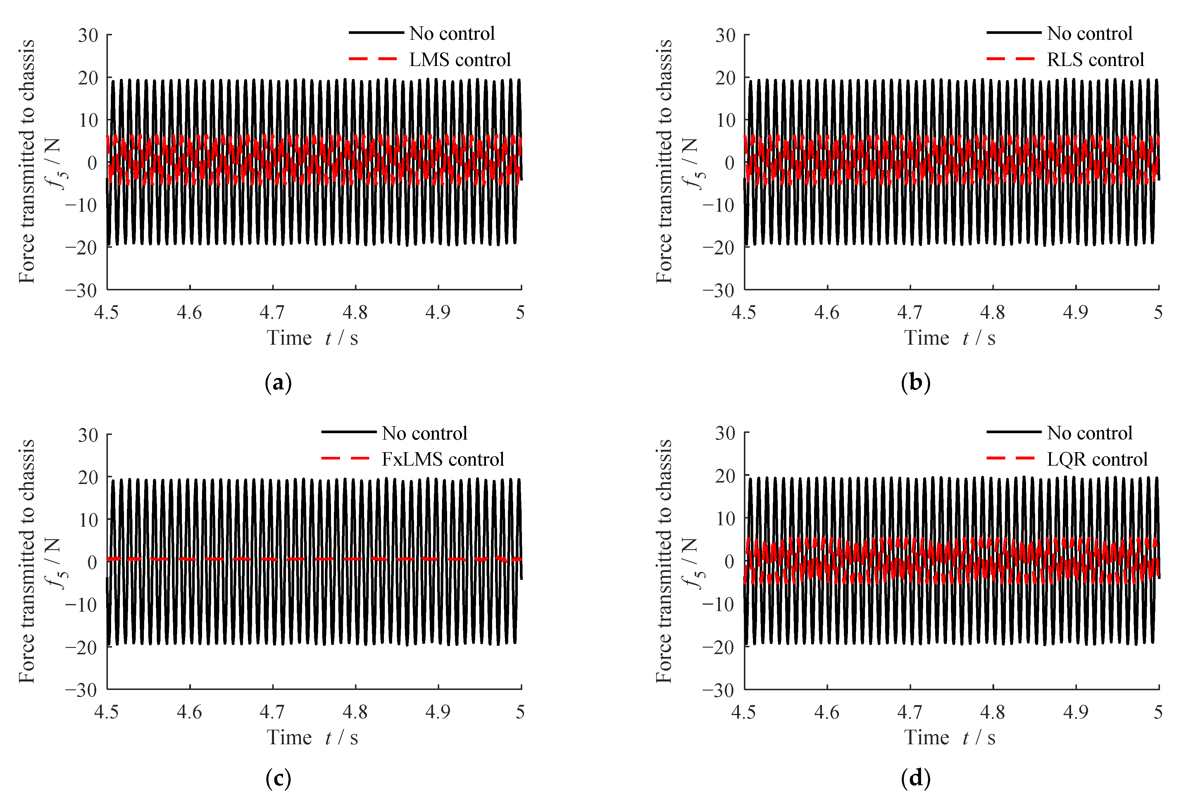
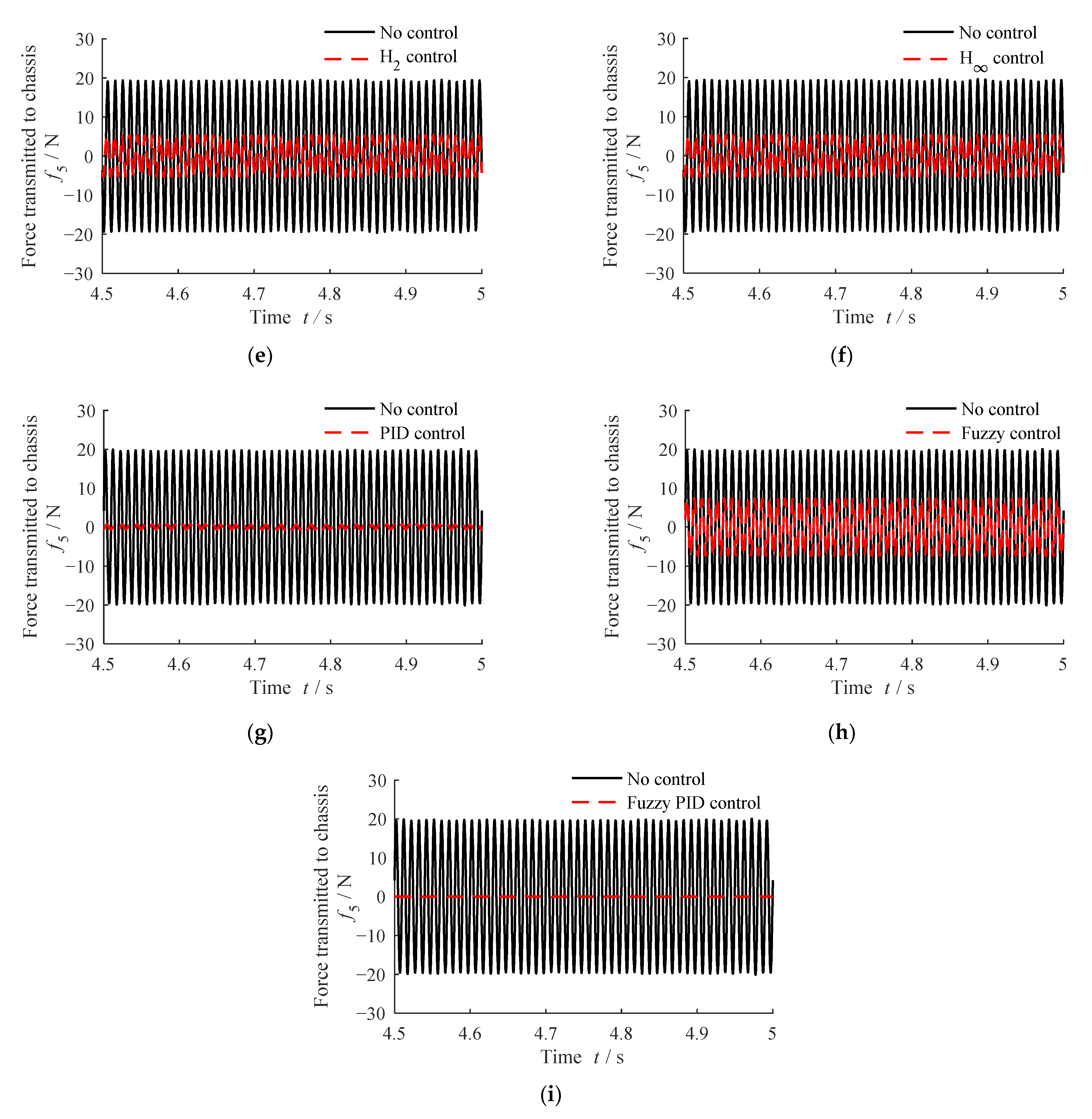
As shown in
Figure 12, the simulation results of time domain response of the force transmitted to the chassis side are obtained. Considering the engine speed at 3000 rpm, and the vibration in the vertical direction, with and without active control.
Figure 12a,b,d–f,h are simulations under the control of LMS, RLS, LQR, H
2, H
∞, and Fuzzy, respectively. The results show that the effectiveness of above control algorithms.
Figure 12c,g,i are simulations under the control of F
xLMS, PID, and Fuzzy PID algorithms, respectively. After controlling the current to drive the actuator to work, the force transmitted to the chassis side is greatly reduced compared to when there is no control.
In order to compare the active vibration isolation performance of nine control algorithms more intuitively, the force transmissibility is used to represent the vibration isolation performance of nine control algorithms and compared with the case of no control, as shown in
Table 4.
It can be seen from
Table 4 that the force transmissibility of ACM with nine control algorithms is much smaller than that without control.
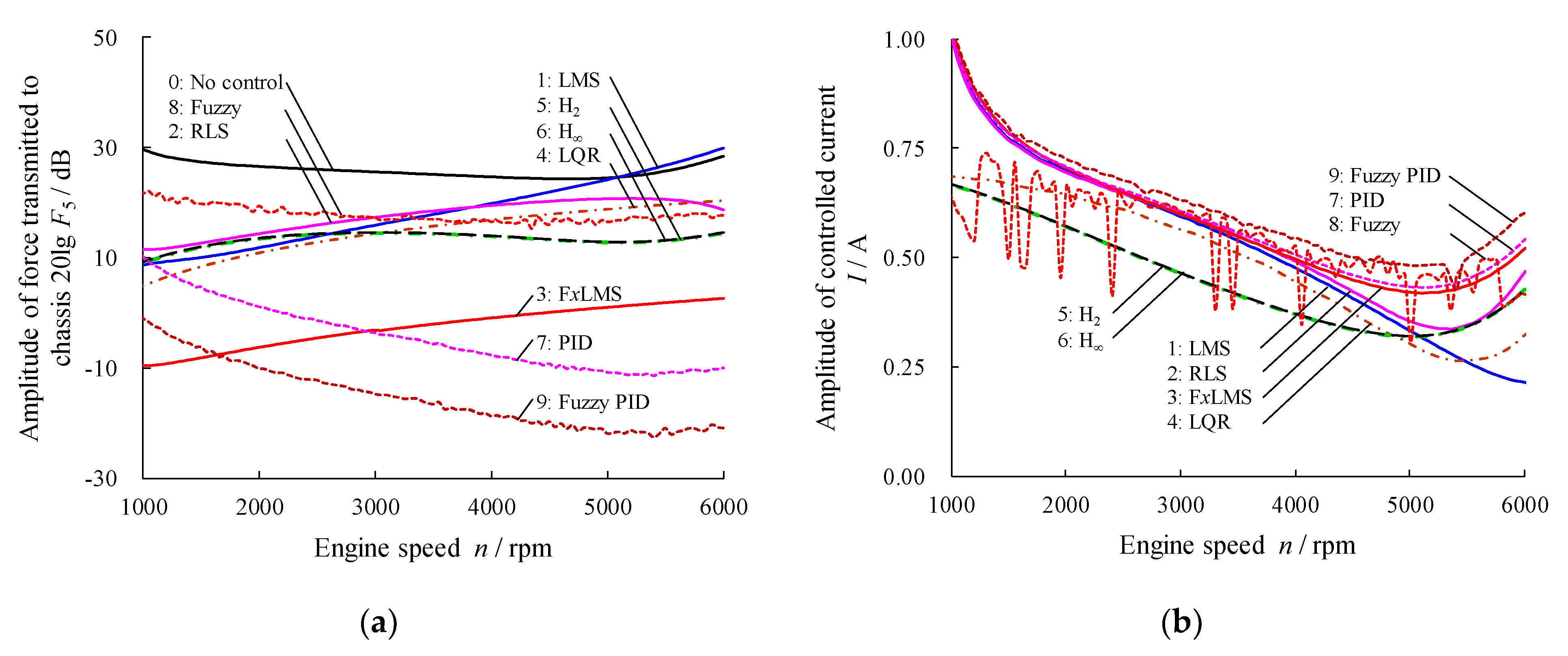
Figure 13a,b show the change of the force transmitted to the chassis and the controlled current at different engine speeds under nine active control algorithms, respectively. It could be seen that in the range of 1000~6000 rpm the force transmitted to the vehicle body after the control of eight algorithms except LMS is less than that before control. The control effect of LMS adaptive algorithm is effective at speeds below 5000 rpm and poor above 5000 rpm, and it is not even as good as passive engine mount. The reason lies in that LMS adaptive algorithm is extremely sensitive to phase errors, and excessive phase errors cause the algorithm to be unstable, which greatly reduces the control effect.
On the other hand, the results show that different algorithms have different control effects at different speeds. The LQR algorithm takes into account the system performance and control energy at the same time, so that the comprehensive index is optimized. Therefore, it may not be very prominent from the perspective of the vibration isolation effect. This characteristic is also reflected in the simulation results. However, compared with other algorithms, FxLMS, PID and Fuzzy PID control algorithms can reduce the force transmitted to the vehicle chassis more effectively in the range of 1000~6000 rpm, the force transmission is an order of magnitude lower than other control algorithms, and the control current at different speeds is also within a reasonable range. Meanwhile the PID controller is easily affected by the external environment in practical applications. Therefore, the advantages of PID applied to the ACM system that stimulates rapid changes are not prominent. The rules of the fuzzy PID controller need to be determined based on experience, the calculation is complicated and time-consuming. In addition, the scale factor and the quantization factor are determined by trial and error, which has a strong uncertainty, and needs to be debugged in practical applications. By contrast, the FxLMS adaptive control has the advantage of small amount of calculation, strong robustness and easy implementation by hardware. To sum up, the FxLMS adaptive control algorithm will be selected as the focus of further research about the active control algorithms of ACM.
5. Conclusions
Comparative research work of control algorithms for ACM is divided into three steps. Firstly, mechanical and mathematical models of ACM are established. Then, basing on the working principle of each control algorithm, the ACM controller is designed in the MATLAB/Simulink simulation environment. Finally, the simulation model of nine control algorithms for ACM are established to implement vibration isolation performance simulations for ACM.
For rotating machinery such as engines, FxLMS algorithm has been applied to the ACM system and the control effect has been obtained. This paper intends to study the feasibility and control effect of other algorithms in the ACM system. After experimental verification, it is possible to select several control algorithms that consume less computing resources to improve the economics of the product. The three control algorithms of LMS, RLS, and FxLMS all belong to feedforward control, and the relevant information of the disturbance source needs to be measured. The RLS algorithm has a large amount of calculation, while the FxLMS has a small amount of calculation, strong robustness and good control effect, which is suitable for the ACM system. The LQR, H2, and H∞ algorithms all have restrictions on the state space form, otherwise the controller cannot be solved, so some pre-processing of the state space model of the ACM system is required. PID algorithm can be applied to most systems, and its most important part is the adjustment of three parameters. The widely used empirical formula method, the Ziegler—Nichols method, as well as the critical oscillation method and damped oscillation method, are not suitable for this ACM system; therefore, three parameters are obtained by using frequency domain performance settings. Subsequent tests may be affected by the external environment, so fine-tuning will be made on this basis. Fuzzy control algorithms belong to the advanced control field, but the design of fuzzy rules requires prior knowledge and expert experience, and its structure is also relatively complex. Therefore, in actual application, it will be considered to be converted into an offline look-up table to reduce the calculation amount and running time of the controller.
The simulation results of different engine speeds from 1000 rpm to 6000 rpm show that except the LMS algorithm, the other eight algorithms have good control effect in the whole speed range, and the control current is in a reasonable range. FxLMS adaptive control algorithm, PID control algorithm and fuzzy PID control algorithm have the best vibration isolation performance among nine control algorithms. Furthermore, considering cost, implementation difficulty and stability, FxLMS adaptive control algorithm is more suitable for active control mount field than the fuzzy PID and PID control algorithms. Therefore, the FxLMS adaptive control algorithm can be selected and applied to ACM.
The active mounting system development process includes offline simulation, semi-physical simulation and full-physical simulation. In this paper, the offline simulations of nine control algorithms for the ACM system are studied. The latter simulation will be completed: semi-physical simulation (rapid control prototype, referred to as RCP), the control system is composed of a dSPACE simulation platform and a computer to complete the smooth transition from prototype controller to production controller; in full-physical simulation, the control system consists of a development board and computer composition, confirm the consistency of the functions completed by the controller and RCP. The experiments and verifications will be carried out in the next step, including bench test at MTS or Inova Elastomer Test System, bench test at powertrain-mounting system test, and vehicle test to verify the effectiveness of the control algorithms. It will lay a solid foundation for the development and realization of ACM.
Author Contributions
Conceptualization, R.-L.F.; Methodology, R.-L.F.; Software, R.-L.F., P.W., C.H., L.-J.W., Z.-J.L. and P.-J.Y.; Validation, P.W., C.H., L.-J.W., Z.-J.L. and P.-J.Y.; Formal analysis, R.-L.F.; Data curation, R.-L.F.; Writing—original draft preparation, P.W.; Writing—review and editing, R.-L.F., P.W., C.H., L.-J.W. and Z.-J.L.; Supervision, R.-L.F.; Project administration, R.-L.F. All authors have read and agreed to the published version of the manuscript.
Funding
This research was funded by the National Natural Science Foundation of China (No. 51175034) and the Scientific and Technological Innovation Foundation of Shunde Graduate School, USTB (No. BK19CE002).
Institutional Review Board Statement
Not applicable.
Informed Consent Statement
Not applicable.
Data Availability Statement
Not applicable.
Acknowledgments
We are grateful to Anhui Eastar Active Vibration Control Technology Co. Ltd. and Anhui Eastar Auto Parts Co. Ltd. for their financial support. We are also grateful to the National Natural Science Foundation of China (No. 51175034) and the Scientific and Technological Innovation Foundation of Shunde Graduate School, USTB (No. BK19CE002) for supporting this work.
Conflicts of Interest
The authors declare no conflict of interest.
References
- Zhang, C. Research and Optimum on Engine Rubber Mounts; Southeast University: Nanjing, China, 2006. [Google Scholar]
- Shi, W.; Lin, Y.; Lu, Z.; Feng, Z. A Study on Hydraulic Mounting Isolation Characteristics for Audi100 Car. J. Jilin Univ. Technol. 1996, 26, 10–15. [Google Scholar]
- Fan, R.L.; Lu, Z.H. Fixed points on the nonlinear dynamic properties of hydraulic engine mounts and parameter identification method: Experiment and theory. J. Sound Vib. 2007, 305, 703–727. [Google Scholar] [CrossRef]
- Fan, R.-L.; Zhang, X.-L. Study on Semi-active Hydraulic Mount with Variable-stiffness Decoupling Membrane. Chin. J. Automot. Eng. 2015, 51, 108–114. [Google Scholar] [CrossRef]
- Lee, Y.W.; Lee, C.W. Dynamic analysis and control of an active engine mount system. Proc. Inst. Mech. Eng. Part D J. Automob. Eng. 2002, 216, 921–931. [Google Scholar] [CrossRef]
- Han, Z.; Tian, X.; Dong, X. Swarm intelligent algorithm for re-entrant hybrid flow shop scheduling problems. Int. J. Simul. Process. Model. 2019, 14, 17–27. [Google Scholar] [CrossRef] [Green Version]
- Roman, K.; Sven, H.; Jonathan, M. Development of Active Engine Mounts Based on Piezo Actuators. ATZ Worldw. 2014, 116, 46–51. [Google Scholar]
- Rmling, S.; Vollmann, S.; Kolkhorst, T. Active Engine Mount System in the New Audi S8. MTZ Worldw. 2013, 74, 34–38. [Google Scholar] [CrossRef]
- Choi, I.; Hirata, K.; Niguchi, N. Design and Analysis of a Linear Oscillatory Actuator for Active Control Engine Mounts. In Linear Drives for Industry Applications (LDIA); The Institute of Electrical Engineers of Japan: Osaka, Japan, 2017. [Google Scholar]
- Priyandoko, G.; Mailah, M.; Jamaluddin, H. Vehicle active suspension system using skyhook adaptive neuro active force control. Mech. Syst. Signal Process. 2009, 23, 855–868. [Google Scholar] [CrossRef]
- Sharkawy, A.B. Fuzzy and adaptive fuzzy control for the automobiles’ active suspension system. Veh. Syst. Dyn. 2005, 43, 795–806. [Google Scholar] [CrossRef]
- Hillis, A.J. Multi-input multi-output control of an automotive active engine mounting system. Proc. Inst. Mech. Eng. Part D J. Automob. Eng. 2011, 225, 1492–1504. [Google Scholar] [CrossRef]
- Chen, S. The Design and Characteristic Simulation of Electromagnetic Hydraulic Mount; Jilin University: Changchun, China, 2007. [Google Scholar]
- Lee, B.H.; Lee, C.W. Model based feed-forward control of electromagnetic type active control engine-mount system. J. Sound Vib. 2009, 323, 574–593. [Google Scholar] [CrossRef]
- Hausberg, F.; Scheiblegger, C.; Pfeffer, P. Experimental and analytical study of secondary path variations in active engine mounts. J. Sound Vib. 2015, 340, 22–38. [Google Scholar] [CrossRef]
- Zhang, Y.; Tang, T.; Zheng, W. A train control system simulation and analysis method. Int. J. Simul. Process. Model. 2012, 7, 57–66. [Google Scholar] [CrossRef]
- Widrow, B.; Hoff, M.E. Adaptive switching circuits. Solid-State Electronics Laboratory, Stanford Electronics Laboratories. In Technical Report No. 1553–1; Stanford University: Stanford, CA, USA, 1960. [Google Scholar]
- Widrow, B. Adaptive filters. Asp. Netw. Syst. Theory 1971, 687, 653. [Google Scholar]
- Widrow, B.; McCool, J.; Ball, M. The complex LMS algorithm. Proc. IEEE 1975, 63, 719–720. [Google Scholar] [CrossRef]
- Xue, D. Computer Aided Control Systems Design Using MATLAB Language, 2nd ed.; TsingHua University Press: Beijing, China, 2006. [Google Scholar]
- Widrow, B.; Shur, D.; Shaffer, S. On adaptive inverse control. Proceeding of the 15th Asilomar Conference Circuits, Systems, and Computers, Santa Clara, CA, USA, 9–11 November 1981; California IEEE Computer Society: Pacific Grove, CA, USA, 1981; pp. 185–189. [Google Scholar]
- Elliott, S.; Stothers, I.; Nelson, P. A multiple error LMS algorithm and its application to the active control of sound and vibration. IEEE Trans. Acoust. Speech Signal Process. 1987, 35, 1423–1434. [Google Scholar] [CrossRef] [Green Version]
- Fuller, C.R.; Elliott, S.J.; Nelson, P.A. Active Control of Vibration; Academic: San Diego, CA, USA, 1996. [Google Scholar]
- Zhang, F. Study on Gear Transimission System Active Vibration Control Based on Piezoelectric Actuator; Chongqing University: Chongqing, China, 2013. [Google Scholar]
- Hillis, A.J.; Harrison, A.J.L.; Stoten, D.P. A comparison of two adaptive algorithms for the control of active engine mounts. J. Sound Vib. 2005, 286, 37–54. [Google Scholar] [CrossRef]
- Yu, C.; Wang, Y.; Shao, J. Optimization of formation for multi-agent systems based on LQR. Front. Inf. Technol. Electron. Eng. 2016, 17, 96–109. [Google Scholar] [CrossRef]
- Fakhari, V.; Ohadi, A. Robust control of automotive engine using active engine mount. J. Vib. Control. 2013, 19, 1024–1050. [Google Scholar] [CrossRef]
- Ackermann, J. Robust Control; Springer London: London, UK, 1993. [Google Scholar]
- Fleck, P.; Kommenda, M.; Prante, T. Novel robustness measures for engineering design optimisation. Int. J. Simul. Process. Model. 2018, 13, 387–401. [Google Scholar] [CrossRef]
- Huang, J. Principles and Applications of Automatic Control; Higher Education Press: Beijing, China, 2004. [Google Scholar]
- Huang, Y.; Cao, F.; Ke, B. Modelling and optimisation of train electric drive system based on fuzzy predictive control in urban rail transit. Int. J. Simul. Process. Model. 2016, 11, 363–373. [Google Scholar] [CrossRef]
- Liang, T.; Dong, G.; Tang, X. Research on Electromagnetic autuator Active Mount Based on Fuzzy Control. Noise Vib. Control. 2008, 28, 13–16. [Google Scholar]
| Publisher’s Note: MDPI stays neutral with regard to jurisdictional claims in published maps and institutional affiliations. |
© 2021 by the authors. Licensee MDPI, Basel, Switzerland. This article is an open access article distributed under the terms and conditions of the Creative Commons Attribution (CC BY) license (https://creativecommons.org/licenses/by/4.0/).


