
Solving the Two Echelon Vehicle Routing Problem Using Simulated Annealing Algorithm Considering Drop Box Facilities and Emission Cost: A Case Study of Reverse Logistics Application in Indonesia

 ,
,  and
and
Abstract
:1. Introduction
2. Literature Review
3. Methods
3.1. The Mathematical Model
3.1.1. Decision Variables
- Xi,j,v: equals 1 if the route from i to j is made, otherwise 0
- Zi: equals 1 if the drop box facility i is open, otherwise 0
- Si,j: equals 1 if the drop box facility i serving the customer j, otherwise 0
- Qi: The total amount of demand served in drop box facility i
- ai,v: The total amount demand in drop box facility i carried by the vehicle v
3.1.2. Problem Formulation
3.1.3. Transportation Fare
3.1.4. Carbon Tax & Emission Coefficient
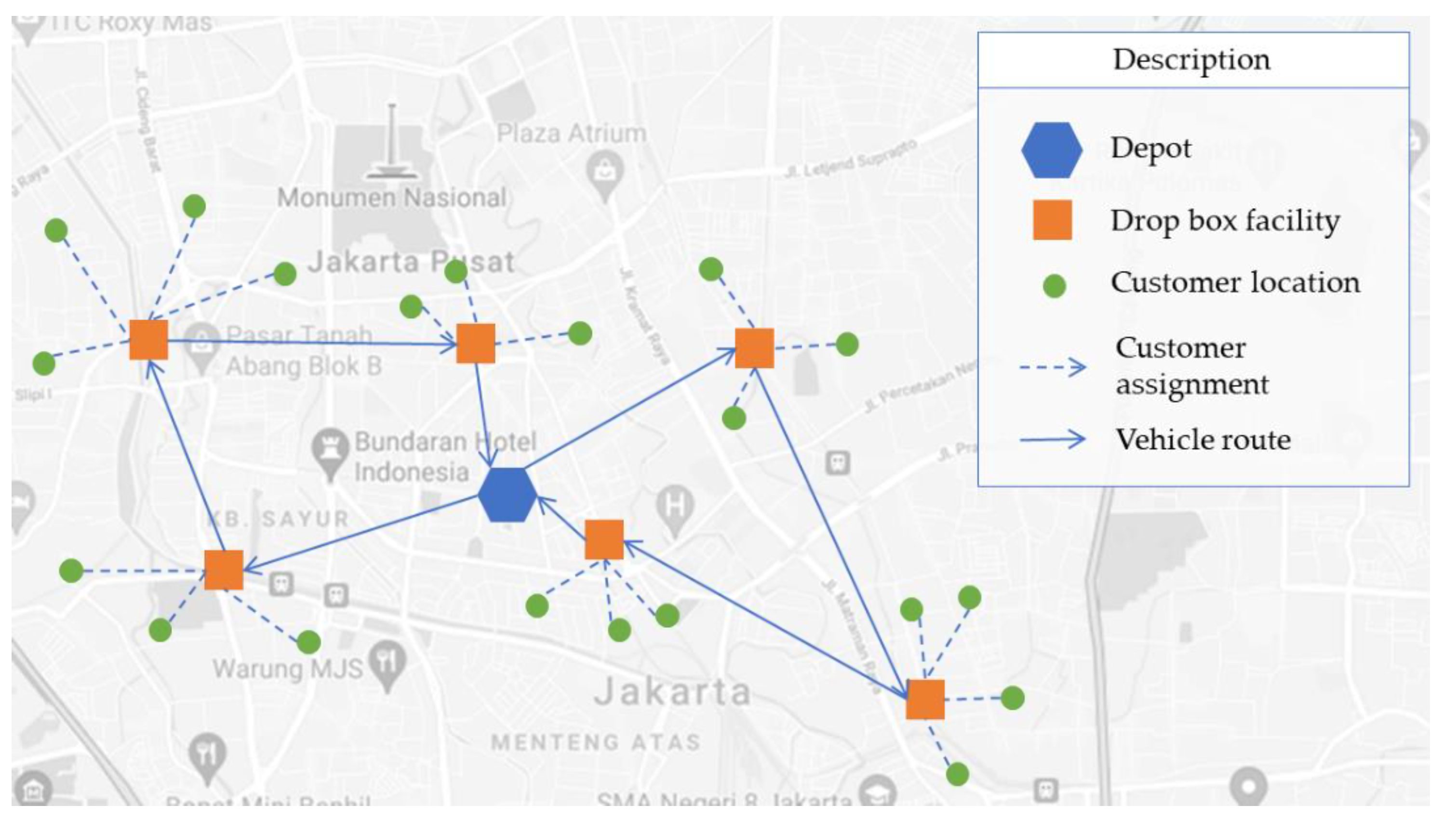
3.2. Solving 2EVRP-DF with Simulated Annealing
3.2.1. SA Parameters
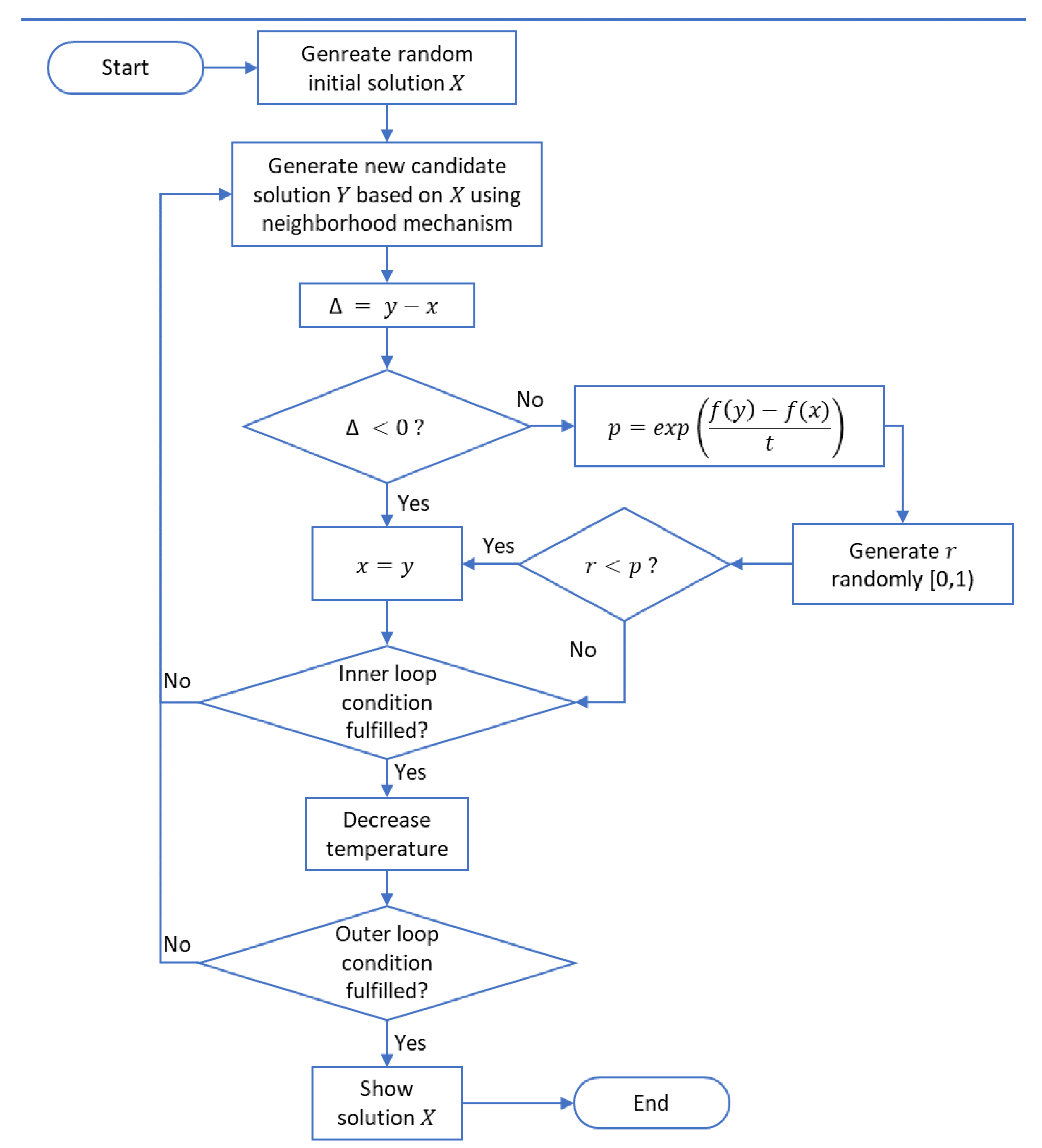
3.2.2. SA Procedure
3.2.3. SA Neighborhood
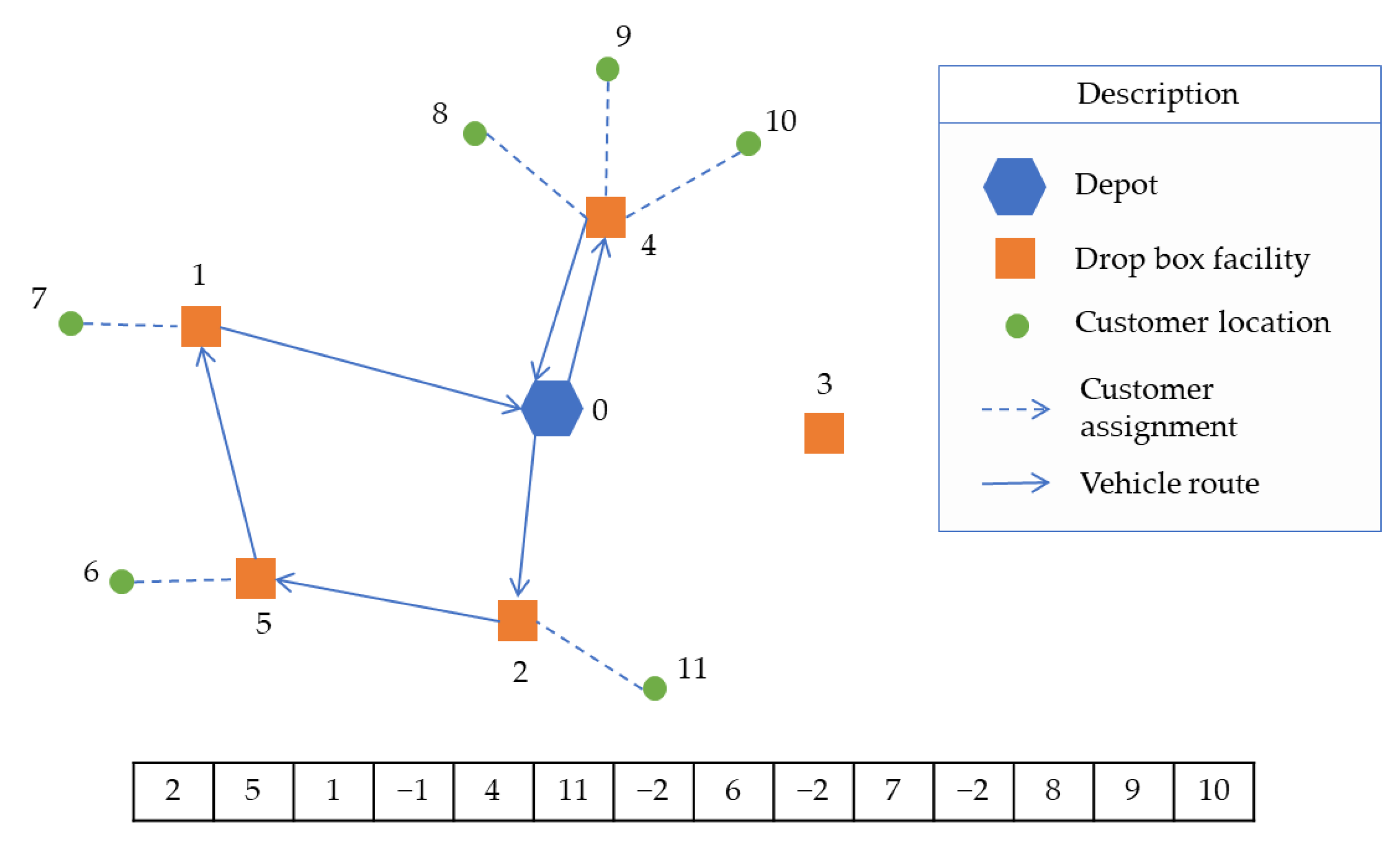
3.2.4. SA Solution Representation
4. Results & Discussion
4.1. Test Instances
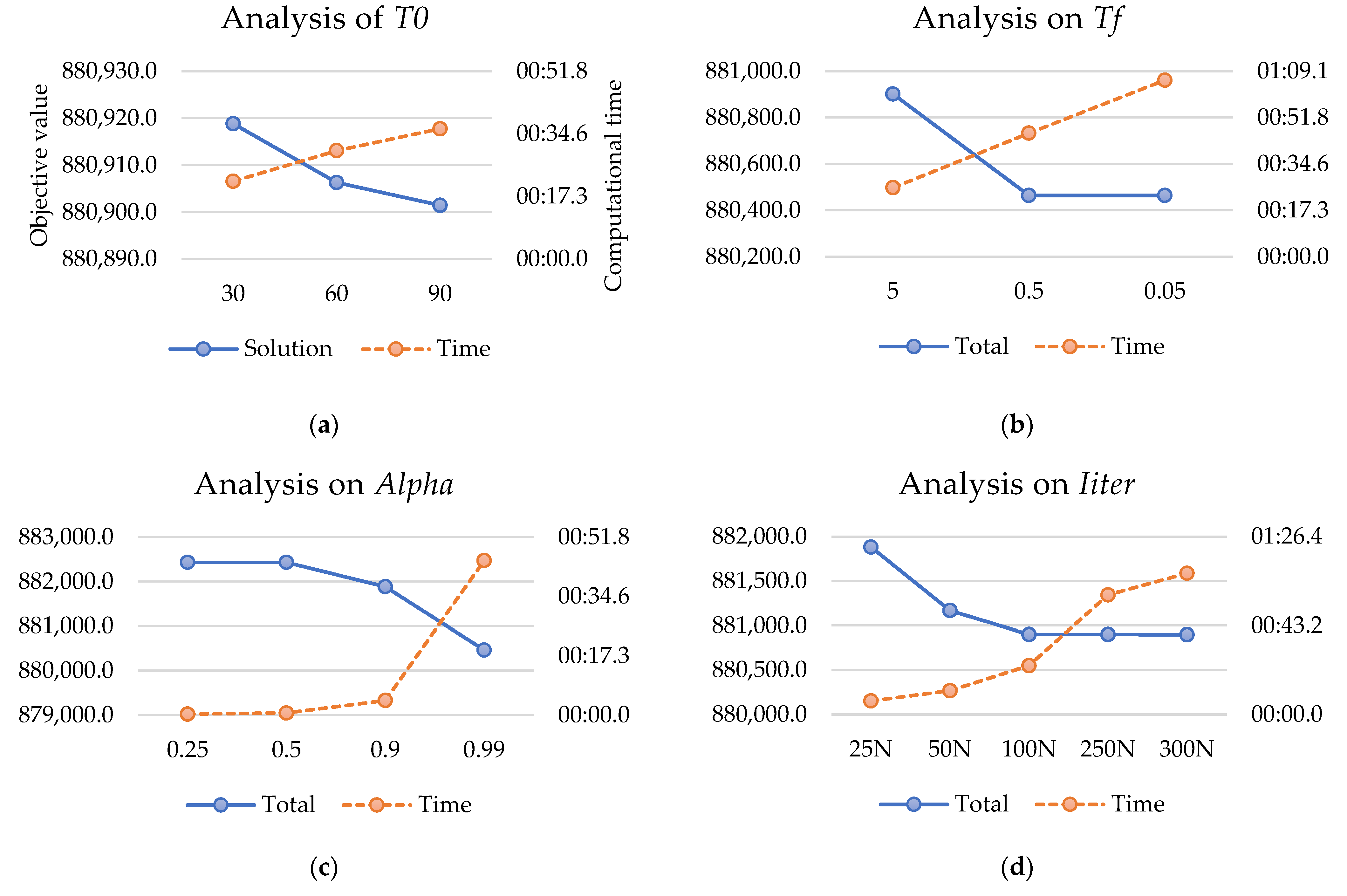
4.2. Parameter Setting
- Initial Temp. (T0): 30, 60, 90
- Final Temp. (Tf): 5, 0.5, 0.05
- Alpha: 0.25, 0.5, 0.9, 0.99
- Iiter: 25N, 50N, 100N, 250N, 300N (N = number of customers)
4.3. Computational Results
5. Conclusions
Author Contributions
Funding
Data Availability Statement
Acknowledgments
Conflicts of Interest
References
- Andianti, R.; Mardiyah, S.; Purba, W.S. Statistik Lingkungan Hidup Indonesia 2020 Environment Statistics of Indonesia 2020; Badan Pusat Statistik/BPS—Statistics Indonesia: Jakarta, Indonesia, 2020. [Google Scholar]
- Badan Pusat Statistik. Proyeksi Penduduk Indonesia 2010–2035; Badan Pusat Statistik/BPS—Statistics Indonesia: Jakarta, Indonesia, 2013. [Google Scholar]
- Mairizal, A.Q.; Sembada, A.Y.; Tse, K.M.; Rhamdhani, M.A. Electronic Waste Generation, Economic Values, Distribution Map, and Possible Recycling System in Indonesia. J. Clean. Prod. 2021, 293, 126096. [Google Scholar] [CrossRef]
- Nurhasanah; Cordova, M.R.; Riani, E. Micro-and Mesoplastics Release from the Indonesian Municipal Solid Waste Landfill Leachate to the Aquatic Environment: Case Study in Galuga Landfill Area, Indonesia. Mar. Pollut. Bull. 2021, 163, 111986. [Google Scholar] [CrossRef] [PubMed]
- Chaabane, A.; Montecinos, J.; Ouhimmou, M.; Khabou, A. Vehicle Routing Problem for Reverse Logistics of End-of-Life Vehicles (ELVs). Waste Manag. 2021, 120, 209–220. [Google Scholar] [CrossRef] [PubMed]
- Geisendorf, S.; Pietrulla, F. The Circular Economy and Circular Economic Concepts—a Literature Analysis and Redefinition. Thunderbird Int. Bus. Rev. 2018, 60, 771–782. [Google Scholar] [CrossRef]
- Lemke, J.; Iwan, S.; Korczak, J. Usability of the Parcel Lockers from the Customer Perspective—The Research in Polish Cities. Transp. Res. Procedia 2016, 16, 272–287. [Google Scholar] [CrossRef] [Green Version]
- Islam, M.A.; Gajpal, Y. Optimization of Conventional and Green Vehicles Composition under Carbon Emission Cap. Sustainability 2021, 13, 6940. [Google Scholar] [CrossRef]
- Fofou, R.F.; Jiang, Z.; Wang, Y. A Review on the Lifecycle Strategies Enhancing Remanufacturing. Appl. Sci. 2021, 11, 5937. [Google Scholar] [CrossRef]
- Redi, A.A.N.; Jewpanya, P.; Kurniawan, A.C.; Persada, S.F.; Nadlifatin, R.; Dewi, O.A.C. A Simulated Annealing Algorithm for Solving Two-Echelon Vehicle Routing Problem with Locker Facilities. Algorithms 2020, 13, 218. [Google Scholar] [CrossRef]
- Deutsch, Y.; Golany, B. A Parcel Locker Network as a Solution to the Logistics Last Mile Problem. Int. J. Prod. Res. 2018, 56, 251–261. [Google Scholar] [CrossRef]
- van Duin, J.H.R.; Wiegmans, B.W.; van Arem, B.; van Amstel, Y. From Home Delivery to Parcel Lockers: A Case Study in Amsterdam. Transp. Res. Procedia 2020, 46, 37–44. [Google Scholar] [CrossRef]
- Perboli, G.; Tadei, R.; Vigo, D. The Two-Echelon Capacitated Vehicle Routing Problem: Models and Math-Based Heuristics. Transp. Sci. 2011, 45, 364–380. [Google Scholar] [CrossRef] [Green Version]
- Cuda, R.; Guastaroba, G.; Speranza, M.G. A Survey on Two-Echelon Routing Problems. Comput. Oper. Res. 2015, 55, 185–199. [Google Scholar] [CrossRef]
- Dellaert, N.; Dashty Saridarq, F.; Van Woensel, T.; Crainic, T.G. Branch-and-Price—Based Algorithms for the Two-Echelon Vehicle Routing Problem with Time Windows. Transp. Sci. 2019, 53, 463–479. [Google Scholar] [CrossRef]
- Baldacci, R.; Mingozzi, A.; Roberti, R.; Calvo, R.W. An Exact Algorithm for the Two-Echelon Capacitated Vehicle Routing Problem. Oper. Res. 2013, 61, 298–314. [Google Scholar] [CrossRef] [Green Version]
- Liu, T.; Luo, Z.; Qin, H.; Lim, A. A Branch-and-Cut Algorithm for the Two-Echelon Capacitated Vehicle Routing Problem with Grouping Constraints. Eur. J. Oper. Res. 2018, 266, 487–497. [Google Scholar] [CrossRef]
- Belgin, O.; Karaoglan, I.; Altiparmak, F. Two-Echelon Vehicle Routing Problem with Simultaneous Pickup and Delivery: Mathematical Model and Heuristic Approach. Comput. Ind. Eng. 2018, 115, 1–16. [Google Scholar] [CrossRef]
- Marques, G.; Sadykov, R.; Deschamps, J.-C.; Dupas, R. An Improved Branch-Cut-and-Price Algorithm for the Two-Echelon Capacitated Vehicle Routing Problem. Comput. Oper. Res. 2020, 114, 104833. [Google Scholar] [CrossRef] [Green Version]
- Elshaer, R.; Awad, H. A Taxonomic Review of Metaheuristic Algorithms for Solving the Vehicle Routing Problem and Its Variants. Comput. Ind. Eng. 2020, 140, 106242. [Google Scholar] [CrossRef]
- Aurachman, R.; Baskara, D.B.; Habibie, J. Vehicle Routing Problem with Simulated Annealing Using Python Programming. IOP Conf. Ser. Mater. Sci. Eng. 2021, 1010, 012010. [Google Scholar] [CrossRef]
- Aydemir, E.; Karagul, K. Solving a Periodic Capacitated Vehicle Routing Problem Using Simulated Annealing Algorithm for a Manufacturing Company. Braz. J. Oper. Prod. Manag. 2020, 17, 1–13. [Google Scholar] [CrossRef] [Green Version]
- Ilhan, I. A Population Based Simulated Annealing Algorithm for Capacitated Vehicle Routing Problem. Turkish J. Electr. Eng. Comput. Sci. 2020, 28, 1217–1235. [Google Scholar] [CrossRef]
- Frans, J.H.; Messah, Y.A.; Issu, N. Kajian Tarif Angkutan Umum Berdasarkan Biaya Operasional Kendaraan (BOK), Ability to Pay (ATP) Dan Willingness to Pay (WTP) Di Kabupaten TTS. J. Tek. Sipil 2016, 5, 185–198. [Google Scholar]
- Ratnawati, D. Indonesian Treasury Review. Indones. Treas. Rev. J. Perbendaharaan, Keuang. Negara Dan Kebijak. Publik 2016, 1, 53–67. [Google Scholar] [CrossRef]
- Kiris, S.B. Carbon Emission Based Optimisation Approach for the Facility Location Problem. Tojsat 2014, 4, 9–20. [Google Scholar]
- Fontaras, G.; Zacharof, N.G.; Ciuffo, B. Fuel Consumption and CO2 Emissions from Passenger Cars in Europe—Laboratory versus Real-World Emissions I. Prog. Energy Combust. Sci. 2017, 60, 97–131. [Google Scholar] [CrossRef]
- Alsumairat, N.; Alrefaei, M. Solving Hybrid-Vehicle Routing Problem Using Modified Simulated Annealing. Int. J. Electr. Comput. Eng. 2021, 11, 4922–4931. [Google Scholar] [CrossRef]
- Rabbouch, B.; Saâdaoui, F.; Mraihi, R. Empirical-Type Simulated Annealing for Solving the Capacitated Vehicle Routing Problem. J. Exp. Theor. Artif. Intell. 2020, 32, 437–452. [Google Scholar] [CrossRef]
- Bernal, J.; Escobar, J.W.; Linfati, R. A Simulated Annealing-Based Approach for a Real Case Study of Vehicle Routing Problem with a Heterogeneous Fleet and Time Windows. Int. J. Shipp. Transp. Logist. 2021, 13, 185–204. [Google Scholar] [CrossRef]
- Sustaination.id. Data Set Drop Box. Available online: https://sustaination.id/dropbox/ (accessed on 7 June 2021).
- Yu, V.F.; Redi, A.A.N.P.; Hidayat, Y.A.; Wibowo, O.J. A Simulated Annealing Heuristic for the Hybrid Vehicle Routing Problem. Appl. Soft Comput. J. 2017, 53, 119–132. [Google Scholar] [CrossRef]
- Theeraviriya, C.; Pitakaso, R.; Sillapasa, K.; Kaewman, S. Location Decision Making and Transportation Route Planning Considering Fuel Consumption. J. Open Innov. Technol. Mark. Complex. 2019, 5, 27. [Google Scholar] [CrossRef] [Green Version]
- Supattananon, N.; Akararungruangkul, R. Modified Differential Evolution Algorithm for a Transportation Software Application. J. Open Innov. Technol. Mark. Complex. 2019, 5, 84. [Google Scholar] [CrossRef] [Green Version]
- Agudelo Zapata, A.A.; Suarez, E.G.; Villegas Florez, J.A. Application of VRP Techniques to the Allocation of Resources in an Electric Power Distribution System. J. Comput. Sci. 2019, 35, 102–109. [Google Scholar] [CrossRef]
- Fermani, M.; Rossit, D.G. A Simulated Annealing Algorithm for Solving a Routing Problem in the Context of Municipal Solid Waste Collection. Int. Conf. Prod. Res. Am. 2021, 1408, 63–76. [Google Scholar]
- Sakamoto, S.; Kulla, E.; Oda, T.; Ikeda, M.; Barolli, L.; Xhafa, F. A Comparison Study of Simulated Annealing and Genetic Algorithm for Node Placement Problem in Wireless Mesh Networks. J. Mob. Multimed. 2013, 9, 101–110. [Google Scholar]
- Wicaksono, P.A.; Puspitasari, D.; Ariyandanu, S.; Hidayanti, R. Comparison of Simulated Annealing, Nearest Neighbour, and Tabu Search Methods to Solve Vehicle Routing Problems. IOP Conf. Ser. Earth Environ. Sci. 2020, 426, 012138. [Google Scholar] [CrossRef]


| Node Facilities & Customers | Latitude | Longitude | Capacity | Demand |
|---|---|---|---|---|
| 0 | −6.2701 | 106.8376 | - | - |
| 1 | −6.25631 | 106.8126 | 15 | - |
| 2 | −6.25693 | 106.8518 | 15 | - |
| 3 | −6.25465 | 106.8138 | 15 | - |
| 4 | −6.28424 | 106.8118 | 15 | - |
| 5 | −6.25153 | 106.8247 | 15 | - |
| 6 | −6.24495 | 106.8287 | - | 5 |
| 7 | −6.26012 | 106.8155 | - | 5 |
| 8 | −6.2746 | 106.8212 | - | 5 |
| 9 | −6.28718 | 106.8012 | - | 5 |
| 10 | −6.27253 | 106.8207 | - | 5 |
| 11 | −6.24853 | 106.8441 | - | 5 |
| Nodes | 0 | 1 | 2 | 3 | 4 | 5 | 6 | 7 | 8 | 9 | 10 | 11 |
|---|---|---|---|---|---|---|---|---|---|---|---|---|
| 0 | 0 | 3.16 | 2.15 | 3.14 | 3.26 | 2.51 | 2.96 | 2.68 | 1.88 | 4.45 | 1.89 | 2.5 |
| 1 | 3.16 | 0 | 4.33 | 0.23 | 3.11 | 1.43 | 2.18 | 0.53 | 2.24 | 3.66 | 2.01 | 3.58 |
| 2 | 2.15 | 4.33 | 0 | 4.21 | 5.37 | 3.06 | 2.88 | 4.03 | 3.92 | 6.53 | 3.86 | 1.27 |
| 3 | 3.14 | 0.23 | 4.21 | 0 | 3.3 | 1.24 | 1.96 | 0.64 | 2.36 | 3.88 | 2.13 | 3.41 |
| 4 | 3.26 | 3.11 | 5.37 | 3.3 | 0 | 3.91 | 4.75 | 2.71 | 1.49 | 1.22 | 1.63 | 5.34 |
| 5 | 2.51 | 1.43 | 3.06 | 1.24 | 3.91 | 0 | 0.86 | 1.39 | 2.59 | 4.74 | 2.38 | 2.17 |
| 6 | 2.96 | 2.18 | 2.88 | 1.96 | 4.75 | 0.86 | 0 | 2.23 | 3.4 | 5.6 | 3.19 | 1.75 |
| 7 | 2.68 | 0.53 | 4.03 | 0.64 | 2.71 | 1.39 | 2.23 | 0 | 1.73 | 3.4 | 1.49 | 3.41 |
| 8 | 1.88 | 2.24 | 3.92 | 2.36 | 1.49 | 2.59 | 3.4 | 1.73 | 0 | 2.62 | 0.24 | 3.85 |
| 9 | 4.45 | 3.66 | 6.53 | 3.88 | 1.22 | 4.74 | 5.6 | 3.4 | 2.62 | 0 | 2.7 | 6.4 |
| 10 | 1.89 | 2.01 | 3.86 | 2.13 | 1.63 | 2.38 | 3.19 | 1.49 | 0.24 | 2.7 | 0 | 3.72 |
| 11 | 2.5 | 3.58 | 1.27 | 3.41 | 5.34 | 2.17 | 1.75 | 3.41 | 3.85 | 6.4 | 3.72 | 0 |
| Customer (N) | Total Demand (kg) | Drop Box (M) | 2EVRP-DF—GUROBI | 2EVRP-DF—SA | Difference | ||||||||||||
|---|---|---|---|---|---|---|---|---|---|---|---|---|---|---|---|---|---|
| E1 (km) | E2 (km) | Emission E1 (kg CO2) | Emission E2 (kg CO2) | Transport Cost (IDR) | Total Emission Cost (IDR) | Total Cost (IDR) | E1 (km) | E2 (km) | Emission E1 (kg CO2) | Emission E2 (kg CO2) | Transport Cost (IDR) | Total Emission Cost (IDR) | Total Cost (IDR) | ||||
| 5 | 40 | 25 | 3.80 | 5.23 | 9.03 | 1.02 | 27,090 | 82 | 27,172 | 3.80 | 5.23 | 1.02 | 0.64 | 27,090 | 133 | 27,223 | 0 |
| 10 | 73 | 25 | 7.70 | 7.49 | 15.19 | 2.07 | 45,570 | 166 | 45,736 | 7.70 | 7.49 | 2.07 | 0.92 | 45,570 | 240 | 45,810 | 0 |
| 15 | 95 | 25 | 7.88 | 10.22 | 18.10 | 2.12 | 54,300 | 170 | 54,470 | 7.88 | 10.22 | 2.12 | 1.25 | 54,300 | 270 | 54,570 | 0 |
| 20 | 124 | 25 | 10.62 | 13.16 | 23.78 | 2.86 | 71,340 | 229 | 71,569 | 10.62 | 13.16 | 2.86 | 1.61 | 71,340 | 358 | 71,698 | 0 |
| 25 | 143 | 25 | 10.82 | 15.29 | 26.11 | 2.91 | 78,330 | 233 | 78,563 | 10.82 | 15.29 | 2.91 | 1.88 | 78,330 | 383 | 78,713 | 0 |
| 30 | 174 | 6 | 12.80 | 41.04 | 30.28 | 3.44 | 90,840 | 275 | 91,115 | 13.05 | 41.04 | 3.51 | 5.04 | 162,270 | 684 | 162,954 | 0 |
| 30 | 174 | 11 | 13.05 | 31.46 | 54.09 | 3.51 | 162,270 | 281 | 162,551 | 13.42 | 31.46 | 3.61 | 3.86 | 134,640 | 598 | 135,238 | 0 |
| 30 | 174 | 16 | 13.42 | 29.29 | 44.88 | 3.61 | 134,640 | 289 | 134,929 | 13.56 | 29.29 | 3.65 | 3.59 | 128,550 | 580 | 129,130 | 0 |
| 30 | 174 | 21 | 13.56 | 18.27 | 42.85 | 3.65 | 128,550 | 292 | 128,842 | 13.65 | 18.27 | 3.67 | 2.24 | 95,760 | 473 | 96,233 | 0 |
| 30 | 174 | 25 | 13.65 | 17.48 | 31.92 | 3.67 | 95,760 | 294 | 96,054 | 12.80 | 17.48 | 3.44 | 2.14 | 90,840 | 448 | 91,288 | 0 |
| Customer (N) | Total Demand (kg) | Drop Box (M) | 2EVRP-DF—GUROBI | 2EVRP-DF—SA | Common Practice (CP) | Cost Diff. GUROBI—CP (%) | Cost Diff. SA—CP (%) | Cost Diff. GUROBI—SA (%) | Time Diff. GUROBI—SA (s) | ||||||||
|---|---|---|---|---|---|---|---|---|---|---|---|---|---|---|---|---|---|
| Transport Cost (Rp) | Emission Cost (IDR) | Total Cost (IDR) | Solved Time (s) | Transport Cost (Rp) | Emission Cost (IDR) | Total Cost (IDR) | Solved Time (s) | Transport Cost (IDR) | Total Emission Cost (IDR) | Total Cost (IDR) | |||||||
| 70 | 527 | 92 | 618,894 | 2833 | 621,727 | 23,822.00 | 613,822 | 2825 | 616,647 | 135.20 | 1,817,917 | 5948 | 1,823,866 | 65.91 | 66.19 | 0.82 | 23,686.80 |
| 80 | 630 | 92 | 712,940 | 3219 | 716,159 | 27,824.40 | 712,044 | 3209 | 715,253 | 163.00 | 2,240,801 | 7332 | 2,248,133 | 68.14 | 68.18 | 0.13 | 27,661.40 |
| 90 | 704 | 92 | 763,551 | 3391 | 766,942 | 26,585.00 | 762,265 | 3386 | 765,651 | 229.60 | 2,551,443 | 8348 | 2,559,792 | 70.04 | 70.09 | 0.17 | 26,355.40 |
| 100 | 786 | 92 | 814,160 | 3549 | 817,709 | 27,099.00 | 812,360 | 3529 | 815,889 | 246.90 | 2,929,518 | 9585 | 2,939,103 | 72.18 | 72.24 | 0.22 | 26,852.10 |
| 110 | 873 | 92 | 874,412 | 3734 | 878,146 | 24,057.20 | 871,158 | 3727 | 874,885 | 287.70 | 3,242,748 | 10,610 | 3,253,358 | 73.01 | 73.11 | 0.37 | 23,769.50 |
| 120 | 964 | 92 | 951,347 | 4050 | 955,397 | 23,137.00 | 951,347 | 4050 | 955,397 | 314.70 | 3,647,314 | 11,934 | 3,659,248 | 73.89 | 73.89 | - | 22,822.30 |
| 130 | 1035 | 92 | 1,010,491 | 4262 | 1,014,753 | 13,455.20 | 1,008,732 | 4239 | 1,012,971 | 393.90 | 3,951,341 | 12,929 | 3,964,270 | 74.40 | 74.45 | 0.18 | 13,061.30 |
| 140 | 1101 | 92 | 1,095,068 | 4568 | 1,099,636 | 18,812.40 | 1,078,093 | 4502 | 1,082,595 | 427.30 | 4,344,548 | 14,215 | 4,358,763 | 74.77 | 75.16 | 1.55 | 18,385.10 |
| 150 | 1194 | 92 | 1,159,221 | 4812 | 1,164,033 | 25,892.00 | 1,145,798 | 4776 | 1,150,574 | 485.90 | 4,673,080 | 15,290 | 4,688,371 | 75.17 | 75.46 | 1.16 | 25,406.10 |
| Average | 888,898 | 3824 | 892,722 | 23,409.36 | 883,958 | 3805 | 887,763 | 298.24 | 3,266,523 | 10,688 | 3,277,212 | 71.95 | 72.09 | 0.51 | 23,111.11 | ||
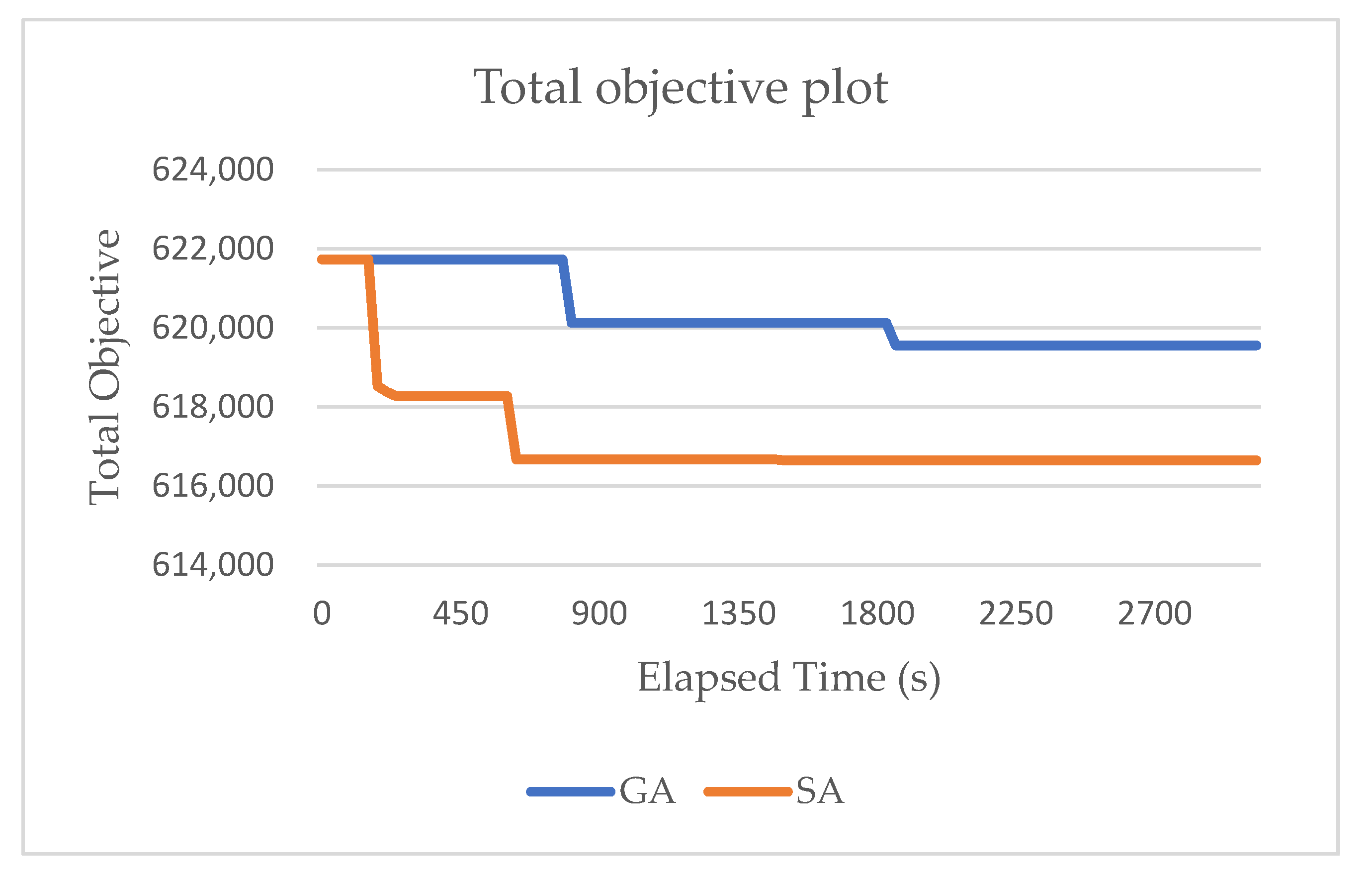
| Customer (N) | Total Demand (kg) | Drop Box (M) | 2EVRP-DF—SA | 2EVRP-DF—GA | Difference | ||||||||||||
|---|---|---|---|---|---|---|---|---|---|---|---|---|---|---|---|---|---|
| E1 (km) | E2 (km) | Emission E1 (kg CO2) | Emission E2 (kg CO2) | Transport Cost (IDR) | Total Emission Cost (IDR) | Total Cost (IDR) | E1 (km) | E2 (km) | Emission E1 (kg CO2) | Emission E2 (kg CO2) | Transport Cost (IDR) | Total Emission Cost (IDR) | Total Cost (IDR) | ||||
| 70 | 527 | 92 | 69.78 | 134.82 | 18.78 | 16.54 | 613,822 | 1502 | 616,647 | 69.06 | 136.52 | 18.58 | 16.75 | 616,729 | 2827 | 619,556 | 0.47 |
| 80 | 630 | 92 | 75.13 | 162.22 | 20.22 | 19.90 | 712,044 | 1617 | 715,253 | 75.74 | 161.91 | 20.38 | 19.87 | 712,940 | 3220 | 716,159 | 0.13 |
| 90 | 704 | 92 | 76.20 | 177.89 | 20.50 | 21.83 | 762,265 | 1640 | 765,651 | 76.27 | 177.86 | 20.52 | 21.82 | 762,393 | 3388 | 765,781 | 0.02 |
| 100 | 786 | 92 | 74.38 | 196.41 | 20.01 | 24.10 | 812,360 | 1601 | 815,889 | 75.52 | 195.87 | 20.32 | 24.03 | 814,159 | 3548 | 817,708 | 0.22 |
| 110 | 873 | 92 | 74.88 | 215.51 | 20.15 | 26.44 | 871,158 | 1612 | 874,885 | 74.56 | 216.52 | 20.06 | 26.57 | 873,254 | 3731 | 876,985 | 0.24 |
| 120 | 964 | 92 | 80.02 | 237.09 | 21.53 | 29.09 | 951,347 | 1723 | 955,397 | 80.02 | 237.09 | 21.53 | 29.09 | 951,346 | 4050 | 955,396 | 0.00 |
| 130 | 1035 | 92 | 80.15 | 256.10 | 21.57 | 31.42 | 1,008,732 | 1725 | 1,012,971 | 80.22 | 256.48 | 21.59 | 31.47 | 1,010,112 | 4245 | 1,014,357 | 0.14 |
| 140 | 1101 | 92 | 83.25 | 276.11 | 22.40 | 33.88 | 1,078,093 | 1792 | 1,082,595 | 84.14 | 276.13 | 22.64 | 33.88 | 1,080,807 | 4522 | 1,085,329 | 0.25 |
| 150 | 1194 | 92 | 87.68 | 294.25 | 23.60 | 36.10 | 1,145,798 | 1888 | 1,150,574 | 87.17 | 296.43 | 23.46 | 36.37 | 1,150,814 | 4786 | 1,155,601 | 0.43 |
| Average | 77.94 | 216.71 | 20.97 | 26.59 | 883,957.67 | 3805.02 | 887,762.69 | 78.08 | 217.20 | 21.01 | 26.65 | 885,839.39 | 3812.90 | 889,652.29 | 0.21 | ||
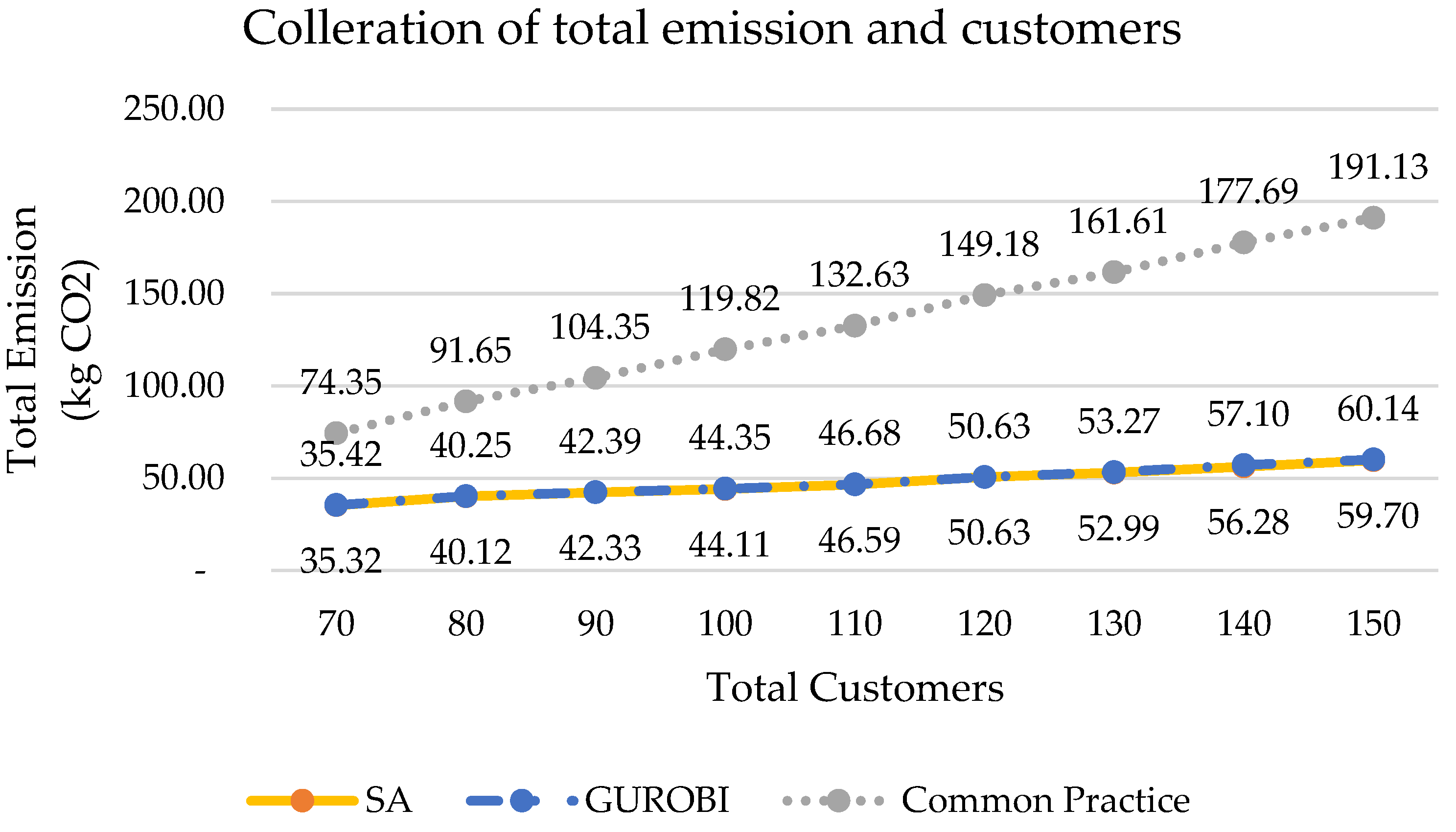
| Customer (N) | Total Demand (kg) | Drop Box (M) | 2EVRP-DF—GUROBI | 2EVRP-DF—SA | Common Practice (CP) | ||||||||||||
|---|---|---|---|---|---|---|---|---|---|---|---|---|---|---|---|---|---|
| E1 (km) | E2 (km) | Emmision E1 (kg CO2) | Emmision E2 (kg CO2) | Total Emission (kg CO2) | Emission Cost (IDR) | E1 (km) | E2 (km) | Emmision E1 (kg CO2) | Emmision E2 (kg CO2) | Total Emission (kg CO2) | Emission Cost (IDR) | Transport Cost (IDR) | Total Emission Cost (IDR) | Total Cost (IDR) | |||
| 70 | 527 | 92 | 69.03 | 137.27 | 18.58 | 16.84 | 35.42 | 2833 | 69.78 | 134.82 | 18.78 | 16.54 | 35.32 | 2825 | 605.97 | 74.35 | 5948 |
| 80 | 630 | 92 | 75.74 | 161.91 | 20.38 | 19.87 | 40.25 | 3219 | 75.13 | 162.22 | 20.22 | 19.90 | 40.12 | 3209 | 746.93 | 91.65 | 7332 |
| 90 | 704 | 92 | 76.24 | 178.28 | 20.52 | 21.87 | 42.39 | 3391 | 76.20 | 177.89 | 20.50 | 21.83 | 42.33 | 3386 | 850.48 | 104.35 | 8348 |
| 100 | 786 | 92 | 75.52 | 195.87 | 20.32 | 24.03 | 44.35 | 3549 | 74.38 | 196.41 | 20.01 | 24.10 | 44.11 | 3529 | 976.51 | 119.82 | 9585 |
| 110 | 873 | 92 | 74.53 | 216.94 | 20.06 | 26.62 | 46.68 | 3734 | 74.88 | 215.51 | 20.15 | 26.44 | 46.59 | 3727 | 1080.92 | 132.63 | 10,610 |
| 120 | 964 | 92 | 80.02 | 237.09 | 21.53 | 29.09 | 50.63 | 4050 | 80.02 | 237.09 | 21.53 | 29.09 | 50.63 | 4050 | 1215.77 | 149.18 | 11,934 |
| 130 | 1035 | 92 | 81.56 | 255.27 | 21.95 | 31.32 | 53.27 | 4262 | 80.15 | 256.10 | 21.57 | 31.42 | 52.99 | 4239 | 1317.11 | 161.61 | 12,929 |
| 140 | 1101 | 92 | 84.09 | 280.93 | 22.63 | 34.47 | 57.10 | 4568 | 83.25 | 276.11 | 22.40 | 33.88 | 56.28 | 4502 | 1448.18 | 177.69 | 14,215 |
| 150 | 1194 | 92 | 86.95 | 299.46 | 23.40 | 36.74 | 60.14 | 4812 | 87.68 | 294.25 | 23.60 | 36.10 | 59.70 | 4776 | 1557.69 | 191.13 | 15,290 |
| Average | 78.19 | 218.11 | 21.04 | 26.76 | 47.80 | 3824 | 77.94 | 216.71 | 20.97 | 26.59 | 47.56 | 3805 | 1088.84 | 133.60 | 10,688 | ||
Publisher’s Note: MDPI stays neutral with regard to jurisdictional claims in published maps and institutional affiliations. |
© 2021 by the authors. Licensee MDPI, Basel, Switzerland. This article is an open access article distributed under the terms and conditions of the Creative Commons Attribution (CC BY) license (https://creativecommons.org/licenses/by/4.0/).
Share and Cite
Reinaldi, M.; Redi, A.A.N.P.; Prakoso, D.F.; Widodo, A.W.; Wibisono, M.R.; Supranartha, A.; Liperda, R.I.; Nadlifatin, R.; Prasetyo, Y.T.; Sakti, S. Solving the Two Echelon Vehicle Routing Problem Using Simulated Annealing Algorithm Considering Drop Box Facilities and Emission Cost: A Case Study of Reverse Logistics Application in Indonesia. Algorithms 2021, 14, 259. https://0-doi-org.brum.beds.ac.uk/10.3390/a14090259
Reinaldi M, Redi AANP, Prakoso DF, Widodo AW, Wibisono MR, Supranartha A, Liperda RI, Nadlifatin R, Prasetyo YT, Sakti S. Solving the Two Echelon Vehicle Routing Problem Using Simulated Annealing Algorithm Considering Drop Box Facilities and Emission Cost: A Case Study of Reverse Logistics Application in Indonesia. Algorithms. 2021; 14(9):259. https://0-doi-org.brum.beds.ac.uk/10.3390/a14090259
Chicago/Turabian StyleReinaldi, Marco, Anak Agung Ngurah Perwira Redi, Dio Fawwaz Prakoso, Arrie Wicaksono Widodo, Mochammad Rizal Wibisono, Agus Supranartha, Rahmad Inca Liperda, Reny Nadlifatin, Yogi Tri Prasetyo, and Sekar Sakti. 2021. "Solving the Two Echelon Vehicle Routing Problem Using Simulated Annealing Algorithm Considering Drop Box Facilities and Emission Cost: A Case Study of Reverse Logistics Application in Indonesia" Algorithms 14, no. 9: 259. https://0-doi-org.brum.beds.ac.uk/10.3390/a14090259