
On Information Granulation via Data Clustering for Granular Computing-Based Pattern Recognition: A Graph Embedding Case Study


Abstract
:1. Introduction
andAmong the basic concepts which underlie human cognition there are three that stand out in importance. The three are: granulation, organization and causation.L.A. Zadeh [3]
Informally, granulation of an object A results in a collection of granules of A, with a granule being a clump of objects (or points) which are drawn together by indistinguishability, similarity, proximity or functionality. In this sense, the granules of a human body are the head, neck, arms, chest, etc. In turn, the granules of a head are the forehead, cheeks, nose, ears, eyes, hair, etc. In general, granulation is hierarchical in nature. A familiar example is granulation of time into years, years in months, months into days and so on.L.A. Zadeh [3]
Language, which is central to most human cognitive activities, is based on granularization. In addition human facilities for distinctions are limited. Being limited, at the very least by language and perhaps additionally by their ability to perceive, human beings have been developed a granular view of the world. Thus, we see that the objects with which humankind perceives, measures, conceptualizes and reasons are granular.R.R. Yager and D. Filev [4]
- Be a truthful representation of the real world;
- Be consistent with human thinking and problem solving;
- Allow a simplification of the problem;
- Provide economic and low-cost solutions.
- Agglomerative clustering algorithms, which work in a bottom-to-top fashion by starting with each data point forming its own cluster and then merging clusters until all data points belong to the same cluster;
- Divisive clustering algorithms, which work in a top-to-bottom fashion by starting with a single cluster embracing the entire dataset and then iteratively splitting the clusters until each data point forms its own cluster.
2. High-Level Framework Description
- Extractor, which is in charge of extracting, from the training set, a suitable set of candidate information granules;
- Granulator, which is in charge of building an alphabet of symbols starting from the candidate information granules provided by the Extractor block;
- Embedder, which is in charge of mapping a graph dataset towards the Euclidean space;
- Classifier, which is in charge of training and testing a suitable classification system in the Euclidean space spanned by the Embedder block.
2.1. Extractor and Granulator
- The union of the three sets yields the original set: ;
- The intersection of any two distinct sets is empty: .
- Q, namely, the maximum number of allowed clusters;
- , namely, the maximum radius for including a pattern into one of the already-discovered clusters;
- A dissimilarity measure between any two patterns.
2.2. Embedder
- The input graph is decomposed into its constituent parts, yielding a decomposition . For the sake of consistency with the Extractor and Granulator modules, in case of path-based subgraphs, the decomposition follows a Breadth First Search strategy, whereas in case of cliques-based granulation, the decomposition follows the maximal clique decomposition.
- For the ith symbol in :
- (a)
- The pairwise dissimilarities between and all subgraphs in are evaluated;
- (b)
- All dissimilarities below a threshold are retained and considered as a ‘hit’;
- (c)
- The ith entry in is filled with the number of occurrences (i.e., the number of ‘hits’);
- Repeat step 2 for .
2.3. Classifier
3. Information Granulation Strategies
3.1. Random Walk
- W, the user-defined number of subgraphs in , i.e., ;
- o, the user-defined maximum number of nodes for subgraphs in .
- Start with ;
- Let be the number of subgraphs to be extracted for each of the candidate subgraph orders;
- For :
- (a)
- Let be a temporary bucket containing only subgraphs of order l;
- (b)
- Until equals :
- i.
- Extract uniformly at random a graph from the training set;
- ii.
- Extract uniformly at random a node v from ;
- iii.
- Start a simple random walk of length l from node v;
- iv.
- The subgraph emerged from the random walk is added to ;
- (c)
- ;
3.2. Clique
- Start with ;
- For each graph from the training set:
- (a)
- (b)
- ;
- Let be a set of W subgraphs selected uniformly at random from ;
- .
3.3. Stratified Clique
- The information about the ground-truth labels (freely available in classification problems) is not exploited in the extraction and granulation stages;
- A uniformly at random selection can bias the contents of , especially in case of unbalanced datasets; indeed, training graphs pertaining to the majority class have a higher change of being selected.
- For each ground-truth class :
- (a)
- Let be the subset of the training set containing only patterns belonging to class i;
- (b)
- Calculate the (relative) frequency of the ith class as , where the operator rounds x to the nearest integer;
- (c)
- Evaluate , namely the size of ;
- (d)
- Set ;
- (e)
- For each graph :
- i.
- Evaluate as the maximal clique decomposition of ;
- ii.
- Update .
- (f)
- If , then replace with a uniform random selection of of its own subgraphs.
- Start with ;
- For each ground-truth class :
- (a)
- Consider the sub-bucket containing subgraphs drawn from ;
- (b)
- Run the Granulator (see Section 3.1) on , yielding ;
- (c)
- .
3.4. Stratified Random Walk
- For each ground-truth class :
- (a)
- Let be the subset of the training set containing only patterns belonging to class i;
- (b)
- Calculate the (relative) frequency of the ith class as ;
- (c)
- Evaluate , namely the size of ;
- (d)
- Evaluate , namely the number of subgraphs to be extracted for each of the candidate subgraphs order, yet considering only graphs belonging to class i;
- (e)
- Set ;
- (f)
- For :
- i.
- Set , namely a temporary bucket that will hold subgraphs of order l extracted from graphs of class i;
- ii.
- Until is equal to :
- A.
- Extract uniformly at random a graph from ;
- B.
- Extract uniformly at random a node v from ;
- C.
- Start a simple random walk of length l from node v;
- D.
- The subgraph emerged from the random walk is added to ;
- iii.
4. Model Synthesis and Testing
- The clustering algorithm parameters for the Granulator block;
- The weights for the nBMF dissimilarity measure (used in both Granulator and Embedder).
- Six real-valued weights that account for the importance of each atomic transformation (insertion, deletion and substitution) on nodes and edges: , , , , , ;
- A set of parameters, if needed, in order to drive the dissimilarity measure between edges;
- A set of parameters, if needed, in order to drive the dissimilarity measure between nodes.
- Projects and on the subset of columns spanned by the indices , say and ;
- Trains the classifier on and validates its performance on .
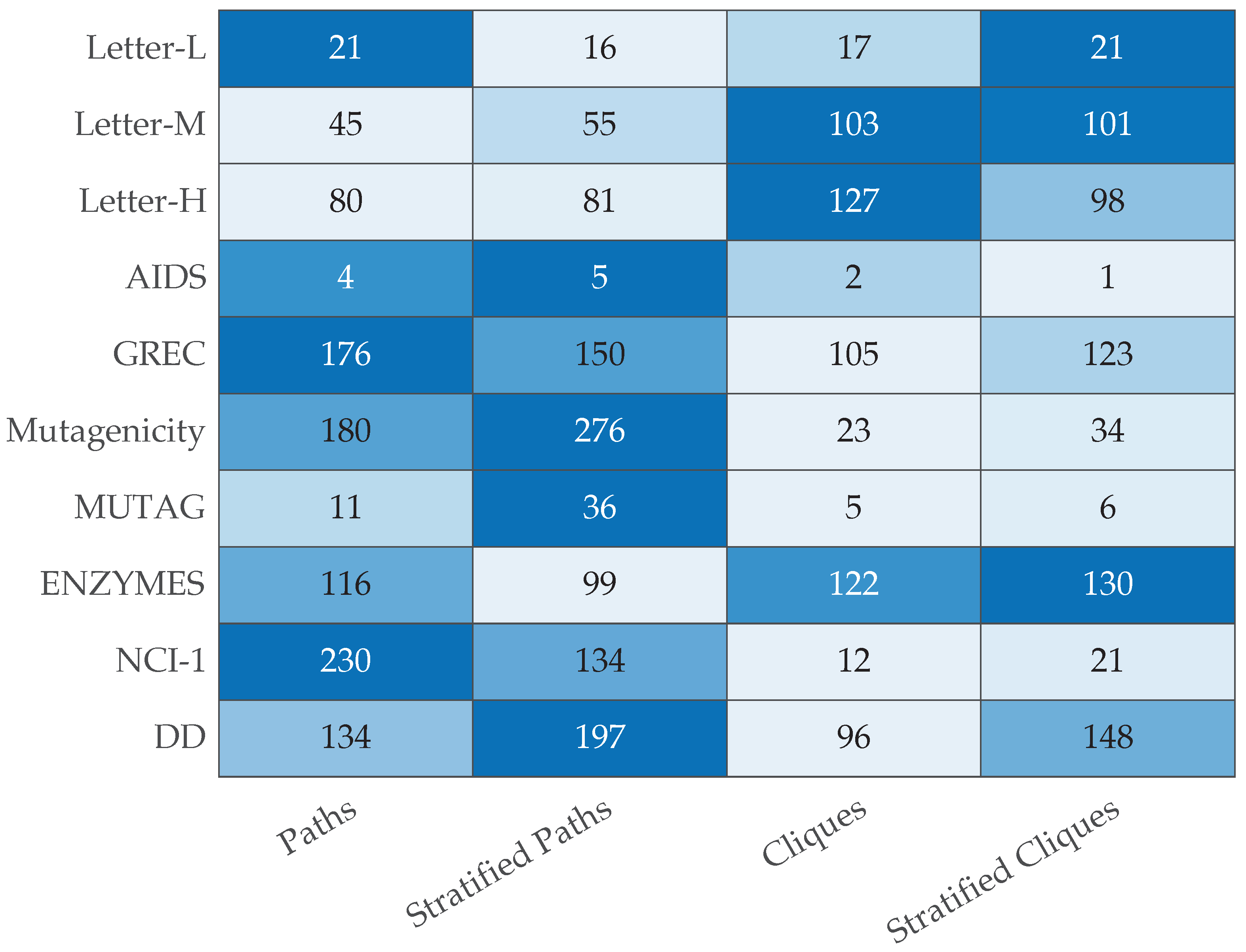
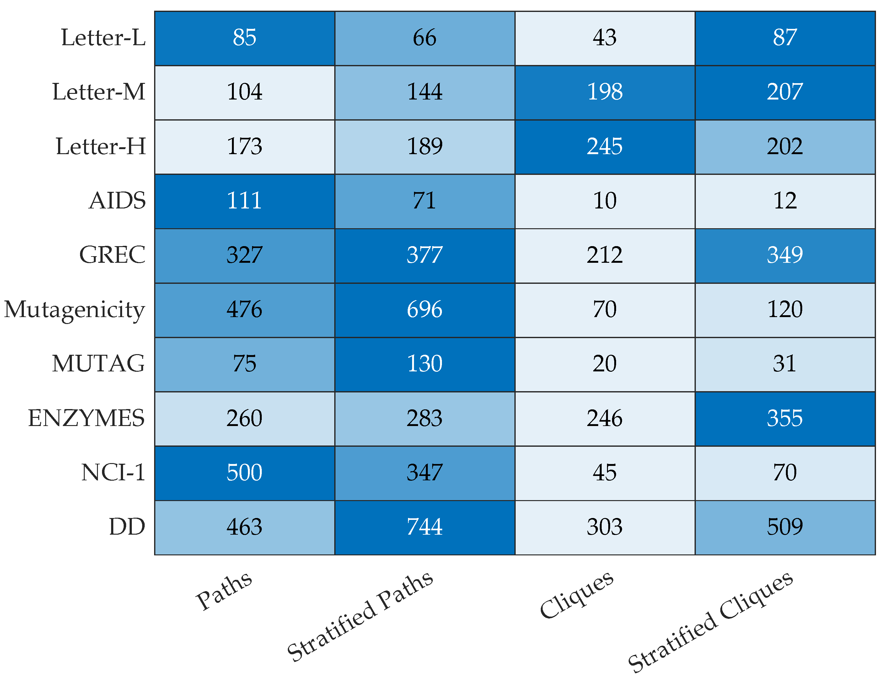
5. Tests and Results
5.1. Datasets Description
- AIDS:
- The AIDS dataset consists of 2000 graphs representing molecules showing activity or not against HIV (two classes). Molecules are converted into graphs in a straightforward manner by representing atoms as nodes and the covalent bonds as edges. Nodes are labeled by a three-element tuple that collects the 2D coordinates of the atom, the chemical symbol (categorical) and its charge (integer). Although edges are originally labeled with the valence of the linkage, such a value has been discarded since it is not useful for the classification task.
- Letter-L:
- The Letter-L dataset involves graphs that represent distorted letter drawings with a low level of distortion. The recognition task involves the 15 capital letters of the Roman alphabet that can be represented by straight lines only. Each handwritten letter is transformed into a graph by representing lines as edges and endpoints of lines as nodes. Each node is labeled by a two-dimensional real-valued vector giving its position within a reference coordinate system. Conversely, edges are unlabeled.
- Letter-M:
- Same as Letter-L, but with medium level of distortion in handwritten digits.
- Letter-H:
- Same as Letter-L, but with high level of distortion in handwritten digits.
- GREC:
- The GREC dataset consists of symbols from electronic and architectural drawings and, after suitable pre-processing, graphs are extracted from such images. Ending points, corners, intersections and circles are represented by nodes and labeled with a two-dimensional attribute giving their position. The nodes are connected by undirected edges, which are labeled as ”line” or ”arc”. An additional attribute specifies the ”angle” with respect to the horizontal direction or the diameter in case of arcs.
- Mutagenicity:
- The Mutagenicity dataset consists of 4337 graphs corresponding to chemical compounds divided into two classes, depending on their respective mutagenic propensity for being a marketable drug or not. Both nodes and edges are equipped with categorical labels: node labels identify the atom type and edge labels identify the valence of the linkage.
- MUTAG:
- The MUTAG dataset consists of 188 graphs corresponding to chemical compounds divided into two classes according to their respective mutagenic effect on a bacterium. Both nodes and edges are equipped with categorical labels: node labels identify the atom type and edge labels identify the bond type (single, double, triple or aromatic).
- DD:
- The DD dataset (also known as D&D) contains 1178 protein structures. Each protein is represented by a graph, in which the nodes are amino-acids and two nodes are connected by an edge if they are less than 6Å apart. Nodes encode a categorical label (i.e., the amino-acid type), whereas edges are unlabeled. The prediction task is to classify the protein structures into enzymes and non-enzymes.
- NCI1:
- Each graph is used as representation of a chemical compound: each vertex stands for an atom of the molecule, and edges between vertices represent bonds between atoms. This dataset is relative to anti-cancer screens, where the chemicals are assessed as positive or negative to cell lung cancer. Each vertex has a categorical label representing the corresponding atom type, whereas edges are unlabeled.
- ENZYMES:
- Each graph represents a simplified protein tertiary structure, where nodes correspond to secondary structure elements and edges connect nodes if those are neighbors along the primary structure (i.e., the amino-acid sequence) with the constraint that every node is connected to its three nearest spatial neighbors. Nodes contain a categorical label stating the type of secondary structure (-helix, -sheet or turn) and a real-valued vector containing 18 physical and chemical measurements. Conversely, edges are unlabeled. The prediction task is used to classify the protein structures into one of the six Enzyme Commission classes [51].
- The dissimilarity between nodes reads as the plain discrete distance between labels;
- The dissimilarity between edges reads as a constant value.
- The dissimilarity between nodes reads as the (normalized) Euclidean distance between their respective 18-length attribute vectors if and only if the two nodes refer to the same secondary structure (i.e., both are -helices, -sheets or turns); otherwise, their dissimilarity is 1;
- The dissimilarity between edges (that are unlabeled) reads as a constant value.
5.2. Algorithmic Setup
- in the fitness function of the first genetic optimization (cf. Equation (8));
- in the fitness function of the second genetic optimization (cf. Equation (12));
- Maximum number of 20 generations for both genetic optimizations;
- A total of 20 and 100 individuals in the population for the first and second genetic optimization, respectively;
- Maximum walk length ;
- Candidate values are ;
- , where for non-stratified Granulators and for stratified Granulators [41];
- The user-defined bucket size W has been chosen according to a given percentage of the maximum number of paths or cliques that can be drawn from the training graphs. The percentages are chosen according to the following rule: the larger the dataset, the higher the subsampling rate. For the sake of shorthand, we omit any sensitivity analysis on the behavior of the Granulators as a function of W. In this regard, we refer the interested reader to our previous works [41,46,66] The values for W for both clique-based and path-based Granulators are summarized in Table 2.
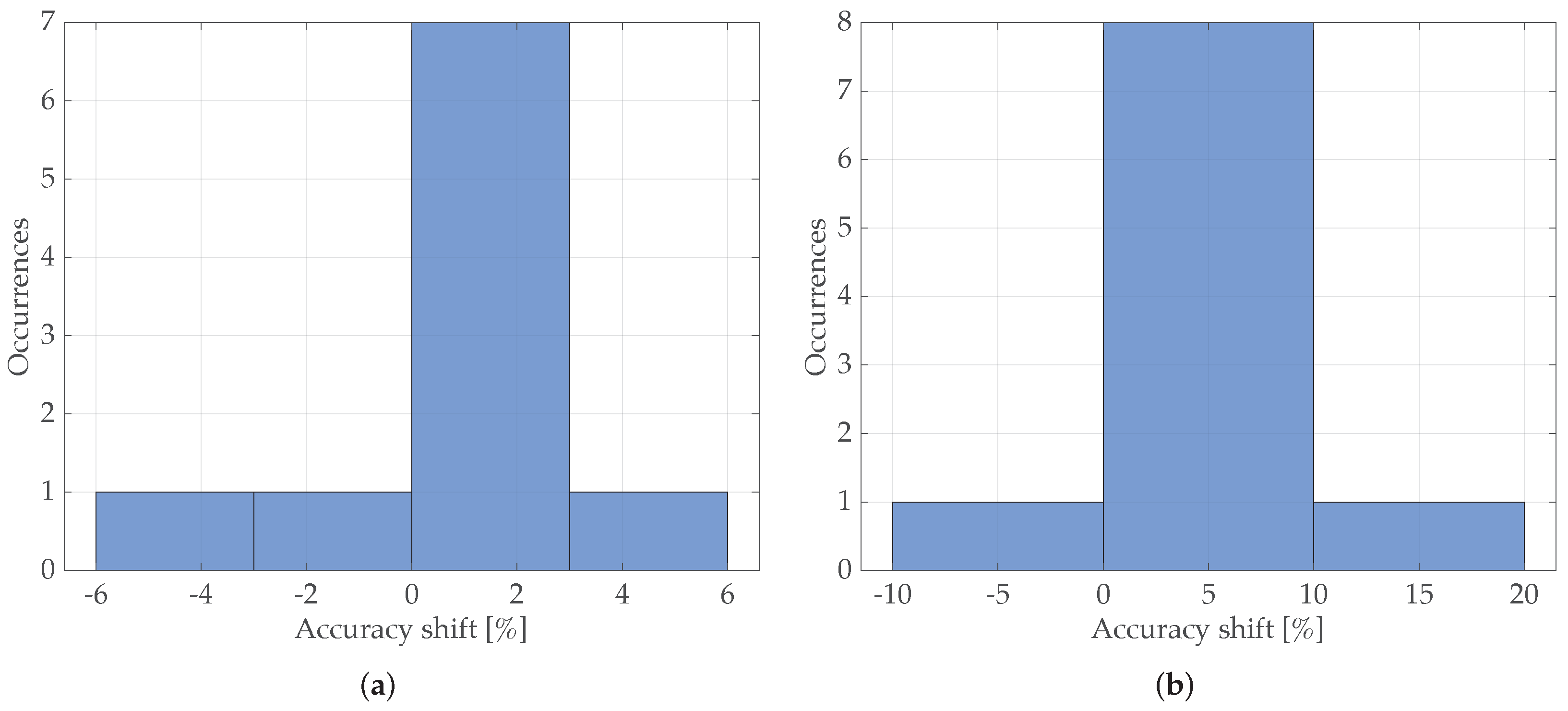
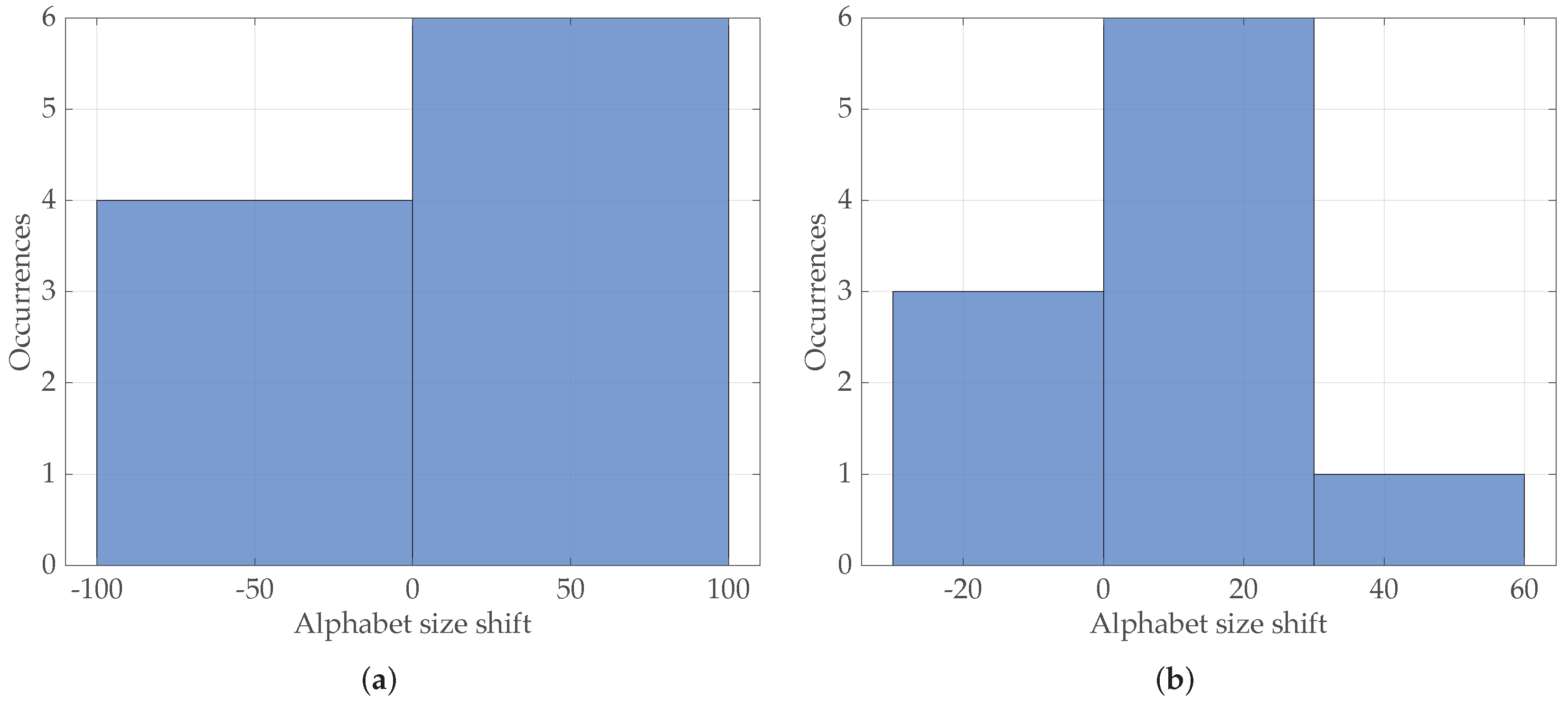
5.3. Computational Results
6. Conclusions
Author Contributions
Funding
Institutional Review Board Statement
Informed Consent Statement
Data Availability Statement
Conflicts of Interest
Abbreviations
| BSAS | Basic Sequential Algorithmic Scheme |
| GRALG | GRanular computing Approach for labeled Graphs |
| GED | Graph Edit Distance |
| K-NN | K-Nearest Neighbors |
| nBMF | node Best Match First |
References
- Bargiela, A.; Pedrycz, W. Granular Computing: An Introduction; Kluwer Academic Publishers: Boston, MA, USA, 2003. [Google Scholar]
- Pedrycz, W.; Skowron, A.; Kreinovich, V. Handbook of Granular Computing; John Wiley & Sons: Hoboken, NJ, USA, 2008. [Google Scholar]
- Zadeh, L.A. Toward a theory of fuzzy information granulation and its centrality in human reasoning and fuzzy logic. Fuzzy Sets Syst. 1997, 90, 111–127. [Google Scholar] [CrossRef]
- Yager, R.; Filev, D. Operations for granular computing: Mixing words and numbers. In Proceedings of the 1998 IEEE International Conference on Fuzzy Systems Proceedings, IEEE World Congress on Computational Intelligence (Cat. No.98CH36228), Anchorage, AK, USA, 4–9 May 1998; Volume 1, pp. 123–128. [Google Scholar] [CrossRef]
- Zadeh, L. Fuzzy logic = computing with words. IEEE Trans. Fuzzy Syst. 1996, 4, 103–111. [Google Scholar] [CrossRef] [Green Version]
- Yao, Y. Perspectives of granular computing. In Proceedings of the 2005 IEEE International Conference on Granular Computing, Beijing, China, 25–27 July 2005; Volume 1, pp. 85–90. [Google Scholar]
- Pedrycz, A.; Hirota, K.; Pedrycz, W.; Dong, F. Granular representation and granular computing with fuzzy sets. Fuzzy Sets Syst. 2012, 203, 17–32. [Google Scholar] [CrossRef]
- Dubois, D.; Prade, H. Bridging gaps between several forms of granular computing. Granul. Comput. 2016, 1, 115–126. [Google Scholar] [CrossRef] [Green Version]
- Pawlak, Z. Rough sets. Int. J. Comput. Inf. Sci. 1982, 11, 341–356. [Google Scholar] [CrossRef]
- Zhang, Q.; Zhang, Q.; Wang, G. The Uncertainty of Probabilistic Rough Sets in Multi-Granulation Spaces. Int. J. Approx. Reason. 2016, 77, 38–54. [Google Scholar] [CrossRef]
- Pedrycz, W. Shadowed sets: Representing and processing fuzzy sets. IEEE Trans. Syst. Man Cybern. Part B 1998, 28, 103–109. [Google Scholar] [CrossRef]
- Kreinovich, V. Interval Computation as an Important Part of Granular Computing: An Introduction. In Handbook of Granular Computing; John Wiley & Sons, Ltd.: Hoboken, NJ, USA, 2008; pp. 1–31. [Google Scholar] [CrossRef]
- Pedrycz, W. Proximity-based clustering: A search for structural consistency in data with semantic blocks of features. IEEE Trans. Fuzzy Syst. 2013, 21, 978–982. [Google Scholar] [CrossRef]
- Ding, S.; Du, M.; Zhu, H. Survey on granularity clustering. Cogn. Neurodyn. 2015, 9, 561–572. [Google Scholar] [CrossRef] [Green Version]
- Peters, G.; Weber, R. DCC: A framework for dynamic granular clustering. Granul. Comput. 2016, 1, 1–11. [Google Scholar] [CrossRef] [Green Version]
- Jain, A.K.; Murty, M.N.; Flynn, P.J. Data Clustering: A Review. ACM Comput. Surv. 1999, 31, 264–323. [Google Scholar] [CrossRef]
- Hadamard, J. Sur les problèmes aux dérivés partielles et leur signification physique. Princet. Univ. Bull. 1902, 13, 49–52. [Google Scholar]
- von Luxburg, U.; Williamson, R.C.; Guyon, I. Clustering: Science or Art? In Proceedings of ICML Workshop on Unsupervised and Transfer Learning; Guyon, I., Dror, G., Lemaire, V., Taylor, G., Silver, D., Eds.; PMLR: Bellevue, WA, USA, 2012; Volume 27, pp. 65–79. [Google Scholar]
- Bouveyron, C.; Hammer, B.; Villmann, T. Recent developments in clustering algorithms. In ESANN 2012; ESANN: Bruges, Belgium, 2012; pp. 447–458. [Google Scholar]
- Xu, R.; Wunsch, D. Survey of clustering algorithms. IEEE Trans. Neural Netw. 2005, 16, 645–678. [Google Scholar] [CrossRef] [PubMed] [Green Version]
- MacQueen, J. Some methods for classification and analysis of multivariate observations. In Proceedings of the Fifth Berkeley Symposium on Mathematical Statistics and Probability, Oakland, CA, USA, 21 June–18 July 1967; Volume 1, pp. 281–297. [Google Scholar]
- Kaufman, L.; Rousseeuw, P. Clustering by means of Medoids. In Statistical Data Analysis Based on the L1 Norm and Related Methods; Dodge, Y., Ed.; Elsevier: Amsterdam, The Netherlands, 1987; pp. 405–416. [Google Scholar]
- Huang, Z. Clustering large data sets with mixed numeric and categorical values. In Proceedings of the First Pacific Asia Knowledge Discovery and Data Mining Conference, Singapore, 23–24 February 1997; pp. 21–34. [Google Scholar]
- Bezdek, J.C. Pattern Recognition with Fuzzy Objective Function Algorithms; Kluwer Academic Publishers: Norwell, MA, USA, 1981. [Google Scholar]
- Livi, L.; Del Vescovo, G.; Rizzi, A. Graph Recognition by Seriation and Frequent Substructures Mining. In Proceedings of the ICPRAM 2012—1st International Conference on Pattern Recognition Applications and Methods, Algarve, Portugal, 6–8 February 2012; Volume 1, pp. 186–191. [Google Scholar]
- Rizzi, A.; Del Vescovo, G. Automatic Image Classification by a Granular Computing Approach. In Proceedings of the 2006 16th IEEE Signal Processing Society Workshop on Machine Learning for Signal Processing, Maynooth, Ireland, 6–8 September 2006; pp. 33–38. [Google Scholar] [CrossRef]
- Hastie, T.; Tibshirani, R.; Friedman, J. The Elements of Statistical Learning: Data Mining, Inference, and Prediction, 2nd ed.; Springer: Berlin/Heidelberg, Germany, 2009. [Google Scholar]
- Pedrycz, W. Knowledge-Based Clustering: From Data to Information Granules; John Wiley & Sons: Hoboken, NJ, USA, 2005. [Google Scholar]
- Theodoridis, S.; Koutroumbas, K. Pattern Recognition, 4th ed.; Academic Press: Cambridge, MA, USA, 2008. [Google Scholar]
- Sanfeliu, A.; Fu, K.S. A distance measure between attributed relational graphs for pattern recognition. IEEE Trans. Syst. Man Cybern. 1983, SMC-13, 353–362. [Google Scholar] [CrossRef]
- Gao, X.; Xiao, B.; Tao, D.; Li, X. A survey of graph edit distance. Pattern Anal. Appl. 2010, 13, 113–129. [Google Scholar] [CrossRef]
- Martino, A.; Rizzi, A. An Enhanced Filtering-Based Information Granulation Procedure for Graph Embedding and Classification. IEEE Access 2021, 9, 15426–15440. [Google Scholar] [CrossRef]
- Baldini, L.; Martino, A.; Rizzi, A. Relaxed Dissimilarity-based Symbolic Histogram Variants for Granular Graph Embedding. In Proceedings of the 13th International Joint Conference on Computational Intelligence—NCTA, Singapore, 10–13 November 2021; pp. 221–235. [Google Scholar] [CrossRef]
- Cover, T.; Hart, P. Nearest neighbor pattern classification. IEEE Trans. Inf. Theory 1967, 13, 21–27. [Google Scholar] [CrossRef]
- Lovász, L. Random walks on graphs: A survey. Combinatorics 1993, 2, 1–46. [Google Scholar]
- Göbel, F.; Jagers, A.A. Random walks on graphs. Stoch. Process. Their Appl. 1974, 2, 311–336. [Google Scholar] [CrossRef] [Green Version]
- Pedrycz, W.; Homenda, W. Building the fundamentals of granular computing: A principle of justifiable granularity. Appl. Soft Comput. 2013, 13, 4209–4218. [Google Scholar] [CrossRef]
- Wang, G.; Yang, J.; Xu, J. Granular computing: From granularity optimization to multi-granularity joint problem solving. Granul. Comput. 2017, 2, 105–120. [Google Scholar] [CrossRef]
- Yao, Y.Y. The rise of granular computing. J. Chongqing Univ. Posts Telecommun. 2008, 20, 299–308. [Google Scholar]
- Yao, Y.; Zhao, L. A measurement theory view on the granularity of partitions. Inf. Sci. 2012, 213, 1–13. [Google Scholar] [CrossRef]
- Baldini, L.; Martino, A.; Rizzi, A. Towards a Class-Aware Information Granulation for Graph Embedding and Classification. In Computational Intelligence, Proceedings of the 11th International Joint Conference, IJCCI 2019, Vienna, Austria, 17–19 September 2019, Revised Selected Papers; Merelo, J.J., Garibaldi, J., Linares-Barranco, A., Warwick, K., Madani, K., Eds.; Springer International Publishing: Cham, Switzerland, 2021; pp. 263–290. [Google Scholar] [CrossRef]
- Tichy, N. An Analysis of Clique Formation and Structure in Organizations. Adm. Sci. Q. 1973, 18, 194–208. [Google Scholar] [CrossRef]
- Luce, R.D.; Perry, A.D. A method of matrix analysis of group structure. Psychometrika 1949, 14, 95–116. [Google Scholar] [CrossRef] [PubMed]
- Bron, C.; Kerbosch, J. Algorithm 457: Finding All Cliques of an Undirected Graph. Commun. ACM 1973, 16, 575–577. [Google Scholar] [CrossRef]
- Moon, J.W.; Moser, L. On cliques in graphs. Isr. J. Math. 1965, 3, 23–28. [Google Scholar] [CrossRef]
- Baldini, L.; Martino, A.; Rizzi, A. Exploiting Cliques for Granular Computing-based Graph Classification. In Proceedings of the 2020 International Joint Conference on Neural Networks (IJCNN), Glasgow, UK, 19–24 July 2020; pp. 1–9. [Google Scholar] [CrossRef]
- Storn, R.; Price, K. Differential Evolution—A Simple and Efficient Heuristic for global Optimization over Continuous Spaces. J. Glob. Optim. 1997, 11, 341–359. [Google Scholar] [CrossRef]
- Grandini, M.; Bagli, E.; Visani, G. Metrics for Multi-Class Classification: An Overview. arXiv 2020, arXiv:2008.05756. [Google Scholar]
- Riesen, K.; Bunke, H. IAM Graph Database Repository for Graph Based Pattern Recognition and Machine Learning. In Structural, Syntactic, and Statistical Pattern Recognition; da Vitoria Lobo, N., Kasparis, T., Roli, F., Kwok, J.T., Georgiopoulos, M., Anagnostopoulos, G.C., Loog, M., Eds.; Springer: Berlin/Heidelberg, Germany, 2008; pp. 287–297. [Google Scholar]
- Morris, C.; Kriege, N.M.; Bause, F.; Kersting, K.; Mutzel, P.; Neumann, M. TUDataset: A collection of benchmark datasets for learning with graphs. ICML 2020 Workshop on Graph Representation Learning and Beyond (GRL+ 2020). arXiv 2020, arXiv:2007.08663. [Google Scholar]
- Webb, E.C. Enzyme Nomenclature 1992. Recommendations of the Nomenclature Committee of the International Union of Biochemistry and Molecular Biology on the Nomenclature and Classification of Enzymes, 6th ed.; Academic Press: Cambridge, MA, USA, 1992. [Google Scholar]
- Dosch, P.; Valveny, E. Report on the Second Symbol Recognition Contest. In Graphics Recognition. Ten Years Review and Future Perspectives; Liu, W., Lladós, J., Eds.; Springer Berlin Heidelberg: Berlin/Heidelberg, Germany, 2006; pp. 381–397. [Google Scholar]
- Kazius, J.; McGuire, R.; Bursi, R. Derivation and Validation of Toxicophores for Mutagenicity Prediction. J. Med. Chem. 2005, 48, 312–320. [Google Scholar] [CrossRef] [PubMed]
- Debnath, A.K.; Lopez de Compadre, R.L.; Debnath, G.; Shusterman, A.J.; Hansch, C. Structure-activity relationship of mutagenic aromatic and heteroaromatic nitro compounds. Correlation with molecular orbital energies and hydrophobicity. J. Med. Chem. 1991, 34, 786–797. [Google Scholar] [CrossRef] [PubMed]
- Kriege, N.; Mutzel, P. Subgraph Matching Kernels for Attributed Graphs. In Proceedings of the 29th International Coference on International Conference on Machine Learning, Edinburgh, UK, 27 June–3 July 2012; Omnipress: Madison, WI, USA, 2012; Volume ICML’12, pp. 291–298. [Google Scholar]
- Dobson, P.D.; Doig, A.J. Distinguishing Enzyme Structures from Non-enzymes without Alignments. J. Mol. Biol. 2003, 330, 771–783. [Google Scholar] [CrossRef] [Green Version]
- Shervashidze, N.; Schweitzer, P.; van Leeuwen, E.J.; Mehlhorn, K.; Borgwardt, K.M. Weisfeiler-Lehman Graph Kernels. J. Mach. Learn. Res. 2011, 12, 2539–2561. [Google Scholar]
- Wale, N.; Karypis, G. Comparison of Descriptor Spaces for Chemical Compound Retrieval and Classification. In Proceedings of the Sixth International Conference on Data Mining (ICDM’06), Hong Kong, China, 18–22 December 2006; pp. 678–689. [Google Scholar] [CrossRef] [Green Version]
- Schomburg, I.; Chang, A.; Ebeling, C.; Gremse, M.; Heldt, C.; Huhn, G.; Schomburg, D. BRENDA, the enzyme database: Updates and major new developments. Nucleic Acids Res. 2004, 32, D431–D433. [Google Scholar] [CrossRef] [PubMed] [Green Version]
- Borgwardt, K.M.; Ong, C.S.; Schönauer, S.; Vishwanathan, S.V.N.; Smola, A.J.; Kriegel, H.P. Protein function prediction via graph kernels. Bioinformatics 2005, 21, i47–i56. [Google Scholar] [CrossRef] [Green Version]
- Deza, M.M.; Deza, E. Encyclopedia of Distances, 1st ed.; Springer: Berlin/Heidelberg, Germany, 2009. [Google Scholar]
- Hagberg, A.A.; Schult, D.A.; Swart, P.J. Exploring Network Structure, Dynamics, and Function using NetworkX. In Proceedings of the 7th Python in Science Conference; Varoquaux, G., Vaught, T., Millman, J., Eds.; Los Alamos National Lab.: Pasadena, CA, USA, 2008; pp. 11–15. [Google Scholar]
- Rozemberczki, B.; Kiss, O.; Sarkar, R. Little Ball of Fur: A Python Library for Graph Sampling. In Proceedings of the 29th ACM International Conference on Information and Knowledge Management (CIKM ’20), Online. 19–23 October 2020; pp. 3133–3140. [Google Scholar]
- Pedregosa, F.; Varoquaux, G.; Gramfort, A.; Michel, V.; Thirion, B.; Grisel, O.; Blondel, M.; Prettenhofer, P.; Weiss, R.; Dubourg, V.; et al. Scikit-learn: Machine Learning in Python. J. Mach. Learn. Res. 2011, 12, 2825–2830. [Google Scholar]
- Virtanen, P.; Gommers, R.; Oliphant, T.E.; Haberland, M.; Reddy, T.; Cournapeau, D.; Burovski, E.; Peterson, P.; Weckesser, W.; Bright, J.; et al. SciPy 1.0: Fundamental Algorithms for Scientific Computing in Python. Nat. Methods 2020, 17, 261–272. [Google Scholar] [CrossRef] [Green Version]
- Baldini, L.; Martino, A.; Rizzi, A. Stochastic Information Granules Extraction for Graph Embedding and Classification. In Proceedings of the 11th International Joint Conference on Computational Intelligence, NCTA, (IJCCI 2019), Hendaye, France, 4–6 September 2019; Volume 1, pp. 391–402. [Google Scholar] [CrossRef]
- Riesen, K.; Bunke, H. Approximate graph edit distance computation by means of bipartite graph matching. Image Vis. Comput. 2009, 27, 950–959. [Google Scholar] [CrossRef]
- Conte, D.; Ramel, J.Y.; Sidère, N.; Luqman, M.M.; Gaüzère, B.; Gibert, J.; Brun, L.; Vento, M. A Comparison of Explicit and Implicit Graph Embedding Methods for Pattern Recognition. In Graph-Based Representations in Pattern Recognition; Kropatsch, W.G., Artner, N.M., Haxhimusa, Y., Jiang, X., Eds.; Springer: Berlin/Heidelberg, Germany, 2013; pp. 81–90. [Google Scholar] [CrossRef] [Green Version]
- Da San Martino, G.; Navarin, N.; Sperduti, A. Ordered Decompositional DAG kernels enhancements. Neurocomputing 2016, 192, 92–103. [Google Scholar] [CrossRef] [Green Version]
- Martino, A.; Rizzi, A. (Hyper)graph Kernels over Simplicial Complexes. Entropy 2020, 22, 1155. [Google Scholar] [CrossRef] [PubMed]
- Yanardag, P.; Vishwanathan, S. Deep Graph Kernels. In Proceedings of the 21th ACM SIGKDD International Conference on Knowledge Discovery and Data Mining; Association for Computing Machinery: New York, NY, USA, 2015; Volume KDD ’15, pp. 1365–1374. [Google Scholar] [CrossRef]
- Riesen, K.; Bunke, H. Graph Classification by Means of Lipschitz Embedding. IEEE Trans. Syst. Man, Cybern. Part B Cybern. 2009, 39, 1472–1483. [Google Scholar] [CrossRef] [PubMed]
- Gibert, J.; Valveny, E.; Bunke, H. Dimensionality Reduction for Graph of Words Embedding. In Graph-Based Representations in Pattern Recognition; Jiang, X., Ferrer, M., Torsello, A., Eds.; Springer: Berlin/Heidelberg, Germany, 2011; pp. 22–31. [Google Scholar]
- Martino, A.; Giuliani, A.; Rizzi, A. (Hyper)Graph Embedding and Classification via Simplicial Complexes. Algorithms 2019, 12, 223. [Google Scholar] [CrossRef] [Green Version]
- Ma, Y.; Wang, S.; Aggarwal, C.C.; Tang, J. Graph Convolutional Networks with EigenPooling. In Proceedings of the 25th ACM SIGKDD International Conference on Knowledge Discovery & Data Mining; Association for Computing Machinery: New York, NY, USA, 2019; Volume KDD ’19, pp. 723–731. [Google Scholar] [CrossRef] [Green Version]
- Bacciu, D.; Errica, F.; Micheli, A. Contextual graph markov model: A deep and generative approach to graph processing. In Proceedings of the 35th International Conference on Machine Learning, ICML 2018, Stockholm, Sweden, 10–15 July 2018; Volume 1, pp. 495–504. [Google Scholar]
- Martineau, M.; Raveaux, R.; Conte, D.; Venturini, G. Learning error-correcting graph matching with a multiclass neural network. Pattern Recognit. Lett. 2020, 134, 68–76. [Google Scholar] [CrossRef] [Green Version]
- Kajla, N.I.; Missen, M.M.S.; Luqman, M.M.; Coustaty, M. Graph Neural Networks Using Local Descriptions in Attributed Graphs: An Application to Symbol Recognition and Hand Written Character Recognition. IEEE Access 2021, 9, 99103–99111. [Google Scholar] [CrossRef]
- Riba, P.; Dutta, A.; Lladós, J.; Fornés, A. Graph-Based Deep Learning for Graphics Classification. In Proceedings of the 2017 14th IAPR International Conference on Document Analysis and Recognition (ICDAR), Kyoto, Japan, 13–15 November 2017; Volume 2, pp. 29–30. [Google Scholar] [CrossRef] [Green Version]
- Sidère, N.; Héroux, P.; Ramel, J.Y. Vector Representation of Graphs: Application to the Classification of Symbols and Letters. In Proceedings of the 2009 10th International Conference on Document Analysis and Recognition, Barcelona, Spain, 26–29 July 2009; pp. 681–685. [Google Scholar] [CrossRef] [Green Version]
- Luqman, M.M.; Ramel, J.Y.; Lladós, J.; Brouard, T. Fuzzy multilevel graph embedding. Pattern Recognit. 2013, 46, 551–565. [Google Scholar] [CrossRef]
- Gibert, J.; Valveny, E.; Bunke, H. Graph embedding in vector spaces by node attribute statistics. Pattern Recognit. 2012, 45, 3072–3083. [Google Scholar] [CrossRef]
- Brun, L.; Conte, D.; Foggia, P.; Vento, M. A Graph-Kernel Method for Re-identification. In Image Analysis and Recognition; Kamel, M., Campilho, A., Eds.; Springer: Berlin/Heidelberg, Germany, 2011; pp. 173–182. [Google Scholar]
- Gaüzère, B.; Brun, L.; Villemin, D. Two New Graphs Kernels in Chemoinformatics. Pattern Recogn. Lett. 2012, 33, 2038–2047. [Google Scholar] [CrossRef] [Green Version]
- Gaüzère, B.; Brun, L.; Villemin, D.; Brun, M. Graph kernels based on relevant patterns and cycle information for chemoinformatics. In Proceedings of the 21st International Conference on Pattern Recognition (ICPR2012), Tsukuba, Japan, 11–15 November 2012; pp. 1775–1778. [Google Scholar]


| Dataset Name | # Graphs | Avg. # Nodes | Avg. # Edges | # Classes | Balanced | Domain | Reference |
|---|---|---|---|---|---|---|---|
| AIDS | 2000 | 15.69 | 16.20 | 2 | No | Chemoinformatics | [49] |
| Letter-L | 2250 | 4.7 | 3.1 | 15 | Yes | Computer Vision | [49] |
| Letter-M | 2250 | 4.7 | 3.2 | 15 | Yes | Computer Vision | [49] |
| Letter-H | 2250 | 4.7 | 4.5 | 15 | Yes | Computer Vision | [49] |
| GREC | 1100 | 11.5 | 12.2 | 22 | Yes | Electronics | [49,52] |
| Mutagenicity | 4337 | 30.3 | 30.8 | 2 | No | Chemoinformatics | [49,53] |
| MUTAG | 188 | 17.93 | 19.79 | 2 | No | Chemoinformatics | [54,55] |
| DD | 1178 | 284.32 | 715.66 | 2 | No | Bioinformatics | [56,57] |
| NCI1 | 4110 | 29.87 | 32.30 | 2 | Yes | Chemoinformatics | [57,58] |
| ENZYMES | 600 | 32.63 | 62.14 | 6 | Yes | Bioinformatics | [59,60] |
| Dataset | Path-Based | Clique-Based |
|---|---|---|
| AIDS | with = 27,589 | with |
| GREC | with = 21,009 | with |
| Letter-L | with | with |
| Letter-M | with | with |
| Letter-H | with = 12,063 | with |
| Mutagenicity | with = 449,519 | with = 49,294 |
| MUTAG | with = 15,530 | with |
| DD | with = 22,024,059 | with = 168,781 |
| NCI1 | with = 521,560 | with = 66,522 |
| ENZYMES | with = 383,730 | with |
| Technique | AIDS | GREC | Letter-L | Letter-M | Letter-H | Mutagenicity | MUTAG | DD | NCI1 | ENZYMES | Reference |
|---|---|---|---|---|---|---|---|---|---|---|---|
| Bipartite Graph Matching + K-NN | - | 86.3 | 91.1 | 77.6 | 61.6 | - | - | - | - | - | [67] |
| Lipschitz Embedding + SVM | 98.3 | 96.8 | 99.3 | 95.9 | 92.5 | 74.9 | - | - | - | - | [72] |
| Graph Edit Distance + K-NN | 97.3 | 95.5 | 99.6 | 94 | 90 | 71.5 | - | - | - | - | [49] |
| Graph of Words + K-NN | - | 97.5 | 98.8 | - | - | - | - | - | - | - | [73] |
| Graph of Words + kPCA + K-NN | - | 97.1 | 97.6 | - | - | - | - | - | - | - | [73] |
| Graph of Words + ICA + K-NN | - | 58.9 | 82.8 | - | - | - | - | - | - | - | [73] |
| Topological embedding | 99.4 | - | - | - | - | 77.2 | - | - | - | - | [68,80] |
| FMGE | 99.0 | - | - | - | - | 76.5 | - | - | - | - | [68,81] |
| Attribute Statistics | 99.6 | - | - | - | - | 76.5 | - | - | - | - | [68,82] |
| Hypergraph Embedding + SVM | 99.3 | - | - | - | - | 77.0 | 84.6 | - | 72.7 | 43.1 | [74] |
| ODD kernel | 82.06 * | - | - | - | - | - | - | - | 84.97 * | - | [69] |
| ODD kernel | 82.54 * | - | - | - | - | - | - | - | 84.57 * | - | [69] |
| Laplacian kernel | 92.6 | - | - | - | - | 70.2 | - | - | - | - | [68,83] |
| Treelet kernel | 99.1 | - | - | - | - | 77.1 | - | - | - | - | [68,84] |
| Treelet kernel with MKL | 99.7 | - | - | - | - | 77.6 | - | - | - | - | [68,85] |
| WJK Hypergraph kernel + SVM | 99.5 * | - | - | - | - | 82 * | 90.9 * | 78.9 * | 70.7 * | - | [70] |
| CGMM + linear SVM | 84.16 * | - | - | - | - | - | 91.18 * | - | - | - | [76] |
| G-L-Perceptron | - | 70 | 95 | 64 | 70 | - | - | - | - | - | [77] |
| G-M-Perceptron | - | 75 | 98 | 87 | 81 | - | - | - | - | - | [77] |
| C-1NN | - | - | 96 | 93 | 84 | - | - | - | - | - | [77] |
| C-M-1NN | - | - | 98 | 81 | 71 | - | - | - | - | - | [77] |
| EigenGCN-1 | - | - | - | - | - | 80.1 | - | 77.5 | 76.0 | 65.0 | [75] |
| EigenGCN-2 | - | - | - | - | - | 78.9 | - | 77.0 | 76.7 | 64.5 | [75] |
| EigenGCN-3 | - | - | - | - | - | 79.5 | - | 78.6 | 77.0 | 64.5 | [75] |
| GCN with logical descriptors | - | 96.93 | 96.64 | 85.27 | 79.91 | - | - | - | - | - | [78] |
| MPNN | - | 89.5 | 91.3 | 81.2 | 64.24 | - | - | - | - | - | [79] |
| MPNN (no set2set) | - | 92.98 | 94.8 | 86.1 | 75.7 | - | - | - | - | - | [79] |
| Deep Graphlet Kernel | - | - | - | - | - | - | 82.66 * | - | 62.48 * | 27.08 * | [71] |
| GRALG Paths | 99.09 | 79.13 | 96.80 | 91.11 | 88.31 | 68.14 | 83.69 | 73.67 | 73.02 | 30.44 | This work |
| GRALG Stratified Paths | 99.02 | 82.15 | 97.20 | 92.09 | 90.00 | 69.98 | 85.82 | 74.80 | 73.41 | 27.33 | This work |
| GRALG Cliques | 97.93 | 90.3 | 96.31 | 58.36 | 74.4 | 72.84 | 88.65 | 76.38 | 66.86 | 34.89 | This work |
| GRALG Stratified Cliques | 99.22 | 92.74 | 97.24 | 80.22 | 77.82 | 72.7 | 90.07 | 76.95 | 67.61 | 33.78 | This work |
Publisher’s Note: MDPI stays neutral with regard to jurisdictional claims in published maps and institutional affiliations. |
© 2022 by the authors. Licensee MDPI, Basel, Switzerland. This article is an open access article distributed under the terms and conditions of the Creative Commons Attribution (CC BY) license (https://creativecommons.org/licenses/by/4.0/).
Share and Cite
Martino, A.; Baldini, L.; Rizzi, A. On Information Granulation via Data Clustering for Granular Computing-Based Pattern Recognition: A Graph Embedding Case Study. Algorithms 2022, 15, 148. https://0-doi-org.brum.beds.ac.uk/10.3390/a15050148
Martino A, Baldini L, Rizzi A. On Information Granulation via Data Clustering for Granular Computing-Based Pattern Recognition: A Graph Embedding Case Study. Algorithms. 2022; 15(5):148. https://0-doi-org.brum.beds.ac.uk/10.3390/a15050148
Chicago/Turabian StyleMartino, Alessio, Luca Baldini, and Antonello Rizzi. 2022. "On Information Granulation via Data Clustering for Granular Computing-Based Pattern Recognition: A Graph Embedding Case Study" Algorithms 15, no. 5: 148. https://0-doi-org.brum.beds.ac.uk/10.3390/a15050148