
Measuring the Non-Transitivity in Chess

1
Department of Computer Science, University College London, London WC1E 6EA, UK
2
Institute for Artificial Intelligence, Peking University, Beijing 100191, China
*
Author to whom correspondence should be addressed.
Algorithms 2022, 15(5), 152; https://0-doi-org.brum.beds.ac.uk/10.3390/a15050152
Submission received: 14 March 2022
/
Revised: 9 April 2022
/
Accepted: 13 April 2022
/
Published: 28 April 2022
(This article belongs to the Special Issue Algorithms for Games AI)
Abstract
:In this paper, we quantify the non-transitivity in chess using human game data. Specifically, we perform non-transitivity quantification in two ways—Nash clustering and counting the number of rock–paper–scissor cycles—on over one billion matches from the Lichess and FICS databases. Our findings indicate that the strategy space of real-world chess strategies has a spinning top geometry and that there exists a strong connection between the degree of non-transitivity and the progression of a chess player’s rating. Particularly, high degrees of non-transitivity tend to prevent human players from making progress in their Elo ratings. We also investigate the implications of non-transitivity for population-based training methods. By considering fixed-memory fictitious play as a proxy, we conclude that maintaining large and diverse populations of strategies is imperative to training effective AI agents for solving chess.
1. Introduction
Since the mid-1960s, computer scientists have referred to chess as the Drosophila of AI [1]: similar to the role of the fruit fly in genetics studies, chess provides an accessible, familiar, and relatively simple test bed that nonetheless can be used to produce much knowledge about other complex environments. As a result, chess has been used as a benchmark for the development of AI for decades. The earliest attempt dates back to Shannon’s interest in 1950 [2]. Over the past few decades, remarkable progress has been made in developing AIs that can demonstrate super-human performance in chess, including IBM DeepBlue [3] and AlphaZero [4]. Despite the algorithmic achievements made in AI chess playing, we still have limited knowledge about the geometric landscape of the strategy space of chess. Tied to the strategic geometry are the concepts of transitivity and non-transitivity [5]. Transitivity refers to how one strategy is better than other strategies. In transitive games, if strategy A beats strategy B and B beats C, then A beats C. On the other hand, non-transitive games are games where there exists a loop of winning strategies. For example, strategy A beats strategy B and B beats C, but A loses to C. One of the simplest purely non-transitive games is rock–paper–scissors. However, games in the real world are far more complex; their strategy spaces often have both transitive and non-transitive components.
Based on the strategies generated by AIs, researchers have hypothesised that the majority of real-world games possess a strategy space with a spinning top geometry. In such a geometry (see Figure 1a), the radial axis represents the non-transitivity degree and the upright axis represents the transitivity degree. The middle region of the transitive dimension is accompanied by a highly non-transitive dimension, which gradually diminishes as the skill level either grows towards the Nash equilibrium [6] or degrades to the worst-performing strategies.
While the idea of non-transitivity is intuitive, quantifying it remains an open challenge. An early attempt has been made to quantify non-transitivity [5], based on which the spinning top hypothesis was proposed. However, their sampled strategies were all artificial, in the sense that they only studied strategies that were generated by various algorithmic AI models. While one can argue that both artificial and human strategies are sampled from the same strategy space, they could have completely different inherent play styles; for example, [7] has shown that the Stockfish AI [8] performed poorly in mimicking the play style of weak human players, despite being depth-limited to mimic those players. Therefore, there is no guarantee that the conclusions from [5] would apply to human strategies. Consequently, the geometric profile of the strategy space of chess is still unclear, which directly motivated us to investigate and quantify the degree of non-transitivity in human strategies.
Aside from its popularity historically, chess is one of the most popular classical games today. It provides the largest number of well-maintained human game records of any type, which are publicly available from various sources. These databases include Lichess [9], which contains games played since 2013, and the Free Internet Chess Server (FICS), which contains games played since 1999 [10]. In this paper, by studying over one billion records of human games on Lichess and FICS, we measure the non-transitivity of chess games, and investigate the potential implications for training effective AI agents and for human skill progression. Specifically, we performed two forms of non-transitivity measurement: Nash clustering and counting the number of rock–paper–scissor (RPS) cycles. Our findings indicated that the strategy space occupied by real-world chess strategies demonstrates a spinning top geometry. More importantly, there exists a strong connection between the degree of non-transitivity and the progression of a chess player’s rating. In particular, high degrees of non-transitivity tend to prevent human players from making progress on their Elo rating, whereas progression is easier at the level of ratings where the degree of non-transitivity is lower. We also investigated the implication of the degree of non-transitivity on population-based training methods. By considering fixed-memory Fictitious Play as a proxy, we concluded that maintaining a large and diverse population [11] of strategies is imperative to train effective AI agents in solving chess, which also matched the empirical findings that have been observed based on artificial strategies [5].
In summary, the main contributions of this paper are as follows:
- We perform non-transitivity quantification in two ways (i.e., Nash Clustering and counting rock–paper–scissor cycles) on over one billion human games collected from Lichess and FICS. We found that the strategy space occupied by real-world chess strategies exhibited a spinning top geometry.
- We propose several algorithms to tackle the challenges of working with real-world data. These include a two-staged sampling algorithm to sample from a large amount of data, and an algorithm to convert real-world chess games into a Normal Form game payoff matrix.
- We propose mappings between different chess player rating systems, in order to allow our results to be translated between these rating systems.
- We investigate the implications of non-transitivity on population-based training methods, and propose a fixed-memory Fictitious Play algorithm to illustrate these implications. We find that it is not only crucial to maintain a relatively large population of agents/strategies for training to converge, but that the minimum population size is related to the degree of non-transitivity of the strategy space.
- We investigate potential links between the degree of non-transitivity and the progression of a human chess player’s skill. We found that, at ratings where the degree of non-transitivity is high, progression is harder, and vice versa.
The remainder of this paper is organized as follows: Section 2 provides a brief overview of the works related to this paper. Section 3 provides some background on Game Theory, followed by theoretical formulations and experimental procedures to quantify non-transitivity, as well as to study its implications for training AI agents and human skill progression. Section 4 presents the results of these experiments and the conclusions drawn from them. Section 5 presents our concluding remarks and several suggestions for future work.
2. Related Works
Our work is most related to that of [5], who proposed the Game of Skill geometry (i.e., the spinning top hypothesis), in which the strategy space of real-world games resembles a spinning top in two dimensions, where the vertical axis represents the transitive strength and the horizontal axis represents the degree of non-transitivity. This hypothesis has empirically been verified for several real-world games, such as Hex, Go, Tic-Tac-Toe, and Starcraft. The approach taken by [5] was to sample strategies uniformly along the transitive strength, where the strategies are generated by first running solution algorithms such as the Minimax Algorithm with Alpha-Beta pruning [12] and Monte-Carlo Tree Search (MCTS) [13]. Sampling strategies uniformly in terms of transitive strength is then conducted by varying the depth up to which Minimax is performed, or by varying the number of simulations for MCTS. For Starcraft, sampling strategies have been carried out by using the agents from the training of the AlphaStar AI [14]. However, such sampling of strategies means that the empirical verification is performed on artificial strategies, and some works have suggested an inherent difference in the play style of AI and humans. For example, [7] have shown that Stockfish AI [8] performed poorly in mimicking the play style of human players, despite being depth-limited to mimic such players. This motivated us to perform similar investigations, but using human strategies.
This paper is focused on non-transitivity quantification in real-world chess strategies. However, chess players are rated primarily using the Elo rating system, which is only valid for the pool of players being considered, and many variants of this system have been implemented around the world. The two most-used implementations are those of the Fédération Internationale des Échecs (FIDE) [15] and the United States Chess Federation (USCF) [16]. In its most basic implementation, the Elo rating system consists of two steps: assigning initial ratings to players and updating these ratings after matches. USCF and FIDE determine a player’s starting rating by taking into account multiple factors, including the age of the player and their ratings in other systems [17,18]. However, the specific rules used to determine the starting rating differs between the two organisations. Furthermore, the update rules also differ significantly. These are defined in the handbook of each organisation [17,18]. On the other hand, online chess platforms, such as Lichess and the FICS, which are the data sources used in this paper, typically use a refined implementation of the Elo rating system; namely, the Glicko [19] system for FICS, and Glicko-2 [20] for Lichess. These systems typically set a fixed starting rating, and then include the computation of a rating deviation for Glicko while updating the player rating after matches. Glicko-2 includes the rating deviation and rating volatility, both of which represent the reliability of the player’s current rating.
3. Theoretical Formulations and Methods
Some notations used in this paper are provided in the following. For any positive integer k, denotes the set , and denotes the set of all probability vectors with k elements. For any set A and some function f, denotes the set constructed by applying f to each element of A. Furthermore, for any set , denotes . Moreover, for some integer k, denotes . denotes the set ; that is, the natural numbers starting from 1. For a set , the notation denotes A without the element (i.e., ). Hence, . Furthermore, we use for to denote the indicator function, where if and 0 otherwise. Finally, for any integers m and k where , let denote a vector of length m, where the vector is all zeroes, but with a single 1 at the element. Likewise, and denote the vector of zeroes and ones of length k, respectively.
3.1. Game Theory Preliminaries
Definition 1.
A game consists of a tuple of , where:
- denotes the number of players;
- denotes the joint strategy space of the game, where is the strategy space of the , . A strategy space is the set of strategies a player can adopt;
- , where is the payoff function for the player. A payoff function maps the outcome of a game resulting from a joint strategy to a real value, representing the payoff received by that player.
3.1.1. Normal Form (NF) Games
In NF games, every player takes a single action simultaneously. Such games are fully defined by a payoff matrix , where
with , , , denoting the action space of the player, and denoting the index corresponding to . fully specifies an NF game as it contains all the components of a game by Definition 1. In an NF game, the strategy adopted by a player is the single action taken by that player. Therefore, the action space is equivalent to the strategy space for .
An NF game is zero-sum when for , . For two-player zero-sum NF games, the entries of can, therefore, be represented by a single number, as the payoff of one player is the negative of the other. Additionally, if the game is symmetric (i.e., both players have identical strategy spaces), then the matrix is skew-symmetric.
A well-known solution concept that describes the equilibrium of NF games is the Nash Equilibrium (NE) [6,21]. Let , where , , and , denote the probability of player i playing the pure strategy s according to probability vector . Additionally, let , and denote changing the element in p to the probability vector , where .
Definition 2.
The set of distributions , where and , is an NE if , , where and , .
Definition 2 implies that, under an NE, no player can increase their expected payoff by unilaterally deviating to a pure strategy. While such an NE always exists [6], it might not be unique. To guarantee the uniqueness of the obtained NE, we apply the maximum entropy condition when solving for the NE. The maximum-entropy NE has been proven to be unique [22].
Theorem 1.
Any two-player zero-sum symmetric game always has a unique maximum entropy NE, given by where , where is the strategy space for each of the two players [22].
As a consequence of Theorem 1, finding the maximum entropy NE of a two-player zero-sum symmetric game amounts to solving the Linear Programming (LP) problem shown in Equation (1):
where is the skew-symmetric payoff matrix of the first player.
3.1.2. Extensive Form (EF) Games
EF games [23] model situations where participants take actions sequentially and interactions happen over more than one step. We consider the case of perfect information, where every player has knowledge of all the other player’s actions, and a finite horizon, where interactions between participants end in a finite number of steps (denoted as K). In EF games, an action refers to a single choice of move from some player at some stage of the game. Therefore, the term action space is used to define the actions available to a player at a certain stage of the game.
Definition 3.
A history at stage k, , is defined as , where for . is the action profile at stage j, denoting the actions taken by all players at that stage.
The action space of player i at stage k is, therefore, a function of the history at that stage (i.e., for , ), as the actions available to a player depend on how the game goes.
Definition 4.
Let be the set of all possible histories at stage k. Let be the collection of actions available to player i at stage k from all possible histories at that stage. Let the mapping be a mapping from any history at stage k (i.e., ) to an action available at that stage due to ; that is, . A strategy of player i is defined as , , where is the strategy space of player i.
In EF games, behavioural strategies are defined as a contingency plan for any possible history at any stage of the game. According to Kuhn’s theorem [24], for perfect recall EF games, each behavioural strategy has a realisation-equivalent mixed strategy. Finally, the payoff function of an EF game is defined as the mapping of every terminal history (i.e., the history at stage ) to a sequence of n real numbers, denoting the payoffs of each player (i.e., for , where is the set of all terminal histories). However, any terminal history is produced by at least one joint strategy adopted by all players. Therefore, the payoff of a player is also a mapping from the joint strategy space to a real number, consistent with Definition 1.
An EF game can be converted into an NF game. When viewing an EF game as an NF game, the “actions” of a player in the corresponding NF game would be the strategies of that player in the original EF game. Therefore, an n-player EF game would have a corresponding matrix of n dimensions, where the dimension is of length . The entries of this matrix correspond to a sequence of n real numbers, representing the payoff of each player as a consequence of playing the corresponding joint strategies.
3.2. Elo Rating
The Elo Rating system is a rating system devised by Arpad Elo [25]. It is a measure of a participant’s performance, relative to others within a pool of players. The main idea behind Elo rating is that, given two players A and B, the system assigns a numerical rating to each of them (i.e., and , where ), such that the winning probability of A against B (i.e. ) can be approximated by:
where , .
3.3. Non-Transitivity Quantification
We employed two methods to quantify the degree of non-transitivity; namely, by counting strategic cycles of length three, and by measuring the size of Nash Clusters obtained in Nash Clustering [5]. Both methods require formulating chess as an NF game (i.e., using a single payoff matrix). Furthermore, Nash Clustering also requires the payoff matrix to be zero-sum and skew-symmetric. Section 3.3.1 outlines the techniques employed for construction of the payoff matrix.
3.3.1. Payoff Matrix Construction
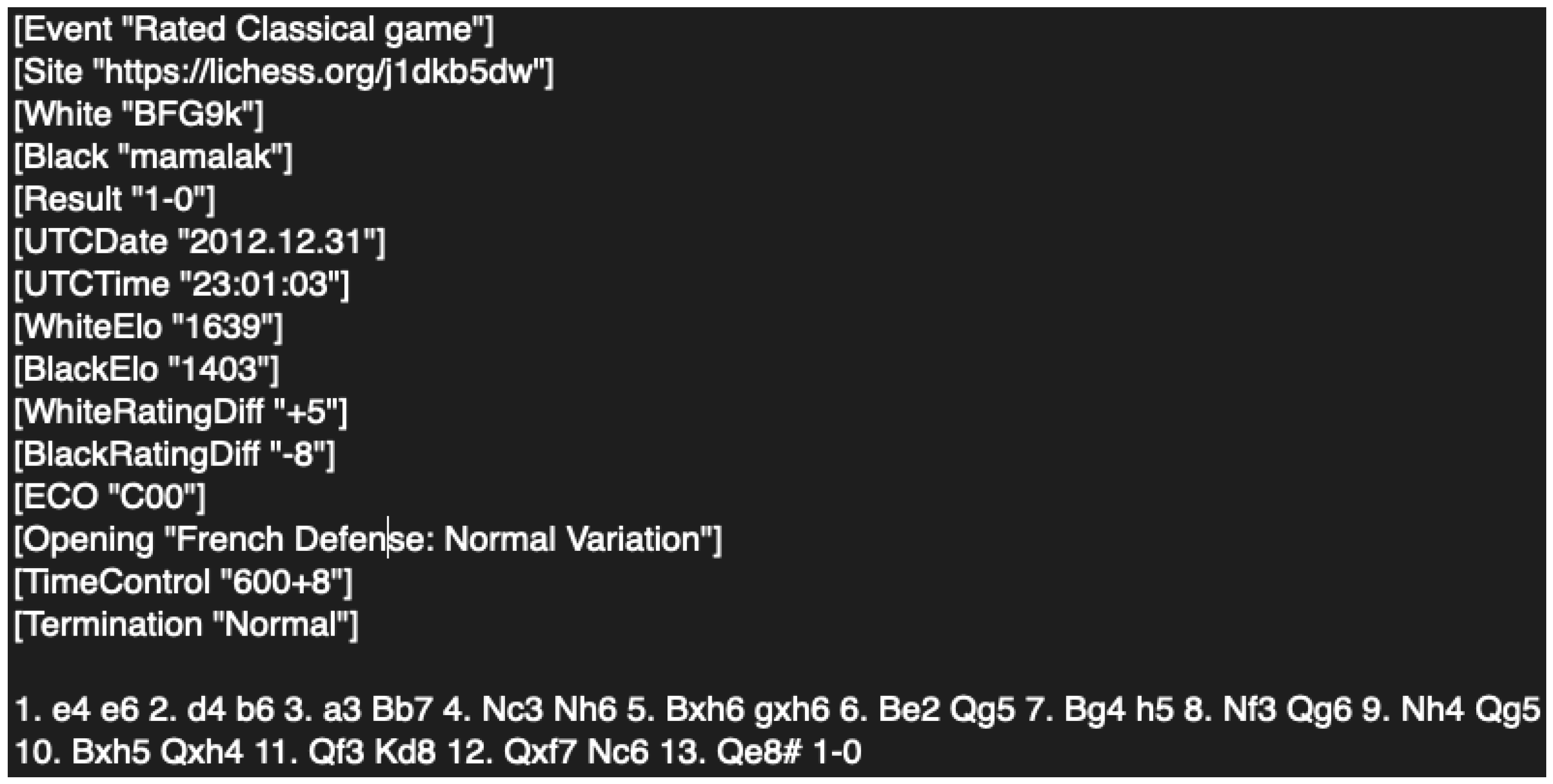
The raw data for the experiments were game data stored in Portable Game Notation (PGN) format [26], obtained from two sources. The primary source was the Lichess [9] database, which contains games played from 2013 until 2021. The second data set was sourced from the FICS [10] database, and we used games from 2019, as it contained the highest number of games. Figure 2 shows an example of a chess game recorded in PGN format. Altogether, we collected over one billion match data records from human players. In order to process such a large amount of data, we introduced several novel procedures to turn the match records into payoff matrices.
The first processing step was to extract the required attributes from the data of every game. These include the outcome of the game (to create the payoff matrix) and the Elo ratings of both players (as a measure of transitive strength).
The second step concerned the number of games taken from the whole Lichess database. As of 2021, the Lichess database contains a total of more than 2 billion games hosted from 2013. Therefore, sampling was required. Games were sampled uniformly across every month and year, where the number of games sampled every month was 120,000 as, for January of 2013, the database contains only a little more than 120,000 games. To avoid the influence of having a different number of points from each month, the number of games sampled per month was, thus, kept constant. In earlier years, sampling uniformly across a month was trivial, as games from an entire month could be loaded into a single data structure. However, for months in later years, the number of games in any given month could reach as many as 10 million. Therefore, a two-stage sampling method was required, as shown in Algorithm 1.
| Algorithm 1: Two-Stage Uniform Sampling. |
 |
Algorithm 1 can be proven to sample uniformly from U; that is, the probability of any object in U being sampled into F is . The proof is given in Appendix C. Note that, for FICS, the number of games in every month was relatively small, such that the database could be sampled directly.
The third processing step concerned discretisation of the whole strategy space to create a skew-symmetric payoff matrix representing the symmetric NF game. For this purpose, a single game outcome should represent the two participants playing two matches, with both participants playing black and white pieces once. We refer to such match-up as a two-way match-up. A single strategy, in the naïve sense, would thus be a combination of one contingency plan (as defined in Definition 4) if the player plays the white pieces with another one where the same player plays the black pieces. However, such a naïve interpretation of strategy would result in a very large strategy space. Therefore, we discretised the strategy space along the transitive dimension. As we used human games, we utilised the Elo rating of the corresponding players to measure the transitive strength. Therefore, given a pair of Elo ratings and , the game where the white player is of rating and the black player is of rating , and then another game where the black player is of rating and the white player is of rating , corresponds to a single two-way match-up. Discretisation was conducted by binning the Elo ratings such that, given two bins a and b, any two-way match-up where one player’s rating falls into a and the other player’s rating falls into b was treated as a two-way match-up between a and b. The resulting payoff matrix of an NF game is, thus, the outcomes of all two-way match-ups between every possible pair of bins. As two-way match-ups were considered, the resulting payoff matrices were skew-symmetric.
However, when searching for the corresponding two-way match-up between two bins of rating in the data set, there could either be multiple games or no games corresponding to this match-up. Consider a match-up between one bin and another bin . To fill in the corresponding entry of the matrix, a representative score for each case is first calculated. Let denote the representative score for the match-up where the white player’s rating is within a and the black player’s rating is within b, and denote the other direction. For the sake of argument, consider finding . As games are found for bin a against b, scores must be expressed from the perspective of a. The convention used in this paper is 1, 0, and for a win, draw, and loss, respectively. This convention ensures that the entries of the resulting payoff matrix are skew-symmetric. In the case where there are multiple games where the white player’s rating falls in a and black player’s rating falls in b, the representative score is then taken to be the average score from all these games. On the other hand, if there are no such games, the representative score is taken to be the expected score predicted from the Elo rating; that is,
where is the expected score of bin a against bin b, and is computed using Equation (2), by setting k as , , and . As this score is predicted using the Elo rating, it is indifferent towards whether the player is playing black or white pieces. After computing the representative score for both cases, the corresponding entry in the payoff matrix for the two-way match-up between bin a and b is simply the average of the representative score of both cases (i.e., ). The payoff matrix construction procedure is summarised in Algorithm 2.
In Algorithm 2, collects all games in D where the white player’s rating W is and the black player’s rating B is . Av averages game scores from the perspective of the white player (i.e., the score is 1, 0, if the white player wins, draws, or losses, respectively). Finally, in computing following Equation (2), and in the equation follow from the and computed in the previous line in the algorithm.
| Algorithm 2: Chess Payoff Matrix Construction. |
 |
3.3.2. Nash Clustering
Having constructed the payoff matrix in Section 3.3.1, we can now proceed with non-transitivity quantification. The first method of quantifying non-transitivity is through Nash Clustering [5]. Nash Clustering is derived from the layered game geometry, which states that the strategy space of a game can be clustered into an ordered list of layers such that any strategy in preceding layers is strictly better than any strategy in the succeeding layers. A game where the strategy space can be clustered in this way is known as a layered finite game of skill.
Definition 5.
A two-player zero-sum symmetric game is defined as a k-layered finite game of skill if the strategy space of each player can be factored into k layers , where , , , such that , , , and satisfying , , , .
A consequence of Definition 5 is that strategies in preceding layers would have a higher win-rate than those in succeeding layers. For any strategy , the corresponding win-rate is
Therefore, if we define the transitive strength of a layer to be the average win-rate of the strategies within that layer, the transitive strength of the layers would be ordered in descending order. Hence, intuitively, one can see the k-layered finite game of skill geometry as separating the transitive and non-transitive components of the strategy space. The non-transitivity is contained within each layer, whereas the transitivity variation happens across layers. It is, thus, intuitive to use the layer sizes as a measure of non-transitivity.
Furthermore, in Definition 5, the layer size increases monotonically up to a certain layer, from which it then decreases monotonically. Thus, when the transitive strength of each layer is plotted against its size, a two-dimensional spinning top structure would be observed if the change in size is strictly monotonic and . It is also for this reason that [5] named this geometry the spinning top geometry.
For every finite game, while there always exists for which the game is a k-layered finite game of skill, a value of does not always exist for any game; furthermore, the layered geometry is not useful if . Therefore, a relaxation to the k-layered geometry is required. In this alternative, a layer is only required to be “overall better” than the succeeding layers; however, it is not necessary that every strategy in a given layer beats every strategy in any succeeding layers. Such a layer structure was obtained through Nash Clustering.
Let , where , denote the symmetric NE of a two-player zero-sum symmetric game, in which both players are restricted to only the strategies in X, and is the payoff matrix from the perspective of player 1. Furthermore, let denote the set of pure strategies that are in support of the symmetric NE. Finally, let the set notation denote the set A excluding the elements that are in set B.
Definition 6.
Nash Clustering of a finite two-player zero-sum symmetric game produces a set of clusters C, defined as
Furthermore, to ensure that the Nash Clustering procedure is unique, we use the maximum entropy NE in Equation 1. Following Nash Clustering, the measure of non-transitivity would, thus, be the size or number of strategies in each cluster.
We then applied the Relative Population Performance (RPP) [27] to determine whether a layer or cluster is overall better than another cluster. Given two Nash clusters and , is overall better or wins against if . When using the RPP as a relative cluster performance measure, the requirement that any given cluster is overall better than any succeeding clusters proves to hold [5]. Following this, one can then use the fraction of clusters beaten, or win-rate, defined in Equation 6, as the measure of transitive strength of each cluster:
where I is the indicator function. We refer to the above win-rate as the RPP win-rate. Using the RPP win-rate as the measure of transitive strength of a Nash cluster guarantees that the transitive strength of Nash clusters are arranged in descending order.
Theorem 2.
Let C be the Nash Clustering of a two-player zero-sum symmetric game. Then, .
Proof.
Let C be the Nash Clustering of a two-player zero-sum symmetric game. Let where , . Let and . Using the fact that , as proven in [5], and . As , therefore, and since and , then . □
However, working with real data allowed us to use an alternative measure of transitive strength. We used the average Elo rating in Equation (2) of the pure strategies inside each Nash cluster to measure the transitive strength of the cluster. Specifically, given the payoff matrix from Section 3.3.1, each pure strategy corresponds to an Elo rating bin, and the transitive strength of a Nash cluster is therefore taken to be the average Elo rating of the bins inside that cluster. Let be a Nash cluster, be the integer indices of the pure strategies in support of , and be the bins used when constructing the payoff matrix, where each bin has lower and upper bounds , such that the bins corresponding to are . The average Elo rating of the Nash cluster is defined as
Given the average Elo rating against the cluster size for every Nash cluster, the final step would be to fit a curve to illustrate the spinning top geometry. For this purpose, we fitted an affine-transformed skewed normal distribution by minimising the Mean Squared Error (MSE). This completed the procedure of Nash Clustering using the average Elo rating as the measure of transitive strength.
In addition to using the average Elo rating, we also investigated the use of win-rates as a measure of transitive strength, as defined in Equation (6). However, instead of using the RPP to define the relative performance between clusters, we used a more efficient metric that achieves the same result when applied to Nash clusters. We refer to this metric as the Nash Population Performance (NPP).
Definition 7.
Let be the Nash Clustering of a two-player zero-sum symmetric game with payoff matrix . , where for and .
Using NPP also satisfies the requirement that any cluster is overall better than the succeeding clusters.
Theorem 3.
Let C be the Nash Clustering of a two-player zero-sum symmetric game. Then, , , and , .
The proof of Theorem 3 is given in Appendix C.
Theorem 3 suggests that applying the NPP to compute Equation (6) instead of the RPP would result in an identical win-rate for any Nash cluster, and the descending win-rate guarantee is preserved. Using the NPP is more efficient as, in Definition 7, for any Nash cluster is the corresponding NE solved during Nash Clustering to obtain that cluster; however, this means that the NPP is more suitable as a relative performance measure of Nash clusters, but less so for general population of strategies. For the latter, the RPP would be more suitable.
3.3.3. Rock–Paper–Scissor Cycles
Intuitively, a possible second method to quantify non-transitivity is to measure the length of the longest cycle in the strategy space, as this stems directly from the definition of non-transitivity. A cycle is defined as the sequence of strategies that starts and ends with the same strategy, where any strategy beats the immediate subsequent strategy in the sequence. However, calculating the length of the longest cycle in a directed graph is well-known to be NP-hard [28]. Therefore, we used the number of cycles of length three (i.e., rock–paper–scissor or RPS cycles) passing through every pure strategy as a proxy to quantify non-transitivity.
To obtain the number of RPS cycles passing through each pure strategy, an adjacency matrix is first formed from the payoff matrix. Letting the payoff matrix from Section 3.3.1 be , the adjacency matrix can be written as , where if , and 0 otherwise.
Theorem 4.
For an adjacency matrix where if there exists a directed path from node to node , the number of paths of length k that start from node and end on node is given by , where the length is defined as the number of edges.
The proof of Theorem 4 can be found in Appendix C. By Theorem 4, the number of RPS cycles passing through a strategy can thus be found by taking the diagonal of . Note that this does not apply to cycles with length of more than three, as the diagonal element of would include cycles with repeated nodes.
Finally, the measures of transitive strength used in this method are identical to those applied in Section 3.3.2, but applied to single strategies instead of clusters. This, therefore, completes the quantification of non-transitivity by counting RPS Cycles.
3.4. Relationships between Existing Rating Systems
As mentioned in Section 2, there are various chess player rating systems throughout the world, each of which is only valid for the pool of players over which the system is defined. As we used game data from Lichess and FICS to perform non-transitivity quantification, the results are therefore not directly applicable to different rating systems, such as USCF and FIDE. An investigation into the mappings between these rating systems is, thus, required.
We conducted a short experiment to obtain mappings between the rating systems of Lichess, USCF, and FIDE. The data set for this experiment was obtained from ChessGoals [29], which consisted of player ratings from four sites: Chess.com [30], FIDE, USCF, and Lichess.
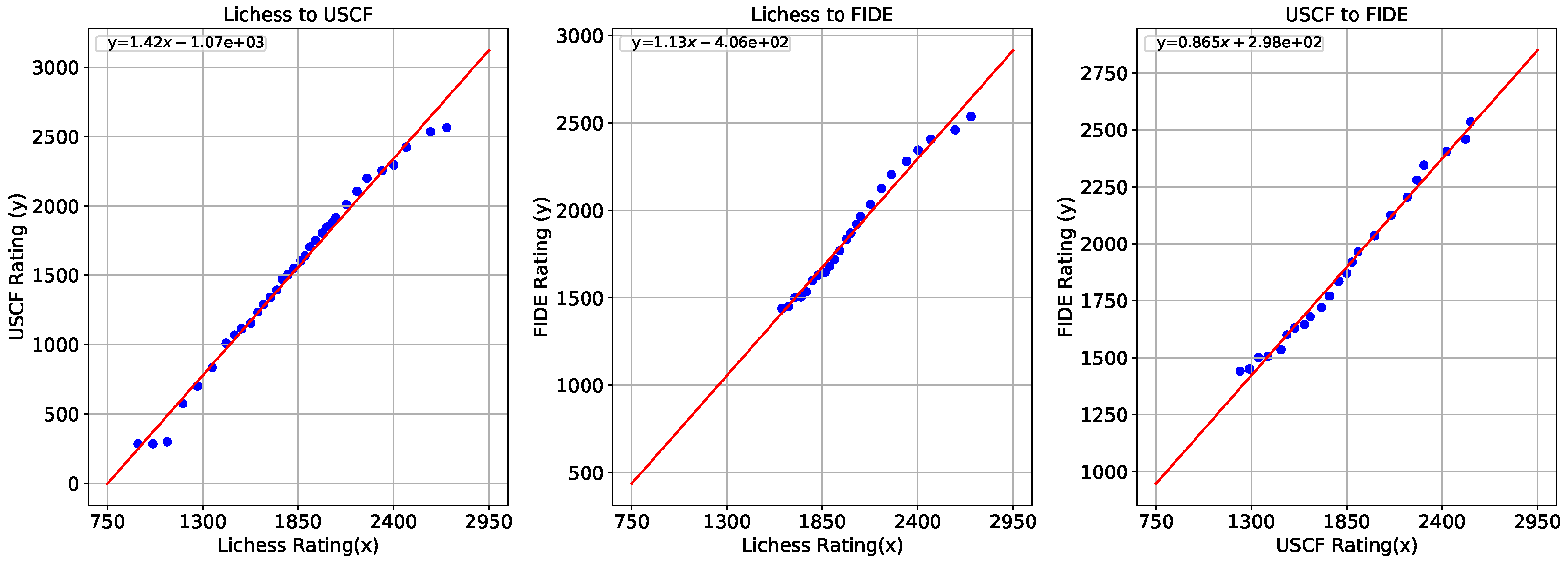
To investigate the mappings, we created three plots representing the mappings between pairs of rating systems: Lichess to USCF, Lichess to FIDE, and USCF to FIDE. A linear model was then fitted for each plot by MSE minimisation.
3.5. Implications of Non-Transitivity on Learning
Based on the discovered geometry, we also investigated the impact of non-transitivity on multi-agent reinforcement learning (MARL) [31]. Specifically, we designed experiments to verify the influence of non-transitivity on a particular type of MARL algorithm: Population-based learning [32,33,34,35]. This is a technique that underpins much of the existing empirical success in developing game AIs [36,37]. In fact, for simulated strategies [5], it has been found that, if the spinning top geometry exists in a strategy space, then the larger the non-transitivity of the game, in terms of layer size (for a k-layered geometry) or Nash cluster size (for Nash Clustering), the larger the population size required for methods such as fixed-memory Fictitious Play to converge. We attempted to verify whether the above conclusion still holds when real-world data are used instead. Furthermore, observing the above convergence trend with respect to the starting population size provides even stronger evidence for the existence of the spinning top geometry in the strategy space of real-world chess.
As a proxy for a population-based training method, fixed-memory Fictitious Play starts with a population (or set) of pure strategies , of fixed size k. The starting pure strategies in are chosen to be the k weakest pure strategies, based on the win-rate against other pure strategies, as shown in Equation (4). At every iteration t of the fictitious play, the oldest pure strategy in the population is replaced with a pure strategy that is not in . The replacement strategy is required to beat all the strategies in the current population on average; that is, suppose that is the replacement strategy at iteration t. Then, it is required that . If there are multiple strategies satisfying this condition, then the selected strategy is the one with the lowest win-rate (i.e., , where ).
To measure the performance at every iteration of the fictitious play, we used the expected average payoff of the population at that iteration. Suppose that, at any iteration t, the probability allocation over the population , which is of size k, is . Given the payoff matrix of size , the performance of the population , , is written as:
where is the pure strategy corresponding to the column of . The complete fixed-memory Fictitious Play is summarised in Algorithm 3.
| Algorithm 3: Fixed-Memory Fictitious Play. |
 |
In Algorithm 3, for any list a and b where b contains integers, the notation means taking all elements in a at index positions denoted by the elements in b, in the order that the integers are arranged in b. Furthermore, argsort(a) returns a list of indices d, such that is a sorted in ascending order. Additionally, “compute win rate” in Algorithm 3 is the function described in Algorithm 4. In this function, for any matrix M, the notation means taking all rows and columns of M only at positions indicated by the elements in b. Finally, size(a) returns the number of elements in the list a.
Algorithm 4 is used to compute the training performance of a population of k strategies at every round of fictitious play, following Equation (8). The convergence of fixed-memory Fictitious Play in Algorithm 3 is not dependent on the metric used to measure performance at every round, as convergence of the fictitious play means there are no more valid replacement strategies (i.e., ). Hence, we chose to use Algorithm 4 to measure the performance at every step, due to its simplicity.
| Algorithm 4: Compute Win Rate. |
 |
3.6. Link to Human Skill Progression
In Section 3.5, we hypothesised that non-transitivity has implications on the performance improvement of AI agents during training. On the other hand, one of the most common issue faced by human chess players is the phenomenon of becoming stuck at a certain Elo rating [38,39,40]. Having performed experiments using real data, we also investigated whether non-transitivity has implications for a human player’s skill or rating progression. In particular, we investigated whether a link exists between the non-transitivity of the strategy space of real-world chess to the phenomenon of players getting stuck at certain Elo ratings. This was conducted by comparing the histogram of player ratings every year using the data from Section 3.3.1, with the corresponding Nash Clustering plot.
3.7. Algorithm Hyperparameter Considerations
Algorithms 2 and 3, introduced in Section 3.3.1 and Section 3.5, respectively, contain hyperparameters, and the choice of values for these hyperparameters merits further discussion.
In Algorithm 2, the hyperparameter is the size of the payoff matrix m. The time complexity of Algorithm 2 with respect to the payoff matrix dimension m is . Therefore, having a large payoff matrix would severely slow down the payoff matrix construction. However, using a small payoff matrix would result in more data being unused. Algorithm 2 constructs a payoff matrix that is skew-symmetric and, so, the diagonal of the payoff matrix is be 0. As m gets smaller, the bin widths get wider and, thus, a wider range of Elo ratings are absorbed into a single bin. As a result, the non-diagonal elements of the matrix would correspond to two-way match-ups between two players with a more significant difference in Elo ratings, which is less likely to be present in the actual data, as players are typically matched with other players having similar Elo ratings. Therefore, a majority of the non-diagonal elements of the matrix will be filled using the Elo formula in Equation (3), instead of real data, which effectively turns the game into a purely transitive Elo game [5]. This leads to us not being able to observe the spinning top geometry in the strategy space occupied by real-world strategies. In our experiments, we used an m of 1500, as this was sufficiently large to demonstrate the existence of the spinning top geometry, while keeping the payoff matrix construction reasonably fast.
In Algorithm 3, the hyperparameters are the population size k and the number of rounds n. The time complexity of Algorithm 3 is more affected by the number of rounds n, on the order of . While it grows slower than the time complexity of Algorithm 2 with respect to m, it is still desirable to keep n relatively small, as fixed-memory Fictitious Play would have to be carried out for a number of population sizes. However, n should be large enough to demonstrate the convergence behaviour of the training process, if any. From our experiments, we found that 2000 rounds were sufficient for this purpose. The choice of population sizes is elaborated more in Section 4.3.
4. Results and Discussions
4.1. Non-Transitivity Quantification
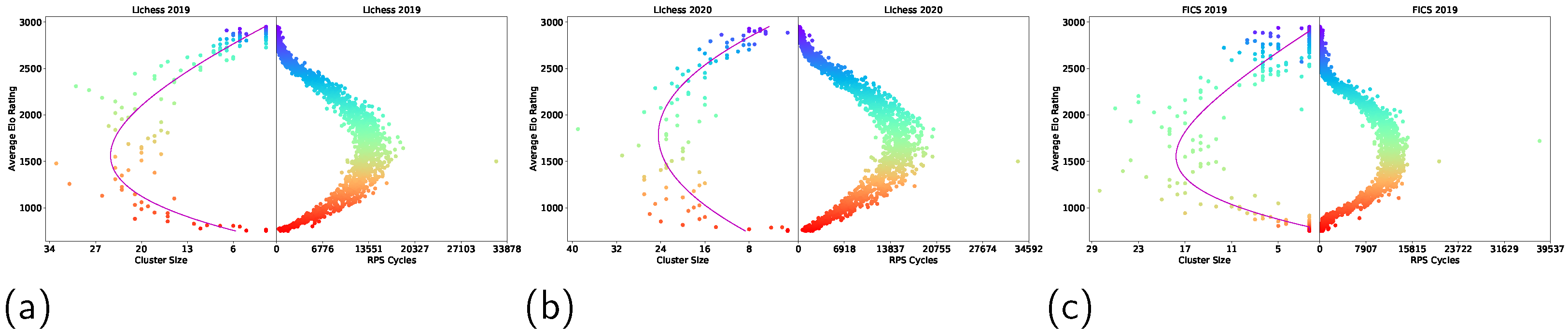
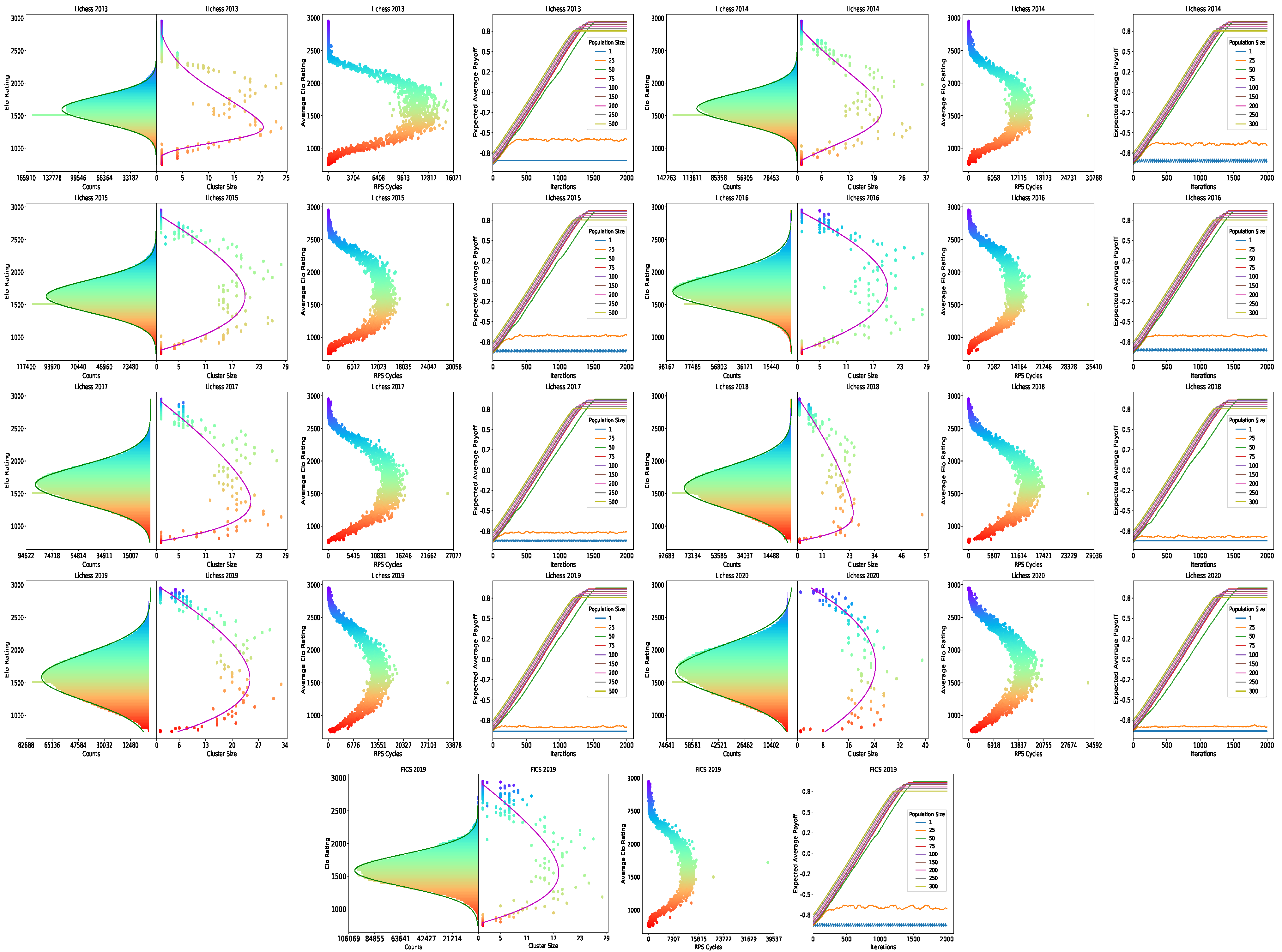
Following Section 3.3.2 and Section 3.3.3, non-transitivity quantification was carried out on Lichess game data from 2013 to 2020, and FICS 2019 data, using the average Elo rating as a measure of transitive strength, and the Nash Cluster size and number of RPS cycles as measures of non-transitivity. The results are as shown in Figure 3.
Figure 3 and Figure A1 illustrate that the spinning top geometry was observed in both Nash Clustering and RPS Cycles plots, for all of the considered years. Furthermore, both the Nash cluster size and number of RPS cycles peaked at a similar Elo rating range (1300–1700) for all of the years. This provides comprehensive evidence that the strategies adopted in real-world games do not vary throughout the years or from one online platform to another, and that the non-transitivity of real-world strategies is highest in the Elo rating range of 1300–1700.
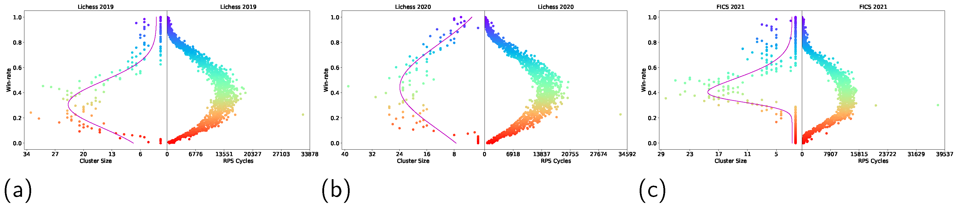
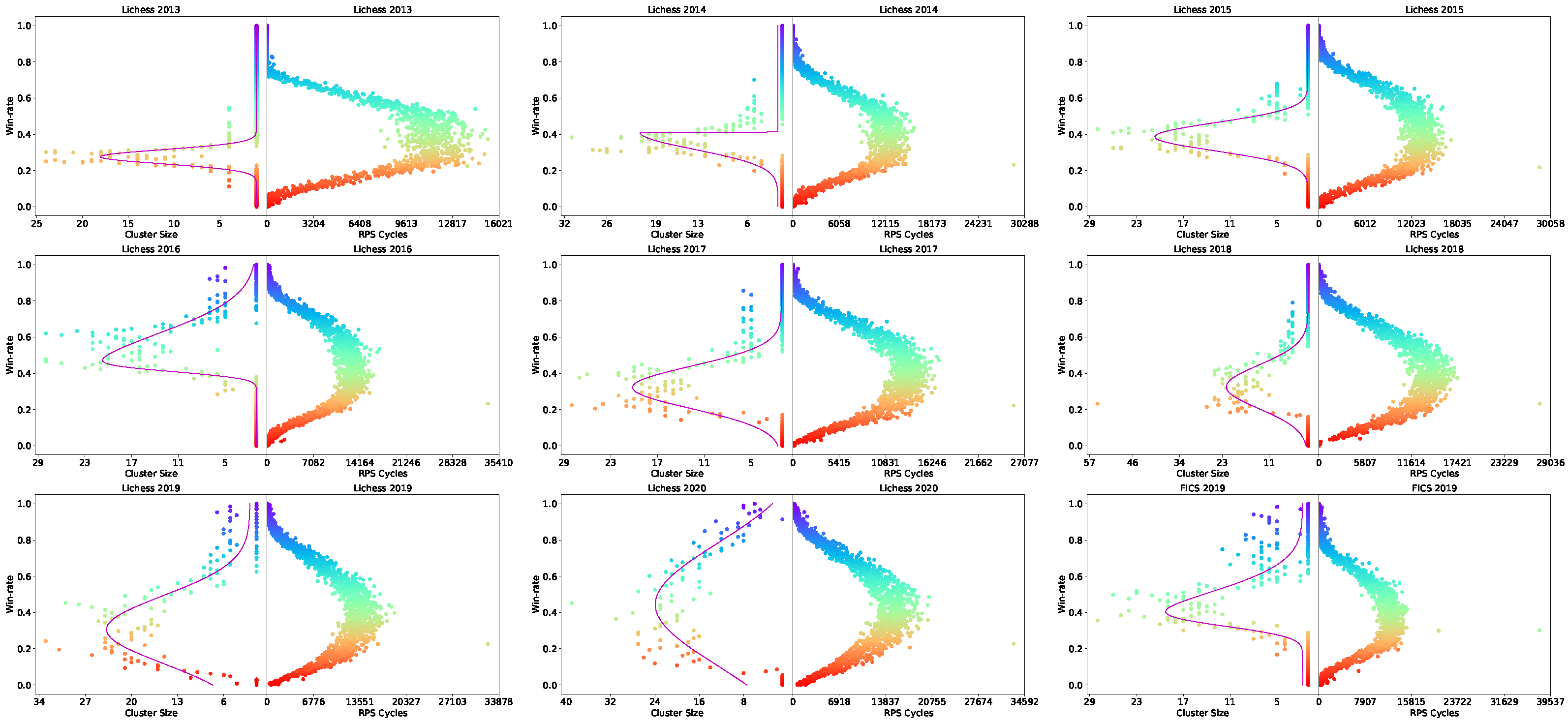
Furthermore, as stated in Section 3.3.2 and Section 3.3.3, we also performed the above non-transitivity quantifications using win-rates as a measure of transitive strength, as it provides stronger evidence for the existence of the spinning top geometry should this geometry persist. The results are shown in Figure 4.
Despite using a different measure of transitive strength in Figure 4 and Figure A2, the results show that the spinning top geometry still persisted for all the years. Not only does this provide stronger evidence for the existence of a spinning top geometry within the real-world strategy space of chess, it also indicates that measuring non-transitivity using both Nash Clustering and RPS Cycles is agnostic towards the measure of transitive strength used.
4.2. Relationships between Existing Rating Systems
Following Section 3.4, we fitted three Linear Regression models representing the mappings between three rating systems discussed in that section; namely, Lichess, USCF, and FIDE rating systems. The results are shown in Figure 5.
Figure 5 shows that the relationships between Lichess, USCF, and FIDE ratings were largely linear and monotonically increasing, and that the linear models fit the data sufficiently well. As the mappings between the rating systems were monotonically increasing, the spinning top geometry observed in Figure 3 is expected to still hold when mapped to USCF or FIDE rating systems. This is as the relative ordering of the Nash clusters or pure strategies based on Elo rating will be preserved. Therefore, our results are directly applicable to different rating systems.
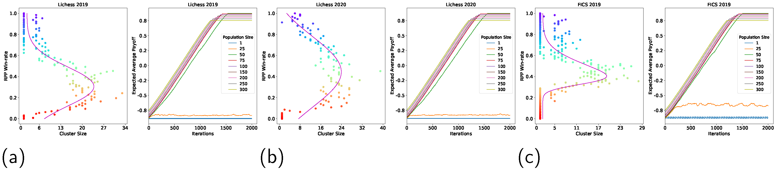
4.3. Implications of Non-Transitivity on Learning
Following Section 3.5, we conducted fixed-memory Fictitious Play, as described in Algorithm 3, using payoff matrices constructed following Section 3.3.1. Fictitious Play was carried out with population sizes of 1, 25, 50, 75, 100, 150, 200, 250, and 300, in order to demonstrate the effect of non-transitivity, in terms of Nash Cluster sizes, on the minimum population size needed for training to converge. These values were chosen by comparing the games in [5] with similar Nash Cluster sizes. Figure 3 and Figure A1 show that the largest Nash cluster sizes were in the range of 25 to slightly above 50. In [5], the game Hex [41] had similar Nash cluster sizes, with the largest size being slightly less than 50. For this game, [5] used population sizes of 1, 25, 50, 75, 100, 150, 200, 250, and 300; thus, we used these values in our experiments as well. The results are shown in Figure 6.
Figure 6 and Figure A1 show that the training process converged for all cases, provided that the population size was 50 or above. This is because the Nash cluster sizes are never much larger than 50 and, therefore, a population size of 50 ensures good coverage of the Nash clusters at any transitive strength. Such convergence behaviour also provides additional evidence that the spinning top geometry is present in the strategy space of real-world chess.
It should be noted, however, that the minimum population size needed for training to converge does not always correspond to the largest Nash cluster size, for which there are two contributing factors. The first factor is that covering a full Nash cluster (i.e., having a full Nash cluster in the population at some iteration) only guarantees the replacement strategy at that iteration to be from a cluster of greater transitive strength than the covered cluster. There are no guarantees that this causes subsequent iterations to cover Nash clusters of increasing transitive strength. The second factor is that the convergence guarantee is with respect to the k-layered game of skill geometry defined in Definition 5. As Nash Clustering is a relaxation of this geometry, covering a full Nash cluster does not guarantee that the minimal population size requirement will be satisfied.
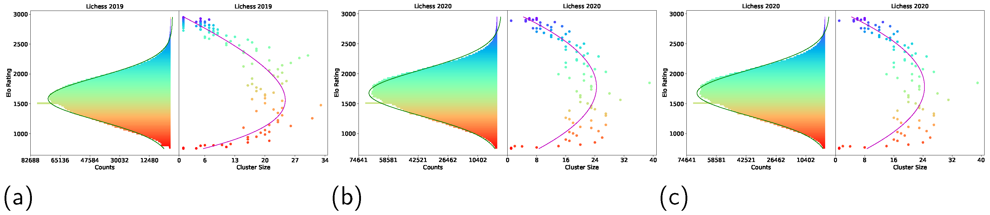
4.4. Link to Human Skill Progression
Following Section 3.6, we plotted the histogram of player ratings alongside the corresponding Nash Clustering plots for comparison. The results are shown in Figure 7.
Figure 7 and Figure A1 shows that the peaks of the histograms and the bulk of the data consistently fell in the 1300–1700 Elo rating range, which matches with the range of Elo ratings in which players tend to get stuck, as stated in [38,39,40], suggesting that players tend to get stuck in this range. Furthermore, the peaks of the histograms coincided with the peak of the fitted skewed normal curve on the Nash Clustering plots. This implies that high non-transitivity in the 1300 to 1700 rating range is one potential cause of players getting stuck in this range.
A plausible explanation is that, in the 1300–1700 Elo rating range, there exist a lot of RPS cycles (as can be seen from Figure 3), which means there exist a large number of counter-strategies. Therefore, to improve from this Elo rating range, players need to learn how to win against many strategies; for example, by dedicating more effort toward learning diverse opening tactics. Otherwise, their play-style may be at risk of being countered by some strategies at that level. This is in contrast to ratings where non-transitivity is low. With a lower number of counter-strategies, it is arguably easier to improve, as there are relatively fewer strategies to adapt towards.
5. Conclusions and Future Work
The goal of this paper was to measure the non-transitivity of chess games and investigate the potential implications for training effective AI agents, as well as those for human skill progression. Our work is novel in the sense that we, for the first time, profiled the geometry of the strategy space based on real-world data from human players. This, in turn, prompted the discovery of the spinning top geometry, which has only been previously observed for AI-generated strategies; more importantly, we uncovered the relationship between the degree of non-transitivity and the progression of human skill in playing chess. Additionally, the discovered relationship also indicates that, in order to overcome the non-transitivity in the strategy space, it is imperative to maintain large population sizes when applying population-based methods in training AIs. Throughout our analysis, we managed to tackle several practical challenges. For example, despite the variation in Elo rating systems for chess, we introduced effective mappings between those rating systems, which enables direct translation of our findings across different rating systems.
Finally, there are several avenues for possible improvements, which we leave for future work:
- In Section 3.3.1, missing data between match-ups of bins are filled using Elo formulas; that is, Equations (2) and (3). However, the Lichess ratings use the Glicko-2 system [20], which has a slightly different win probability formula that also considers the rating deviation and volatility of the rating. Therefore, a possible improvement would be to additionally collect the rating deviation and volatility of the players in every game, and apply the Glicko-2 predictive formula to compute the win probability, instead of Equation (2).
- Non-transitivity analysis could also be carried out using other online chess platforms, such as Chess.com [30], in order to provide more comprehensive evidence on the spinning top geometry of the real-world strategy space. Furthermore, the non-transitivity analysis could also be carried out using real-world data on other, more complex, zero-sum games, such as Go, DOTA and StarCraft.
- Other links between non-transitivity and human progression can be investigated. One possible method would be to monitor player rating progression from the start of their progress to when they achieve a sufficiently high rating in a chess platform, such as Lichess. Their rating progression can then be compared to the non-transitivity at that rating and in that year. However, player rating progression is typically not available on online chess platforms and, thus, would require monitoring player progress over an extended period of time.
Author Contributions
Conceptualization, R.S.; methodology, R.S.; software, R.S.; validation, R.S.; formal analysis, R.S.; investigation, R.S.; resources, R.S.; data curation, R.S.; writing—original draft preparation, R.S.; writing—review and editing, R.S. and Y.Y.; supervision, Y.Y. and J.W.; project administration, Y.Y. and J.W. All authors have read and agreed to the published version of the manuscript.
Funding
This research received no external funding.
Institutional Review Board Statement
Not applicable.
Informed Consent Statement
Not applicable.
Data Availability Statement
The python codes to replicate the experiments in this paper are available at https://anonymous.4open.science/r/MSc-Thesis-8543 (accessed on 13 March 2022). README.md contains all the instructions to run the codes. Finally, the data sets can be downloaded from https://database.lichess.org/ (accessed on 13 March 2022) for Lichess and https://www.ficsgames.org/ (accessed on 13 March 2022) for FICS.
Conflicts of Interest
The authors declare no conflict of interest.
Appendix A. Additional Results
Figure A1.
Histogram of player Elo ratings (first of each plot), Nash Clustering (second of each plot), RPS Cycles (third of each plot), and fixed-memory Fictitious Play (fourth of each plot) on Lichess 2013–2020 and FICS 2019 data.
Figure A1.
Histogram of player Elo ratings (first of each plot), Nash Clustering (second of each plot), RPS Cycles (third of each plot), and fixed-memory Fictitious Play (fourth of each plot) on Lichess 2013–2020 and FICS 2019 data.

Appendix B. Additional Results with Alternative Measure of Transitive Strength
Figure A2.
Measurements of Nash Clustering (left of each plot) and RPS Cycles (right of each plot) using win-rate as measure of transitive strength on Lichess 2013–2020 and FICS 2019 data.
Figure A2.
Measurements of Nash Clustering (left of each plot) and RPS Cycles (right of each plot) using win-rate as measure of transitive strength on Lichess 2013–2020 and FICS 2019 data.

Appendix C. Theorem Proofs
Theorem A1.
With Algorithm 1, the probability of any object in M being sampled into F is .
Proof.
For any object in U to end up in F, they must first get picked into G. As , , the probability that any object is sampled into G is . Then, given that they are in G, they must get sampled into F. The probability that this happens is . Hence, the probability that any object from U gets sampled into F is . □
Theorem A2.
Let C be the Nash Clustering of a two-player zero-sum symmetric game. Then, , and , .
Proof.
Let C be the Nash Clustering of a two-player zero-sum symmetric game with a payoff matrix of and strategy space for each of the two players. For any , let be the NE solved to obtain the cluster; that is, , where . As is restricted to exclude , therefore, would be all zeroes at the positions corresponding to all pure strategies . Let and be the payoff matrix of the game, but excluding the rows and columns that corresponds to the pure strategies in . Additionally, let denote the vector but removing all entries at positions corresponding to the pure strategies in . Hence, and . Furthermore, it is also true that for any , provided that the entries of at positions corresponding to pure strategies in are zeroes.
By definition of NE in [42], we have that and . Now, consider two clusters and , where and . By the first definition of NE earlier, , which implies and, thus, equivalently . Then, by the properties of skew-symmetric matrices, and, hence, ; that is, . Furthermore, by the second definition of NE earlier, , which implies and, thus, equivalently . Finally, using the property of skew-symmetric matrices again, ; that is, . □
Theorem A3.
For an adjacency matrix where , if there exists a directed path from node to node , the number of paths of length k that starts from node and ends on node is given by , where the length is defined as the number of edges in that path.
Proof.
By induction, the base case is when . A path from node to node of length 1 is simply a direct edge connecting to . The presence of such an edge is indicated by , which follows from the definition of adjacency matrix, thereby proving the base case. The inductive step is then to prove that if is the number of paths of length k from node to for some , then is the number of paths of length from node to . This follows from matrix multiplication. Let . Then, . The inner multiplicative term of the sum will only be non-zero if both and are non-zero, indicating that there exists a path of length k from node to some node and, then, a direct edge from that node to . This forms a path of length from node to . Therefore, counts the number of paths of length from node to , proving the inductive hypothesis. □
References
- Ensmenger, N. Is chess the drosophila of artificial intelligence? A social history of an algorithm. Soc. Stud. Sci. 2012, 42, 5–30. [Google Scholar] [CrossRef] [PubMed] [Green Version]
- Shannon, C.E. XXII. Programming a computer for playing chess. Lond. Edinb. Dublin Philos. Mag. J. Sci. 1950, 41, 256–275. [Google Scholar] [CrossRef]
- Campbell, M.; Hoane, A.J., Jr.; Hsu, F.h. Deep blue. Artif. Intell. 2002, 134, 57–83. [Google Scholar] [CrossRef] [Green Version]
- Silver, D.; Hubert, T.; Schrittwieser, J.; Antonoglou, I.; Lai, M.; Guez, A.; Lanctot, M.; Sifre, L.; Kumaran, D.; Graepel, T.; et al. Mastering chess and shogi by self-play with a general reinforcement learning algorithm. arXiv 2017, arXiv:1712.01815. [Google Scholar]
- Czarnecki, W.M.; Gidel, G.; Tracey, B.; Tuyls, K.; Omidshafiei, S.; Balduzzi, D.; Jaderberg, M. Real World Games Look Like Spinning Tops. In Proceedings of the Advances in Neural Information Processing Systems, Vancouver, BC, Canada, 6–12 December 2020. [Google Scholar]
- Nash, J. Non-cooperative games. Ann. Math. 1951, 54, 286–295. [Google Scholar] [CrossRef]
- McIlroy-Young, R.; Sen, S.; Kleinberg, J.; Anderson, A. Aligning Superhuman AI with Human Behavior: Chess as a Model System. In Proceedings of the 26th ACM SIGKDD International Conference on Knowledge Discovery & Data Mining, Virtual Event. CA, USA, 6–10 July 2020; pp. 1677–1687. [Google Scholar]
- Romstad, T.; Costalba, M.; Kiiski, J.; Linscott, G. Stockfish: A strong open source chess engine. 2017. Open Source. Available online: https://stockfishchess.org (accessed on 18 August 2021).
- Lichess. About lichess.org. Available online: https://lichess.org/about (accessed on 16 August 2021).
- FICS. FICS Free Internet Chess Server. Available online: https://www.freechess.org/ (accessed on 16 August 2021).
- Yang, Y.; Luo, J.; Wen, Y.; Slumbers, O.; Graves, D.; Bou Ammar, H.; Wang, J.; Taylor, M.E. Diverse Auto-Curriculum is Critical for Successful Real-World Multiagent Learning Systems. In Proceedings of the 20th International Conference on Autonomous Agents and MultiAgent Systems, London, UK, 3–7 May 2021; pp. 51–56. [Google Scholar]
- Russell, S.; Norvig, P. Artificial Intelligence: A Modern Approach; Prentice Hall: Englewood Cliffs, NJ, USA, 2002. [Google Scholar]
- Chaslot, G.; Bakkes, S.; Szita, I.; Spronck, P. Monte-Carlo Tree Search: A New Framework for Game AI. AIIDE 2008, 8, 216–217. [Google Scholar]
- Vinyals, O.; Babuschkin, I.; Czarnecki, W.M.; Mathieu, M.; Dudzik, A.; Chung, J.; Choi, D.H.; Powell, R.; Ewalds, T.; Georgiev, P.; et al. Grandmaster level in StarCraft II using multi-agent reinforcement learning. Nature 2019, 575, 350–354. [Google Scholar] [CrossRef] [PubMed]
- International Chess Federation. FIDE Charter, Art. 1 FIDE—Name, Legal Status and Seat. Available online: https://handbook.fide.com/files/handbook/FIDECharter2020.pdf (accessed on 16 August 2021).
- United States Chess Federation. About US Chess Federation. Available online: https://new.uschess.org/about (accessed on 16 August 2021).
- Glickman, M.E.; Doan, T. The US Chess Rating System. 2020. Available online: https://new.uschess.org/sites/default/files/media/documents/the-us-chess-rating-system-revised-september-2020.pdf (accessed on 18 August 2021).
- International Chess Federation. FIDE Handbook, B. Permanent Commissions/02. FIDE Rating Regulations (Qualification Commission)/FIDE Rating Regulations Effective from 1 July 2017 (with Amendments Effective from 1 February 2021). Available online: https://handbook.fide.com/chapter/B022017 (accessed on 20 August 2021).
- Glickman, M.E. The Glicko System; Boston University: Boston, MA, USA, 1995; Volume 16, pp. 16–17. [Google Scholar]
- Glickman, M.E. Example of the Glicko-2 System; Boston University: Boston, MA, USA, 2012; pp. 1–6. [Google Scholar]
- Deng, X.; Li, Y.; Mguni, D.H.; Wang, J.; Yang, Y. On the Complexity of Computing Markov Perfect Equilibrium in General-Sum Stochastic Games. arXiv 2021, arXiv:2109.01795. [Google Scholar]
- Balduzzi, D.; Tuyls, K.; Pérolat, J.; Graepel, T. Re-evaluating evaluation. In Proceedings of the NeurIPS; Neural Information Processing Systems Foundation, Inc.: Montréal, QC, Canada, 2018; pp. 3272–3283. [Google Scholar]
- Hart, S. Games in extensive and strategic forms. In Handbook of Game Theory with Economic Applications; Elsevier: Amsterdam, The Netherlands, 1992; Volume 1, pp. 19–40. [Google Scholar]
- Kuhn, H.W. Extensive games. In Lectures on the Theory of Games (AM-37); Princeton University Press: Princeton, NJ, USA, 2009; pp. 59–80. [Google Scholar]
- Elo, A.E. The Rating of Chessplayers, Past and Present; Arco Pub.: Nagoya, Japan, 1978. [Google Scholar]
- Edwards, S.J. Standard Portable Game Notation Specification and Implementation Guide. 1994. Available online: http://www.saremba.de/chessgml/standards/pgn/pgncomplete.htm (accessed on 10 August 2021).
- Balduzzi, D.; Garnelo, M.; Bachrach, Y.; Czarnecki, W.; Perolat, J.; Jaderberg, M.; Graepel, T. Open-ended learning in symmetric zero-sum games. In Proceedings of the International Conference on Machine Learning. PMLR, Long Beach, CA, USA, 9–15 June 2019; pp. 434–443. [Google Scholar]
- Björklund, A.; Husfeldt, T.; Khanna, S. Approximating longest directed paths and cycles. In Proceedings of the International Colloquium on Automata, Languages, and Programming, Turku, Finland, 12–16 July 2004; pp. 222–233. [Google Scholar]
- ChessGoals. Rating Comparison Database. 2021. Available online: https://chessgoals.com/rating-comparison/.
- Chess.com. About Chess.com. Available online: https://www.chess.com/about (accessed on 16 August 2021).
- Yang, Y.; Wang, J. An Overview of Multi-Agent Reinforcement Learning from Game Theoretical Perspective. arXiv 2020, arXiv:2011.00583. [Google Scholar]
- Lanctot, M.; Zambaldi, V.; Gruslys, A.; Lazaridou, A.; Tuyls, K.; Pérolat, J.; Silver, D.; Graepel, T. A unified game-theoretic approach to multiagent reinforcement learning. In Proceedings of the 31st International Conference on Neural Information Processing Systems, Long Beach, CA, USA, 4–9 December 2017; pp. 4193–4206. [Google Scholar]
- Perez-Nieves, N.; Yang, Y.; Slumbers, O.; Mguni, D.H.; Wen, Y.; Wang, J. Modelling Behavioural Diversity for Learning in Open-Ended Games. In Proceedings of the International Conference on Machine Learning, PMLR. Virtual, 18–24 July 2021; pp. 8514–8524. [Google Scholar]
- Liu, X.; Jia, H.; Wen, Y.; Yang, Y.; Hu, Y.; Chen, Y.; Fan, C.; Hu, Z. Unifying Behavioral and Response Diversity for Open-ended Learning in Zero-sum Games. arXiv 2021, arXiv:2106.04958. [Google Scholar]
- Dinh, L.C.; Yang, Y.; Tian, Z.; Nieves, N.P.; Slumbers, O.; Mguni, D.H.; Ammar, H.B.; Wang, J. Online Double Oracle. arXiv 2021, arXiv:2103.07780. [Google Scholar]
- Zhou, M.; Wan, Z.; Wang, H.; Wen, M.; Wu, R.; Wen, Y.; Yang, Y.; Zhang, W.; Wang, J. MALib: A Parallel Framework for Population-based Multi-agent Reinforcement Learning. arXiv 2021, arXiv:2106.07551. [Google Scholar]
- Lanctot, M.; Lockhart, E.; Lespiau, J.B.; Zambaldi, V.; Upadhyay, S.; Pérolat, J.; Srinivasan, S.; Timbers, F.; Tuyls, K.; Omidshafiei, S.; et al. OpenSpiel: A framework for reinforcement learning in games. arXiv 2019, arXiv:1908.09453. [Google Scholar]
- Chess.com. Stuck at the Same Rating for a Long Time. 2019; Available online: https://www.chess.com/forum/view/general/stuck-at-the-same-rating-for-a-long-time-1 (accessed on 16 August 2021).
- Lichess. My Friends Are Stuck at 1500–1600 How Long Will it Take Them to Get Up to 1700. 2021. Available online: https://lichess.org/forum/general-chess-discussion/my-friends-are-stuck-at-1500-1600-how-long-will-it-take-them-to-get-up-to-1700 (accessed on 13 March 2022).
- Lichess. Stuck at 1600 Rating. 2021. Available online: https://lichess.org/forum/general-chess-discussion/stuck-at-1600-rating (accessed on 13 March 2022).
- Hayward, R.B.; Toft, B. Hex, Inside and Out: The Full Story; CRC Press: Boca Raton, FL, USA, 2019. [Google Scholar]
- Daskalakis, C. Two-Player Zero-Sum Games and Linear Programming. 2011. Available online: http://people.csail.mit.edu/costis/6896sp10/lec2.pdf (accessed on 21 August 2021).
Figure 1.
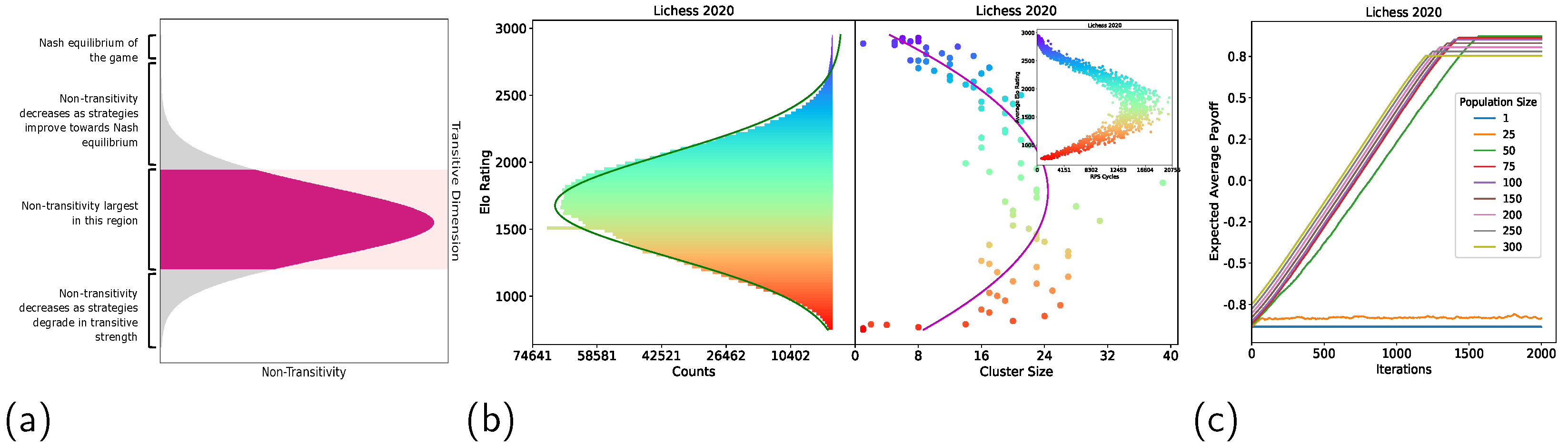
We justify the spinning top hypothesis represented by (a), which states that many real-world games—including chess—possess a strategy space with a spinning top geometry, where the radial axis represents the non-transitivity degree (e.g., A beats B, B beats C, and C beats A) and the upright axis represents the transitivity degree (e.g., A beats B, B beats C, and A beats C). We studied the geometric properties of chess based on one billion game records from human players. (b) shows the comparison between the histogram of Elo ratings (i.e., the transitivity degree) in Lichess 2020 (left) and the degree of non-transitivity at each Elo level (right), where the non-transitivity is measured by both the size of the Nash clusters and the number of rock–paper–scissor cycles (top-right corner). A skewed-normal curve is fitted to illustrate the non-transitivity profile, which verifies the spinning top hypothesis in (a). Specifically, the middle region of the transitive dimension is accompanied by a large degree of non-transitivity, which gradually diminishes as skill evolves towards high Elo ratings (upward) or degrades (downward). Notably, the peak of the Elo histogram lies between 1300 and 1700, a range where most human players get stuck. Furthermore, the peak of the non-transitivity curve coincides with the peak of the Elo histogram; this indicates a strong relationship between the difficulty of playing chess and the degree of non-transitivity. Our discovered geometry has important implications for learning. For example, our findings provide guidance to improve the Elo ratings of human players, especially in stages with high degrees of non-transitivity (e.g., by dedicating more efforts to learning diverse opening tactics). In (c), we show the performances of population-based training methods with different population sizes. A phase change in performance occurs when the population size increases; this justifies the necessity of maintaining large and diverse populations when training AI agents to solve chess.
Figure 1.
We justify the spinning top hypothesis represented by (a), which states that many real-world games—including chess—possess a strategy space with a spinning top geometry, where the radial axis represents the non-transitivity degree (e.g., A beats B, B beats C, and C beats A) and the upright axis represents the transitivity degree (e.g., A beats B, B beats C, and A beats C). We studied the geometric properties of chess based on one billion game records from human players. (b) shows the comparison between the histogram of Elo ratings (i.e., the transitivity degree) in Lichess 2020 (left) and the degree of non-transitivity at each Elo level (right), where the non-transitivity is measured by both the size of the Nash clusters and the number of rock–paper–scissor cycles (top-right corner). A skewed-normal curve is fitted to illustrate the non-transitivity profile, which verifies the spinning top hypothesis in (a). Specifically, the middle region of the transitive dimension is accompanied by a large degree of non-transitivity, which gradually diminishes as skill evolves towards high Elo ratings (upward) or degrades (downward). Notably, the peak of the Elo histogram lies between 1300 and 1700, a range where most human players get stuck. Furthermore, the peak of the non-transitivity curve coincides with the peak of the Elo histogram; this indicates a strong relationship between the difficulty of playing chess and the degree of non-transitivity. Our discovered geometry has important implications for learning. For example, our findings provide guidance to improve the Elo ratings of human players, especially in stages with high degrees of non-transitivity (e.g., by dedicating more efforts to learning diverse opening tactics). In (c), we show the performances of population-based training methods with different population sizes. A phase change in performance occurs when the population size increases; this justifies the necessity of maintaining large and diverse populations when training AI agents to solve chess.

Figure 2.
Lichess PGN format.

Figure 3.
Nash Clustering (left of each plot) and RPS Cycles (right of each plot) on Lichess 2019 (a), Lichess 2020 (b), and FICS 2019 (c). See Figure A1 in Appendix A for the full version of the results, which include Lichess 2013–2020 and FICS 2019.
Figure 3.
Nash Clustering (left of each plot) and RPS Cycles (right of each plot) on Lichess 2019 (a), Lichess 2020 (b), and FICS 2019 (c). See Figure A1 in Appendix A for the full version of the results, which include Lichess 2013–2020 and FICS 2019.

Figure 4.
Nash Clustering (left of each plot) and RPS Cycles (right of each plot) on Lichess 2019 (a), Lichess 2020 (b), and FICS 2019 (c) with win-rate as a measure of transitive strength. See Figure A2 in Appendix B for the full version of the results, which include Lichess 2013–2020 and FICS 2019.

Figure 5.
Chess Rating Mappings between Lichess, USCF, and FIDE.

Figure 6.
(Left of each plot) Nash Clustering using the RPP win-rate as a measure of transitive strength on Lichess 2019 (a), 2020 (b), and FICS 2019 (c). (Right of each plot) Fixed-Memory Fictitious Play on Lichess 2019 (a), Lichess 2020 (b), and FICS 2019 (c). See Figure A2 in Appendix B and Figure A1 in Appendix A for full versions of the results for Nash Clustering with the RPP win-rate and fixed-memory Fictitious Play, respectively.

Figure 7.
(Left of each plot) Histogram of Player Elo Ratings and (Right of each plot) Nash Clustering on Lichess 2019 (a), Lichess 2020 (b), and FICS 2019 (c). See Figure A1 in Appendix A for the full version of the results.
Figure 7.
(Left of each plot) Histogram of Player Elo Ratings and (Right of each plot) Nash Clustering on Lichess 2019 (a), Lichess 2020 (b), and FICS 2019 (c). See Figure A1 in Appendix A for the full version of the results.

Publisher’s Note: MDPI stays neutral with regard to jurisdictional claims in published maps and institutional affiliations. |
© 2022 by the authors. Licensee MDPI, Basel, Switzerland. This article is an open access article distributed under the terms and conditions of the Creative Commons Attribution (CC BY) license (https://creativecommons.org/licenses/by/4.0/).
Share and Cite
MDPI and ACS Style
Sanjaya, R.; Wang, J.; Yang, Y. Measuring the Non-Transitivity in Chess. Algorithms 2022, 15, 152. https://0-doi-org.brum.beds.ac.uk/10.3390/a15050152
AMA Style
Sanjaya R, Wang J, Yang Y. Measuring the Non-Transitivity in Chess. Algorithms. 2022; 15(5):152. https://0-doi-org.brum.beds.ac.uk/10.3390/a15050152
Chicago/Turabian StyleSanjaya, Ricky, Jun Wang, and Yaodong Yang. 2022. "Measuring the Non-Transitivity in Chess" Algorithms 15, no. 5: 152. https://0-doi-org.brum.beds.ac.uk/10.3390/a15050152
Note that from the first issue of 2016, this journal uses article numbers instead of page numbers. See further details here.