Binary Horse Optimization Algorithm for Feature Selection

Abstract

The bio-inspired research field has evolved greatly in the last few years due to the large number of novel proposed algorithms and their applications. The sources of inspiration for these novel bio-inspired algorithms are various, ranging from the behavior of groups of animals to the properties of various plants. One problem is the lack of one bio-inspired algorithm which can produce the best global solution for all types of optimization problems. The presented solution considers the proposal of a novel approach for feature selection in classification problems, which is based on a binary version of a novel bio-inspired algorithm. The principal contributions of this article are: (1) the presentation of the main steps of the original Horse Optimization Algorithm (HOA), (2) the adaptation of the HOA to a binary version called the Binary Horse Optimization Algorithm (BHOA), (3) the application of the BHOA in feature selection using nine state-of-the-art datasets from the UCI machine learning repository and the classifiers Random Forest (RF), Support Vector Machines (SVM), Gradient Boosted Trees (GBT), Logistic Regression (LR), K-Nearest Neighbors (K-NN), and Naïve Bayes (NB), and (4) the comparison of the results with the ones obtained using the Binary Grey Wolf Optimizer (BGWO), Binary Particle Swarm Optimization (BPSO), and Binary Crow Search Algorithm (BCSA). The experiments show that the BHOA is effective and robust, as it returned the best mean accuracy value and the best accuracy value for four and seven datasets, respectively, compared to BGWO, BPSO, and BCSA, which returned the best mean accuracy value for four, two, and two datasets, respectively, and the best accuracy value for eight, seven, and five datasets, respectively.

1. Introduction

Algorithms inspired by nature have recently been considered in various categories of machine learning and deep learning problems, ranging from the selection of optimal parameters for deep neural networks [1] to the optimal hyper-parameter tuning of Support Vector Machine (SVM) classifiers [2] for medical diagnosis problems. The results obtained using bio-inspired heuristics are often comparable to the ones obtained using classical approaches such as random search or grid search.

The application of population-based bio-inspired algorithms [3] is competitive, due to the many optimization problems from various research areas, such as scheduling, routing, power, and energy or communication issues. These bio-inspired algorithms are often adapted using improved versions, mutation operators, binary modifications, chaos theory, quantum theory, or hybridization with other algorithms.

The sources of inspiration for these algorithms are various, ranging from the echolocation behavior of bats in the case of the Bat Algorithm (BA) [4] and the behavior of wolves in the case of the Grey Wolf Optimizer (GWO) [5] to the duration of the survival of trees in forests in the case of the Forest Optimization Algorithm (FOA) [6] and tree growth in the case of the Tree Growth Algorithm (TGA) [7]. Parts of the older, well-known bio-inspired algorithms are also sources of inspiration for novel algorithms inspired by nature, which are often much better for various categories of optimization problems and result in better results for specific benchmark functions.

The application of bio-inspired heuristics has led to improved performance in the case of various machine learning algorithms. The authors of [8] used a Particle Swarm Optimization (PSO) [9] Random Forest (RF) approach for the accurate diagnosis of spontaneous ruptures of ovarian endometriomas (OE). Compared to all other models, the PSO-RF approach led to the most accurate results. The authors of [10] improved the accuracy of the Naïve Bayes (NB) algorithm for hoax classification using PSO, while the authors of [11] used an integrated approach of NB and PSO for email spam detection. In [12], an improved weighted K-Nearest Neighbors (K-NN) algorithm which was based on PSO was applied in wind power system state recognition. PSO was applied in that approach in the optimization of the weight and the k parameter. The authors of [13] applied the Artificial Flora Algorithm (AFA) [14] for feature selection and Gradient Boosted Trees (GBT) for classification of diabetes data. Logistic Regression (LR) and PSO were applied in [15] in the optimization of the reliability of a bank.

Bio-inspired algorithms were applied in various types of machine learning optimization problems, ranging from the optimization of the sigma, C, and epsilon parameters of a Support Vector Regression (SVR) algorithm [16] and feature selection in classification problems [17], to tuning machine learning ensembles weights [18] and the selection of cluster centers in clustering problems [19].

Interest in the application of swarm intelligence algorithms to feature selection increased a great deal in the last decades, as can be seen in [20], where the review results showed that the number of articles searched in Google Scholar hitting the terms “swarm intelligence” and “feature selection” per year increased significantly in recent years.

The application of bio-inspired algorithms in feature selection for classification problems using machine learning therefore represents a good alternative to other methods considered in the research literature. A few state-of-the-art approaches for feature selection which do not involve bio-inspired algorithms are fuzzy entropy measures [21], feature distribution measures [22], and recursive feature elimination [23].

The principal contributions of this article are:

(1)

Presentation of the main steps of the original version of the Horse Optimization Algorithm (HOA) introduced in [24];

(2)

Adaptation of the HOA to the Binary Horse Optimization Algorithm (BHOA) for feature selection optimization problems;

(3)

Application of the BHOA to nine state-of-the-art datasets from the UCI machine learning repository [25], which are representative for classification problems, using the classification algorithms RF, SVM, GBT, LR, K-NN, and NB;

(4)

Comparison of the results with the ones obtained using three other bio-inspired approaches, based on binary versions of the GWO, PSO, and Crow Search Algorithm (CSA) [26].

The structure of this article is as follows: Section 2 presents related work and is organized in two parts; the first introduces the HOA [24] and presents its applications, while the second presents related work in the context of bio-inspired approaches for feature selection. Section 3 presents the methods and materials and is organized in three parts; the first describes the high-level view of the HOA, the second shows how the HOA is adapted to the BHOA for feature selection, and the third presents the BHOA machine learning methodology for feature selection. Section 4 shows the results obtained using the BHOA-based methodology. Section 5 discusses the results, comparing them to the ones obtained using three other bio-inspired approaches based on the GWO, PSO, and CSA. Finally, Section 6 presents the conclusions.

2. Related Work

2.1. The Horse Optimization Algorithm and Its Applications

The HOA is a novel bio-inspired algorithm introduced in [24], having its main source of inspiration the characteristics of horse herds. The characteristics considered in the original article were: (1) the organization of the horses in herds such that each herd is led by a dominant stallion, (2) the replacement of the dominant stallions of the herds by better rival stallions, (3) the variety of gaits, (4) the consideration of running as the best defense mechanism, (5) the excellent long term memory of horses, (6) the hierarchical organization of the herds, which regulates access to various resources such as shelter, water, and food, and (7) the redistribution of horses with low fitness values.

Compared to other bio-inspired algorithms which consider the properties of horses such as the Horse Herd Optimization Algorithm (HHOA) [27] and the Wild Horse Optimizer (WHO) [28], the proposed HOA is different because it shares similarities with PSO, Chicken Swarm Optimization (CSO) [29], and the Cat Swarm Optimization Algorithm (CSOA) [30]. Representative influences of PSO in the development of the HOA were swarm representation, the use of velocities and positions, and the formulas for the updating of velocities and positions. CSO influenced the HOA in terms of properties such as the reorganization of herds at various frequencies, the organization of the horses in different categories according to their fitness values, and the updating of their memory using the Gaussian operator. From the CSOA, the HOA considered the use of memory, movement of the horses towards the center of the herd rather than towards the best position of a cat, and the consideration of two types of equations for updating positions depending on whether the horses belong to a herd or not, which were inspired by the two behaviors of cats, namely, the tracing mode and the seeking mode.

The HOA was applied in [24] in feature selection. Another application of the HOA is the one from [31] where the HOA was considered in the tuning of the dropout and recurrent dropout parameters of a Long Short-Term Memory (LSTM) Recurrent Neural Network (RNN) studied in the classification of epileptic seizures. Compared to the case where the default values of the two parameters were used, the HOA-RNN method led to better precision, recall, F1 score, and accuracy values.

2.2. Bio-Inspired Approaches for Feature Selection

The approach presented in [32] applied an adapted binary version of PSO and two other bio-inspired approaches, Genetic Algorithm [33] and Differential Evolution [34], in feature selection for daily life activities. The data used in experiments were from the Daily Life Activities (DaLiAc) dataset [35] from the UCI machine learning repository. Other feature selection approaches which were compared in that article were RF, Backward Features Elimination (BFE), and Forward Feature Selection (FFS). The applied classifier was RF. The proposed binary PSO approach showed results similar to the ones obtained when classical feature selection approaches were applied.

Finally, the machine learning method presented in [36] used a multi-objective version of GWO for feature selection, using as experimental support the appliances energy prediction dataset from the UCI machine learning repository and other UCI datasets. The two objectives were the minimization of the number of selected features and the maximization of the prediction performance. For eight of the nine datasets, the GWO approach returned the best results compared to other multi-objective approaches based on PSO and GA.

3. Methods

3.1. HOA

Figure 1 presents the high-level view of the original version of the HOA [24], describing the main steps, configuration parameters, and instruction flow.

Some of the configurable parameters of the HOA are common to other bio-inspired algorithms, such as: the number of iterations ($I$), the number of dimensions of the search space ($D$), the size of the population ($N$), and the reorganization frequency ($M$). On the other hand, some of the configurable parameters are specific to the HOA, such as: the dominant stallions percent ($DSP)$, the horse distribution rate ($HDR)$, the horse memory pool ($HMP$), and the single stallions percent ($SSP$).

The main steps of the HOA are described in more detail next:

• Step 1.$N$ horses $\left\{h_1,\dots ,h_N\right\}$ are initialized randomly in the $D$-dimensional search space.
• Step 2. The algorithm computes the fitness value of each horse using the objective function and updates the value of the best horse $h_{gbest}$.
• Step 3. The value of $iteration$ is initialized to $0$.

If $iteration$ is less than $I$, then there are two cases: if $iteration$ modulo $M$ equals $0$, then the algorithm continues with Step 4, otherwise the algorithm continues with Step 8. If $iteration$ is greater than or equal to $I$, then the algorithm continues with Step 18.

• Step 4. The best $N\times DSP$ horses according to the fitness value are the leaders of the herds from the set $T$ of newly initialized herds such that $\left|T\right|=\left|N\times DSP\right|$.
• Step 5. The next best $N\times SSP$ horses according to the fitness value are single stallions and form the set $S$.
• Step 6. The remaining horses are assigned randomly to herds from $T$.
• Step 7. The worst $N\times HDR$ horses in terms of fitness value are distributed randomly in the $D$-dimensional search space, their fitness values are recomputed, and the value of $h_{gbest}$ is updated accordingly.
• Step 8. For each herd $\left\{h_1,\dots ,h_K\right\}$ of size $K$ from $T$, the ranks are from $\left\{\frac{1}{K},\frac{2}{K},\dots ,1\right\}$ such that the highest rank values are assigned to the horses with the best fitness values, which are the minimum values in case of minimization problems or the maximum values in case of maximization problems. If two horses with indices $i$, $j$ from $\left\{1,\dots ,K\right\}$ have the same fitness value, such that $i<j$, then the horse with the index $j$ has a higher rank than the horse with the index $i$. The center of the herd is computed as the weighted arithmetic mean of the positions of the horses such that the weights are the ranks.
  The instructions from Step 9 to Step 14 are performed for each horse.
• Step 9. The gait is updated to a random value from $\left[1, 2\right]$.

If the horse is single then its velocity is updated in Step 10, otherwise its velocity is updated in Step 11.

• Step 10. The formula for updating the position for a single stallion is:

  $$v^{iteration+1}=v^{iteration}+r\times h_{gait}\times \left(nher{d}_{center}-x^{iteration}\right),$$

  (1)

  such that $v^{iteration+1}$, $v^{iteration}$ are the values of the velocity in $iteration+1$ and $iteration$, $r$ is a random value from $\left[0, 1\right]$, $h_{gait}$ is the gait of the horse $h$, $nher{d}_{center}$ is the center of the nearest herd, namely, the one for which the Euclidean distance between the position of the stallion and the center of the herd is minimum, and $x^{iteration}$ is the position of the stallion in the current $iteration$.
• Step 11. If the horse belongs to a herd, then its velocity is updated using the formula:

  $$v^{iteration+1}=v^{iteration}+h_{rank}\times h_{gait}\times \left(her{d}_{center}-x^{iteration}\right),$$

  (2)

  such that $h_{rank}$ and $her{d}_{center}$ are the rank of $h$ and the center of the herd, respectively.
• Step 12. The formula for the updating of the position is:

  $$x^{iteration+1}=x^{iteration}+v^{iteration+1},$$

  (3)

  where $x^{iteration+1}$ and $x^{iteration}$ represent the positions in $iteration+1$ and $iteration$, respectively.
• Step 13. The $HMP$-dimensional memory pool is updated as follows:

  $$M^{iteration+1}=\left[\begin{array}{ccc}{m}_{1,1}^{iteration+1}& \dots & m_{1,D}^{iteration+1}\\ \dots & \dots & \dots \\ m_{HMP,1}^{iteration+1}& \dots & m_{HMP,D}^{iteration+1}\end{array}\right],$$

  (4)

  where for any $k\in \left\{1,\dots ,HMP\right\}$ the formula for the updating of memory is:

  $$m_k^{iteration+1}=x^{iteration+1}\times \mathcal{N}\left(0,1\right),$$

  (5)

  such that $\mathcal{N}\left(0,1\right)$ is the normal distribution with mean $0$ and standard deviation $1$.
• Step 14. The new fitness value of the horse is computed as the best value between the fitness value of the position $x^{iteration+1}$ and the fitness values of the $M^{iteration+1}$ matrix elements. If an element of $M^{iteration+1}$ has a better fitness value than $x^{iteration+1}$, then $x^{iteration+1}$ is updated to the value of that element. If $x^{iteration+1}$ has a better fitness value than $h_{gbest}$, then $h_{gbest}$ is updated to $x^{iteration+1}$.
• Step 15. The instructions performed in this step are the ones performed in Step 8.
• Step 16. For each single stallion from $S$, the nearest herd is determined. If the single stallion has a better fitness value than the stallion of the herd, then the two stallions are swapped as follows: (1) the single stallion becomes the leader of the herd, (2) the leader of the herd becomes a single stallion, and (3) the positions of the two stallions are switched.
• Step 17. The value of $iteration$ is incremented by $1$.
• Step 18. The algorithm returns the value of $h_{gbest}$.

3.2. BHOA for Feature Selection

The BHOA is adapted for feature selection, such that the positions are represented by arrays of $0^{\prime }$s and $1^{\prime }$s, where the number of $1^{\prime }$s is at least two to avoid exceptional cases when the classifiers cannot be applied to data samples with one feature or no features.

The function which is used for converting the continuous values in binary values is:

$$S\left(x\right)=\{\begin{array}{l}1, rand<\left|\frac{x}{\sqrt{1+x^2}}\right|\\ 0, \mathrm{otherwise}\end{array},$$

(6)

where the function $rand$ returns random values from $\left[0, 1\right]$.

The pseudo-code of the BHOA for feature selection is presented next (see Algorithm 1).

Algorithm 1. BHOA for feature selection.
1:	Input $I$, $D$, $N$, $M$, $DSP$, $HDR$, $HMP$, $SSP$, $OF$
2:	Output $h_{gbest}$
3:	initialize a population of $N$ horses in the $D$-dimensional space
4:	adjust the positions of the horses
5:	apply $OF$ to compute the fitness values of the horses and update $h_{gbest}$
6:	for $iteration=0$to $I-1$ do
7:	if $iteration \mathrm{mod} M==0$ then
8:	the best $N\times DSP$ horses are leaders of herds from $T$
9:	the next best $N\times SSP$ horses represent set $S$
10:	the remaining horses are distributed randomly to herds from $T$
11:	the worst $N\times HDR$ horses are positioned randomly
12:	end if
13:	compute the horse ranks and the left of each herd from $T$
14:	for each horse do
15:	update the gait
16:	if single then
17:	update the velocity using Formula (1)
18:	else
19:	update the velocity using Formula (2)
20:	end if
21:	update the position by applying the Formula (6) to the velocity and adjust it
22:	update the $HMP$-dimensional memory using the Formulas (4)–(6) and adjust it
23:	update the new fitness value, the position, and $h_{gbest}$
24:	end for
25:	compute the horse ranks and the left of each herd from $T$
26:	swapping stallions operations
27:	end for
28:	return $h_{gbest}$

The inputs of the BHOA (line 1) are the same as in the case of the HOA, where $OF$ is the objective function. The output is the position of the best horse, $h_{gbest}$ (line 2).

The population of $N$ horses is initialized in the $D$-dimensional search space (line 3) with binary values. The position of each horse is adjusted in line 4 such that if it contains less than two 1′s and the rest are only 0′s, then the position is updated to a new array with two 1′s selected at random positions, the rest of the elements of the array being filled with 0′s. $OF$ is applied in line 5 to compute the fitness of the horses and $h_{gbest}$ is updated to the position of the horse with the best fitness value.

The instructions which correspond to lines 7–26 are performed $I$ times. If $iteration$ is divisible by $M$ (line 7), then the horses are reorganized as follows: the best $N\times DSP$ horses are leaders of herds from the set $T$ (line 8), the next $N\times SSP$ horses compose the set $S$ (line 9), and the remaining horses are assigned randomly to herds from $T$ (line 10). In line 11, the worst $N\times HDR$ horses in terms of fitness value are positioned randomly in the $D$-dimensional search space such that their positions are represented by new arrays of $0^{\prime }$s and $1^{\prime }$s initialized randomly. The new positions are adjusted such that the number of $1^{\prime }$s is at least two for each position. The new fitness values of the worst horses are computed using $OF$ and $h_{gbest}$ is updated accordingly.

The horse ranks and the center of each herd from the set $T$ are evaluated in line 13.

The instructions from lines 15–23 are performed for each horse. The gait is updated to a random number from $\left[1, 2\right]$ (line 15).

If the horse is single (line 16), then it updates its velocity using Formula (1), otherwise it updates its velocity using Formula (2). Formula (6) is applied in (line 21) to the velocity value to calculate the new value of the position. Then, the position is adjusted such that it contains at least two $1^{\prime }$s.

In line 22, the $HMP$-dimensional memory is updated using Formulas (4)–(6) such that Formula (6) is used to binarize the values computed using Formulas (4) and (5). Then, the values of the $HMP$-dimensional memory are adjusted such that each element of the memory has at least two $1^{\prime }$s.

In line 23, the new fitness value is updated to the best value between the fitness value of the position and the fitness values of the elements of the $HMP$-dimensional memory. Moreover, the position is also updated to the position of the element of the $HMP$-dimensional memory with the best fitness value. The value of $h_{gbest}$ is updated to the value of the position if the position has a better fitness value.

The instructions from line 25 for the computation of the horse ranks and the centers of the herds from $T$ are the same as the ones from line 13. Swapping stallions operations are performed in line 26 for each single stallion from the set $S$. For each single stallion from $S$, if the leader of the nearest herd computed using the Euclidean distance has a better fitness value, then the two stallions are swapped such that the leader of the nearest herd becomes single, the single stallion becomes the new leader of the nearest herd, and the positions of the two stallions are swapped.

The value of $h_{gbest}$ is returned in line 28.

3.3. BHOA Machine Learning Methodology for Feature Selection

The proposed BHOA machine learning methodology for feature selection is developed for classification problems, such that the applicable datasets are characterized by the following properties:

(1)

the data samples have the same number of features;

(2)

the number of features is greater than or equal to $2$;

(3)

each data sample has a label which is an integer value greater than or equal to $0$;

(4)

the values corresponding to the features are real numerical values.

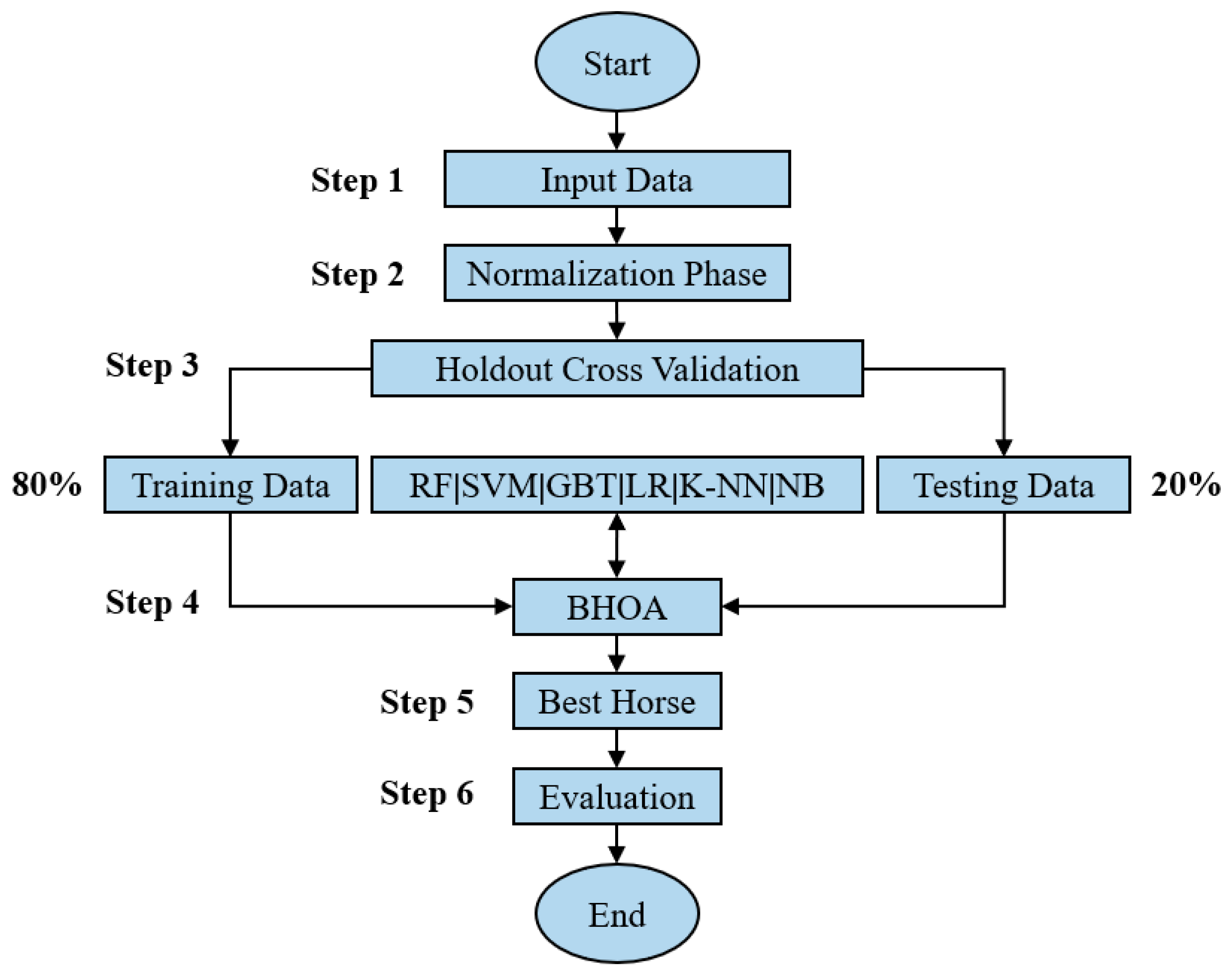
Figure 2 presents the high-level view of the BHOA machine learning methodology for feature selection.

The proposed methodology has the following steps:

• Step 1. The input data is represented by a dataset characterized by data samples with an equal number of features, which is a number greater than $1$, a label which is an integer value greater than or equal to $0$, and features described by real numerical values.
• Step 2. In the normalization phase, the values corresponding to the features are normalized to take values from $\left[0, 1\right]$, while the labels are not altered.
• Step 3. In the holdout cross-validation phase, the input data is split randomly into 80% training data and 20% testing data.
• Step 4. The BHOA algorithm is applied in feature selection. For each running of the algorithm, a different $Classifier$ from the possible classifiers RF, SVM, GBT, LR, K-NN, and NB, is selected. The objective function $OF$ is adapted to the following formula:

  $$OF\left(x\right)=\frac{1}{4}\times \frac{x_{selected features}}{x_{all features}}+\frac{3}{4}\times RMSE\left(Classifier, x\right),$$

  (7)

  where $x_{selected features}$ is the number of selected features which is equal to the number of $1^{\prime }$s of the position $x$, $x_{all features}$ is equal to $D$, which is the number of dimensions of the search space, and $RMSE\left(Classifier, x\right)$ is the Root Mean Squared Error (RMSE), computed using as parameters the testing data and the values predicted by the $Classifier$ when the features were selected according to $x_{selected features}$.
• Step 5. The best horse is the one for which the value of $OF\left(x\right)$ is minimal, as the objective of the optimization problem is to obtain the best prediction results using as few features as possible.
• Step 6. The $Classifier$ performance is evaluated using the standard classification metrics:

  $$accuracy=\frac{TP+TN}{TP+TN+FP+FN},$$

  (8)

  $$precision=\frac{TP}{TP+FP},$$

  (9)

  $$F1 score=\frac{2\times TP}{2\times TP+FP+FN},$$

  (10)

  where $TP$, $TN$, $FP$, and $FN$ are the true positives, true negatives, false positives, and false negatives for binary classification problems. The $recall$ metric was not considered because for multi-label classification problems the value of the $weighted recall$ is equal to the value of the $accuracy$. In particular, the values for $precision$ and $F1 score$ are computed as weighted values.

4. Results

The experiments were performed on a machine with the following characteristics: Intel(R) Core(TM) i7-7500 CPU @ 2.70 GHz processor, 8.00 GB installed RAM, 64-bit operating system, and x64-based processor.

For each dataset, a single experiment was run for each classifier from the possible classifiers RF, SVM, GBT, LR, K-NN, and NB, respectively. Each algorithm was trained using the training data and the classification metrics were computed using the testing data and the data predicted by the algorithm. No validation set was included in the experiments, as the methodology considered the simplest case of cross-validation, namely, holdout cross-validation, such that the set of all samples is represented by the union of the training data samples and the testing data samples.

Table 1. Classifier Configurations.

Classifier	Configuration
RF	10 estimators, 42 random state
SVM	0.00001 tolerance, 42 random state
GBT	10 estimators, 1.0 or 0.001 learning rate
LR	default parameters
K-NN	9 neighbors
NB	default or 100,000 var smoothing

presents the sklearn configurations of the classifiers used in experiments.

The configurations of the classifiers were selected after a series of in-house experiments with the objective of improving the running time of the classifiers compared to the cases where the default values of those parameters were used. In the case of K-NN, the value 9 was selected, bearing in mind that some studies suggest that an optimal value of K is the nearest integer to $\sqrt{n_{samples}}$, where $n_{samples}$ is the number of samples of the training data. The dataset with the minimum number of samples, namely, Breast Cancer Coimbra Data [37], had $n_{samples}$ = 93 for the training data; consequently a value of K equal to $\left[\sqrt{93}\right]=\left[9.643650\right]=9$ was used in the experiments. The value of this parameter led to good results for the other experimental datasets, therefore K = 9 was applied for all the experimental datasets. The value 100,000 for the parameter var smoothing for NB and the value 0.001 for the parameter learning rate for GBT were applied only to the Cervical Cancer (Risk Factors) Data Set [38]. For all other experimental datasets, the default value for the var smoothing parameter was considered for NB and a 1.0 learning rate value was considered for GBT.

4.1. Experimental Data Description

The datasets used in the experiments are presented next. All nine datasets were taken from the UCI machine learning repository, are representative for classification problems, and are from various research domains. The datasets were preprocessed for the proposed methodology as follows:

(1)

Smart Grids Data: The original data is the Electrical Grid Stability Simulated Data Dataset. The dataset was generated for a smart grid with one producer and three consumers, and the features describe the reaction time of the participants, the power consumed/produced, and the gamma coefficients of the price elasticity. The 13th feature, which represents the maximal real part corresponding to the characteristic equation root, is removed. The 14th feature is represented by the labels column. The values ‘stable’ and ‘unstable’ are converted into 1 and 0, respectively.

(2)

Raisin Data [39]: This dataset contains information from images of Besni and Kecimen raisin varieties that were grown in Turkey. The features describe the area, perimeter, major axis length, minor axis length, eccentricity, convex area, and extent. The labels column is represented by the ‘class’ column. The labels ‘Kecimen’ and ‘Besni’ were converted into 0 and 1, respectively.

(3)

Turkish Music Emotion Data [40]: The data are developed as a discrete model. The four classes of this data are ‘happy’, ‘sad’, ‘angry’, and ‘relaxed’. The dataset is prepared using non-verbal music and verbal music from various genres of Turkish music. The labels ‘happy’, ‘sad’, ‘angry’, and ‘relaxed’ are converted into 1, 2, 3, and 0, respectively.

(4)

Diabetes Risk Prediction Data [41]: The original data are from the Early Stage Diabetes Risk Prediction Dataset. The features contain information about the age of the monitored subjects and various conditions such as obesity, visual blurring, and delayed healing. The labels column is called ‘class’, and the two types of possible labels are ‘positive’ and ‘negative’. The categorical values are converted to numerical values as follows: ‘female’, ‘yes’, and ‘positive’ are converted to 1, while ‘male’, ‘no’, and ‘negative’ are converted to 0.

(5)

Rice Data [42]: The Rice (Cammeo and Osmancik) Data Set contains data about the Osmancik and Cammeo species of rice. For each grain of rice, seven morphological features were extracted, namely, the area, perimeter, major axis length, minor axis length, extent, convex area, and eccentricity. The ‘class’ column represents the labels. The values ‘Cammeo’ and ‘Osmancik’ were converted into 0 and 1, respectively.

(6)

Parkinson’s Disease Data [43]: The Parkinson’s Disease Classification Data Set was gathered from 108 patients with Parkinson’s Disease, as follows: 81 women and 107 men. The 64 healthy individuals are represented by 41 women and 23 men. The column ‘id’ was removed in the preprocessed data.

(7)

Cervical Cancer Data: The Cervical Cancer (Risk Factors) Data Set contains data which were collected at the Hospital Universitario de Caracas in Caracas, Venezuela. The data were collected from 858 patients, and describe demographic information, historical medical records, and habits. The missing values were replaced using the mean heuristic. The four target variables ‘Hinselmann’, ‘Schiller’, ‘cytology’, and ‘biopsy’ were converted into a single target variable equal to $2^3\times Hinselmann+2^2\times Schiller+2^1\times Cytology+2^0\times Biopsy$. This conversion led to the following set of labels: {0, 1, 2, 3, 4, 5, 6, 7, 8, 12, 13, 14, 15}. Then, the labels {12, 13, 14, 15} were converted into {9, 10, 11, 12}, such that the final labels were {0, 1, 2, 3, 4, 5, 6, 7, 8, 9, 10, 11, 12}.

(8)

Chronic Kidney Disease Data: These data can be used to predict chronic kidney disease, and the attributes contain information about various characteristics such as age, blood pressure, sugar, specific gravity, and red blood cell count. The values ‘abnormal’, ‘notpresent’, ‘no’, ‘poor’, and ‘notckd’ were converted to 0, while the categorical values ‘normal’, ‘present’, ‘yes’, ‘good’, and ‘ckd’ were converted to 1. The missing values were replaced using the mean heuristic.

(9)

Breast Cancer Coimbra Data: The data are characterized by nine features which describe quantitative data, such as age, Body Mass Index (BMI), and glucose level, and one ‘labels’ column. In the initial version of the data, the healthy controls were labeled with 1, while the patients were labeled with 2. In the processed data, the healthy controls and the patients were labeled with 0 and 1, respectively.

Table 2. Experimental Datasets Summary.

Experimental Dataset	Labels Number	Features Number	Training Data Samples Number	Testing Data Samples Number
Smart Grids Data	2	12	8000	2000
Raisin Data	2	7	720	180
Turkish Music Emotion Data	4	50	320	80
Diabetes Risk Prediction Data	2	16	416	104
Rice Data	2	6	3048	762
Parkinson’s Disease Data	2	753	605	151
Cervical Cancer Data	13	32	686	172
Chronic Kidney Disease Data	2	24	320	80
Breast Cancer Coimbra Data	2	9	93	23

summarizes the properties of the datasets after the preprocessing. For each dataset, the table presents the number of labels, the number of features, the number of samples of the training data, and the number of samples of the testing data.

4.2. BHOA Experimental Results

Table 3. BHOA Configuration Parameters.

Configuration Parameter	Value
$I$ (number of iterations)	50
$N$ (number of horses)	30
$M$ (horses reorganization frequency)	5
$DSP$ (dominant stallions percent)	10%
$HDR$ (horses distribution rate)	10%
$HMP$ (horse memory pool)	3
$SSP$ (single stallions percent)	10%

presents the configuration parameters of the BHOA used in experiments.

The value of $D$ is different for each dataset, and is equal to the number of features from Table 2. The objective function $OF$ is represented by Formula (7).

Table 4. BHOA Experimental Results Summary.

Dataset	Classifier	Accuracy	Precision	F1 Score	EvalGBest	(nf, RMSE)	Time (ms)
Smart Grids Data	RF	0.912	0.912548	0.910972	0.409985	(9, 0.296647)	998,676
	SVM	0.694	0.686913	0.666302	0.456546	(2, 0.553172)	361,459
	GBT	0.899	0.898627	0.898736	0.425853	(9, 0.317804)	1,411,226
	LR	0.6935	0.685425	0.667392	0.456884	(2, 0.553624)	127,434
	K-NN	0.897	0.897719	0.895522	0.407368	(8, 0.320936)	1,509,808
	NB	0.7005	0.697274	0.670953	0.452116	(2, 0.547265)	19,477
Raisin Data	RF	0.85	0.858348	0.849698	0.361902	(2, 0.387298)	109,878
	SVM	0.872222	0.880895	0.871965	0.339523	(2, 0.357460)	17,181
	GBT	0.866666	0.870097	0.866666	0.345289	(2, 0.365148)	89,852
	LR	0.855555	0.865277	0.855180	0.356472	(2, 0.380058)	26,454
	K-NN	0.85	0.860997	0.849513	0.361902	(2, 0.387298)	38,053
	NB	0.85	0.864039	0.849289	0.361902	(2, 0.387298)	5984
Turkish Music Emotion Data	RF	0.9	0.905083	0.900721	0.545	(34, 0.5)	125,597
	SVM	0.925	0.923872	0.922807	0.485473	(39, 0.387298)	169,451
	GBT	0.775	0.811160	0.786773	0.589279	(26, 0.612372)	797,135
	LR	0.925	0.929673	0.923135	0.530756	(35, 0.474341)	308,861
	K-NN	0.825	0.832499	0.823849	0.685330	(31, 0.707106)	40,878
	NB	0.85	0.857903	0.851368	0.514260	(26, 0.512347)	11,822
Diabetes Risk Prediction Data	RF	0.990384	0.990619	0.990406	0.198543	(8, 0.098058)	82,800
	SVM	0.942307	0.942307	0.942307	0.305144	(8, 0.240192)	15,158
	GBT	1.0	1.0	1.0	0.1875	(12, 0.0)	45,600
	LR	0.932692	0.933172	0.932842	0.319577	(8, 0.259437)	26,535
	K-NN	0.932692	0.935100	0.933101	0.288327	(6, 0.259437)	29,988
	NB	0.951923	0.954133	0.952215	0.305073	(9, 0.219264)	6495
Rice Data	RF	0.913385	0.913333	0.913302	0.304060	(2, 0.294302)	240,551
	SVM	0.923884	0.924280	0.923666	0.290251	(2, 0.275890)	36,531
	GBT	0.914698	0.914767	0.914538	0.302381	(2, 0.292064)	286,505
	LR	0.922572	0.922770	0.922397	0.292027	(2, 0.278258)	72,552
	K-NN	0.922572	0.922890	0.922366	0.292027	(2, 0.278258)	145,352
	NB	0.922572	0.922553	0.922484	0.292027	(2, 0.278258)	8526
Parkinson’s Disease Data	RF	0.847682	0.852720	0.849814	0.333878	(124, 0.390279)	759,970
	SVM	0.860927	0.856619	0.848757	0.300941	(64, 0.372924)	2,663,289
	GBT	0.860927	0.862374	0.861605	0.335037	(187, 0.363937)	4,859,351
	LR	0.860927	0.859675	0.846185	0.317210	(113, 0.372924)	845,271
	K-NN	0.860927	0.859675	0.846185	0.318538	(117, 0.372924)	1,279,114
	NB	0.821192	0.823018	0.822064	0.355323	(115, 0.422856)	519,532
Cervical Cancer Data	RF	0.889534	0.908949	0.847967	1.574075	(14, 1.952934)	140,590
	SVM	0.889534	0.901737	0.837531	1.732502	(4, 2.268336)	197,975
	GBT	0.889534	0.901737	0.837531	1.732502	(4, 2.268336)	969,271
	LR	0.889534	0.901737	0.837531	1.732502	(4, 2.268336)	214,834
	K-NN	0.889534	0.901737	0.837531	1.732502	(4, 2.268336)	70,139
	NB	0.889534	0.901737	0.837531	1.732502	(4, 2.268336)	15,678
Chronic Kidney Disease Data	RF	1.0	1.0	1.0	0.09375	(9, 0.0)	91,848
	SVM	1.0	1.0	1.0	0.083333	(8, 0.0)	13,385
	GBT	1.0	1.0	1.0	0.083333	(8, 0.0)	60,803
	LR	1.0	1.0	1.0	0.104166	(10, 0.0)	30,407
	K-NN	1.0	1.0	1.0	0.09375	(9, 0.0)	26,898
	NB	1.0	1.0	1.0	0.145833	(14, 0.0)	6673
Breast Cancer Coimbra Data	RF	0.913043	0.926421	0.912714	0.304496	(3, 0.294883)	84,961
	SVM	0.826086	0.826086	0.826086	0.423882	(4, 0.417028)	7934
	GBT	0.913043	0.913043	0.913043	0.360051	(5, 0.294883)	38,080
	LR	0.739130	0.826086	0.716304	0.438620	(2, 0.510753)	17,734
	K-NN	0.826086	0.869565	0.819185	0.368327	(2, 0.417028)	11,024
	NB	0.782608	0.850543	0.774133	0.460800	(4, 0.466252)	5248

presents the BHOA experimental results. The columns are: (1) Dataset—the preprocessed data used in experiments, (2) Classifier—one of the classifiers from the possible set of classifiers {RF, SVM, GBT, LR, K-NN, NB}, (3) Accuracy—the accuracy for testing data, (4) Precision—the precision for testing data, (5) F1 score—the F1 score for testing data, (6) EvalGBest—the evaluated value of the global best individual after the running of all iterations, (7) (nf, RMSE)—the number of selected features and the RMSE computed using the testing data and the applied classifier, and (8) Time (ms)—the running time of the algorithm for $I$ iterations.

As can be seen in the table, the classifier that returned the best accuracy results was SVM, as it returned the best accuracy results for six out of the nine datasets used in the experiments. Another observation is that all classifiers returned the best accuracy result for the Chronic Kidney Disease Data.

The classifier which returned the best $EvalGBest$ value in most cases was SVM as it returned the best value for five datasets.

Table 5. BHOA GBest Values Results Summary.

Dataset	Classifier	GBest Value
Smart Grids Data	RF	[111110001111]
	SVM	[100000000010]
	GBT	[111100101111]
	LR	[100000000010]
	K-NN	[111100001111]
	NB	[100000000010]
Raisin Data	RF	[1001000]
	SVM	[10001]
	GBT	[1000001]
	LR	[110]
	K-NN	[10001]
	NB	[100001]
Turkish Music Emotion Data	RF	[01011111111101111111110110101110110110101000101010]
	SVM	[11111111101110101111011111111011101110111001100111]
	GBT	[01111110111010011010101101010101010101100010010000]
	LR	[11110010110111010111111011111101000110111011110110]
	K-NN	[11111101011111000001111011011101111101011000010010]
	NB	[01111100111101110001110000010011111110000000010011]
Diabetes Risk Prediction Data	RF	[1101100000111100]
	SVM	[0101101110110000]
	GBT	[1101011101110111]
	LR	[1101101110100000]
	K-NN	[1101101000010000]
	NB	[1101101010110010]
Rice Data	RF	[100001]
	SVM	[001010]
	GBT	[110000]
	LR	[110000]
	K-NN	[001010]
	NB	[110000]
Parkinson’s Disease Data	RF	[000011000000000000001100000000001000000000000001000001000001000000101010000000000110000000100010000010000100001000011011000000000000000000010000000001000000000000000000100000001000000010010010011000000011010000100000000000000100100000000010000100001000000000100000000100000001011100000001000000001000001100000000000000000101000001000000000110000000111000100011100000000000010000100000000000001101000001110000000000000000000100001010000000000000000000000000100100100000100010000000000000000000000000100000110010100010000000010000000010000100000000000101000000000010000000000001000000100001000100000000010000010001000000000000001000101000000000011000000011001000010010000000010110000110001000000000001000000000000100100000000010010000000100000010110011000]
	SVM	[000010000000000000000000100000010000000000000100010000000000000000000100000000000000000000000000010000010000000000001000000000010000000000010000000000000000000000000000010001001000000000010000000000001000100000000000000000000000000000000011000000000000000000000001001000000011010000000000000000000000000000000000000000000000000100000000000000000000000000000001000000100000000001000000001000000000000000000100001000100000000000000010000001001000010010000001001000001000000000000000000011000000000000000001000000000001000000000000000001000000000000000000000000000000001000000000000000000010000000000000001000000010011000100000000000000000000000000000010000000000000000000000000010001000001000000000000000000011000000100100000000100000000001010000000000100]
	GBT	[100001010010110000110000010001010000000010101000100001101001010000000000011010100100000010000000010100000000100110001100101001100010100001010010000001010000010110011000101000000010000001000000000000110010010000000000000000000000001010001000000110100101001001100001000001010001010001001110001000000000000100000100001000000000010000100000000010100011000100010000100000000000101000010000000011001100000001110001101000010000000001000010010000100100100100110100000000011000000000001111001000000110000010101011000100110001000000110110000010100001000000000100000010111000000001001000010100000000000100001001111100000000011000100011000100001101001000000000000001000101000001000000000010000110001010000110000000000001100000000000000000000010000001000111010110001]
	LR	[000010000001000000000000100000110000000001000101010001000100000000101100000010000100000000000000010000011000000000001000000000010001000001010010000000100000000000000001010001001000000000010001000001001000100000000000000000000100000000000011000000100000000000000001101000000011110000000010100000000000001000010001000000000100000100000000010000000000001000001001000001100000000001000000001000100000000000000100001000100000100000000010000001001000010010010001001000001000000000000000000011001000000001000001100000010001000000000000000001000110000000001100000000100000001000000000001000000011000100000000001000000000011000100001000000000000000000001000010000001000000000000000001010001000001000000000000000000010000000100100000000100000000001010000000000100]
	K-NN	[000010000100100100000001000100001001000000000000000000011000000000000000011000000010000100000000000010001000001000000001000001010000101001101000000001001000001001000000100000110000100000000100110001000100000000000010000100100000001000000000000000100000000100001000001010100000010001000000000000010000110010000000010001000001000000000010000000000000000000100001000001000000000010000101000000010000000000100000100000001100000000000000001000100000001011000000000000101101000000010010000000000000000001000001000000100000101010000000000000000001000000000000001100000000010000000000000001000010010010000000000000000001100000001000001000001000110001000100000001000000010001000100000000000100001101000000000000110000001000000000000000100001000000000000000000001]
	NB	[000000001000100001010000000101000000100000010001000000000000001100100000000100000000010100000100000001000000010000100000010000000000000000001000000010000000000000000000000000000010001011000000110000000010100000110110000000000100000000000000000000000000000000000100100000010000000101000000000010000010100010000110100000000000010000000000011000010010010010100000010000101000001010000000001000010000000000101000100000100000100001100010001000001000000000000000100000000011000000010000010000000000000100000000000101000000100000100000000000000000000000110000000010000101010000000000000110000000000000000000000000010100100101000000000000100110000001110001000000001000000000000001000000000001000000101000000000000000000000101010100000000010100000001000001000000]
Cervical Cancer Data	RF	[11110101010001010101100100100000]
	SVM	[00010000000100010000000000000001]
	GBT	[00010000000100010000000000000001]
	LR	[00010000000100010000000000000001]
	K-NN	[00100000000000000001001000000100]
	NB	[00010000000100010000000000000001]
Chronic Kidney Disease Data	RF	[000101110000101100101000]
	SVM	[111011010000001000001000]
	GBT	[101010000010110100000010]
	LR	[111011010100001001001000]
	K-NN	[000110001000011011010100]
	NB	[111101001011001101111000]
Breast Cancer Coimbra Data	RF	[101001000]
	SVM	[101010010]
	GBT	[101001011]
	LR	[001100000]
	K-NN	[100100000]
	NB	[111000010]

presents the summary of the BHOA $GBest$ values. The selected features are marked with 1, while the features which are not selected are marked with 0.

As can be seen in the table, the features selected by the BHOA differ significantly for each classifier, even in cases when the same values for accuracy, precision, and F1 score were obtained, as in the case of Chronic Kidney Disease Data, which can be seen in Table 4.

5. Discussion

This section compares the BHOA to binary versions of the GWO, PSO, and CSA as follows:

(1)

Binary Grey Wolf Optimizer (BGWO);

(2)

Binary Particle Swarm Optimization (BPSO);

(3)

Binary Crow Search Algorithm (BCSA).

Table 6. BGWO Configuration Parameters.

Configuration Parameter	Value
$I$ (number of iterations)	50
$N$ (number of wolves)	30

,

Table 7. BPSO Configuration Parameters.

Configuration Parameter	Value
$I$ (number of iterations)	50
$N$ (number of particles)	30
$w$ (initial inertia value)	0.901
$c_1$ (cognitive component constant)	2
$c_2$ (social component constant)	2

and

Table 8. BCSA Configuration Parameters.

Configuration Parameter	Value
$I$ (number of iterations)	50
$N$ (number of crows)	30
$fl$ (flight length)	0.9
$AP$ (awareness probability)	0.5

present the configuration parameters for the BGWO, BPSO, and BCSA which were used in experiments.

Table 9. BGWO Experimental Results Summary.

Dataset	Classifier	Accuracy	Precision	F1 score	EvalGBest	(nf, RMSE)	Time (ms)
Smart Grids Data	RF	0.912	0.912548	0.910972	0.409985	(9, 0.296647)	25,1259
	SVM	0.748	0.743291	0.739087	0.459830	(4, 0.501996)	60,674
	GBT	0.899	0.898627	0.898736	0.405020	(8, 0.317804)	332,609
	LR	0.7495	0.744781	0.741097	0.458708	(4, 0.500499)	21,082
	K-NN	0.897	0.897719	0.895522	0.407368	(8, 0.320936)	326,848
	NB	0.7315	0.728542	0.714810	0.451127	(3, 0.518169)	4087
Raisin Data	RF	0.85	0.858348	0.849698	0.361902	(2, 0.387298)	25,023
	SVM	0.861111	0.869622	0.860832	0.350937	(2, 0.372677)	3343
	GBT	0.866666	0.870097	0.866666	0.345289	(2, 0.365148)	16,658
	LR	0.855555	0.858942	0.855555	0.356472	(2, 0.380058)	6225
	K-NN	0.872222	0.878514	0.872092	0.339523	(2, 0.357460)	8892
	NB	0.844444	0.859980	0.843577	0.367232	(2, 0.394405)	1479
Turkish Music Emotion Data	RF	0.8875	0.889423	0.886550	0.515756	(32, 0.474341)	35,934
	SVM	0.9375	0.940368	0.937143	0.418107	(28, 0.370809)	31,204
	GBT	0.825	0.834703	0.828157	0.579262	(32, 0.559016)	190,036
	LR	0.9125	0.913035	0.910288	0.437334	(27, 0.403112)	68,773
	K-NN	0.85	0.861757	0.848489	0.544260	(32, 0.512347)	11,434
	NB	0.8625	0.861807	0.859248	0.52	(29, 0.5)	3132
Diabetes Risk Prediction Data	RF	1.0	1.0	1.0	0.1875	(12, 0.0)	21,041
	SVM	0.932692	0.935100	0.933101	0.288327	(6, 0.259437)	3359
	GBT	0.990384	0.990619	0.990406	0.229793	(10, 0.098058)	11,020
	LR	0.932692	0.942716	0.933453	0.272702	(5, 0.259437)	5473
	K-NN	0.942307	0.946037	0.942750	0.273894	(6, 0.240192)	6570
	NB	0.894230	0.894874	0.894467	0.273823	(5, 0.260931)	1477
Rice Data	RF	0.910761	0.910761	0.910761	0.307379	(2, 0.298728)	47,690
	SVM	0.923884	0.924280	0.923666	0.290251	(2, 0.275890)	7404
	GBT	0.916010	0.916127	0.915837	0.300690	(2, 0.289809)	51,724
	LR	0.919947	0.920249	0.919734	0.295534	(2, 0.282935)	10,566
	K-NN	0.916010	0.916127	0.915837	0.300690	(2, 0.289809)	33,522
	NB	0.921259	0.921400	0.921097	0.293788	(2, 0.280606)	2140
Parkinson’s Disease Data	RF	0.920529	0.918877	0.918795	0.355813	(462, 0.269903)	133,329
	SVM	0.947019	0.950437	0.944484	0.301116	(387, 0.230174)	637,241
	GBT	0.900662	0.897880	0.897889	0.358514	(392, 0.304491)	965,475
	LR	0.907284	0.906097	0.902848	0.347226	(358, 0.304491)	183,896
	K-NN	0.920529	0.920877	0.916727	0.347218	(409, 0.281904)	235,658
	NB	0.834437	0.829944	0.831787	0.430336	(378, 0.406451)	22,674
Cervical Cancer Data	RF	0.889534	0.909969	0.845334	1.563974	(11, 1.970715)	32,820
	SVM	0.889534	0.901737	0.837531	1.724689	(3, 2.268336)	39,130
	GBT	0.889534	0.901737	0.837531	1.724689	(3, 2.268336)	180,010
	LR	0.889534	0.901737	0.837531	1.724689	(3, 2.268336)	32,845
	K-NN	0.889534	0.901737	0.837531	1.724689	(3, 2.268336)	10,959
	NB	0.889534	0.901737	0.837531	1.724689	(3, 2.268336)	3971
Chronic Kidney Disease Data	RF	1.0	1.0	1.0	0.0625	(6, 0.0)	20,445
	SVM	1.0	1.0	1.0	0.0625	(6, 0.0)	2410
	GBT	1.0	1.0	1.0	0.083333	(8, 0.0)	13,438
	LR	1.0	1.0	1.0	0.052083	(5, 0.0)	10,193
	K-NN	1.0	1.0	1.0	0.052083	(5, 0.0)	5905
	NB	1.0	1.0	1.0	0.09375	(9, 0.0)	1539
Breast Cancer Coimbra Data	RF	0.826086	0.835058	0.824080	0.396104	(3, 0.417028)	20,000
	SVM	0.782608	0.801086	0.777523	0.423882	(3, 0.454065)	1665
	GBT	0.869565	0.871906	0.869068	0.409757	(5, 0.361157)	9323
	LR	0.826086	0.869565	0.819185	0.396104	(3, 0.417028)	4061
	K-NN	0.869565	0.871906	0.869068	0.409757	(5, 0.361157)	2635
	NB	0.782608	0.783946	0.781780	0.433022	(3, 0.466252)	1276

,

Table 10. BPSO Experimental Results Summary.

Dataset	Classifier	Accuracy	Precision	F1 score	EvalGBest	(nf, RMSE)	Time (ms)
Smart Grids Data	RF	0.912	0.912548	0.910972	0.409985	(9, 0.296647)	248,483
	SVM	0.7575	0.754617	0.747401	0.452665	(4, 0.492442)	89,348
	GBT	0.899	0.898627	0.898736	0.405020	(8, 0.317804)	329,124
	LR	0.758	0.754943	0.748261	0.452284	(4, 0.491934)	31,514
	K-NN	0.897	0.897719	0.895522	0.407368	(8, 0.320936)	316,462
	NB	0.7755	0.778501	0.763177	0.438694	(4, 0.473814)	4771
Raisin Data	RF	0.822222	0.837050	0.821231	0.361902	(3, 0.339679)	27,490
	SVM	0.85	0.856079	0.849847	0.339523	(3, 0.309841)	4111
	GBT	0.866666	0.870097	0.866666	0.345289	(2, 0.365148)	23,406
	LR	0.855555	0.862789	0.855341	0.356472	(2, 0.380058)	6817
	K-NN	0.872222	0.878514	0.872092	0.339523	(2, 0.357460)	9630
	NB	0.855555	0.860681	0.855466	0.356472	(2, 0.380058)	1610
Turkish Music Emotion Data	RF	0.8125	0.828781	0.817075	0.559279	(20, 0.612372)	37,558
	SVM	0.875	0.881037	0.876875	0.518303	(25, 0.524404)	35,201
	GBT	0.8125	0.819272	0.813236	0.609341	(27, 0.632455)	156,980
	LR	0.8375	0.841059	0.835601	0.504262	(17, 0.559016)	53,802
	K-NN	0.7625	0.784397	0.763781	0.668072	(7, 0.844097)	8584
	NB	0.8625	0.862634	0.858907	0.525732	(36, 0.460977)	2265
Diabetes Risk Prediction Data	RF	1.0	1.0	1.0	0.125	(8, 0.0)	20,847
	SVM	0.884615	0.889044	0.885501	0.286012	(2, 0.339683)	3908
	GBT	0.990384	0.990532	0.990361	0.214168	(9, 0.098058)	11,035
	LR	0.884615	0.889044	0.885501	0.286012	(2, 0.339683)	6369
	K-NN	0.961538	0.962601	0.961702	0.256462	(7, 0.196116)	7427
	NB	0.884615	0.889044	0.885501	0.286012	(2, 0.339683)	1488
Rice Data	RF	0.913385	0.913385	0.913385	0.304060	(2, 0.294302)	60,536
	SVM	0.923884	0.924280	0.923666	0.290251	(2, 0.275890)	9229
	GBT	0.916010	0.916127	0.915837	0.300690	(2, 0.289809)	68,857
	LR	0.919947	0.920249	0.919734	0.295534	(2, 0.282935)	18,202
	K-NN	0.922572	0.922890	0.922366	0.292027	(2, 0.278258)	36,409
	NB	0.921259	0.921400	0.921097	0.293788	(2, 0.280606)	2196
Parkinson’s Disease Data	RF	0.900662	0.898439	0.899072	0.295813	(179, 0.315178)	107,492
	SVM	0.920529	0.920877	0.916727	0.270857	(179, 0.281904)	420,036
	GBT	0.907284	0.904998	0.905260	0.263561	(106, 0.304491)	743,155
	LR	0.900662	0.902048	0.893650	0.286184	(150, 0.315178)	130,233
	K-NN	0.894039	0.890771	0.890408	0.298585	(164, 0.325515)	151,805
	NB	0.847682	0.846218	0.846905	0.318605	(78, 0.390279)	17,699
Cervical Cancer Data	RF	0.889534	0.894736	0.840116	1.662037	(7, 2.143133)	49,912
	SVM	0.889534	0.901737	0.837531	1.716877	(2, 2.268336)	45,406
	GBT	0.889534	0.901737	0.837531	1.716877	(2, 2.268336)	220,140
	LR	0.889534	0.901737	0.837531	1.716877	(2, 2.268336)	40,927
	K-NN	0.889534	0.901737	0.837531	1.716877	(2, 2.268336)	16,559
	NB	0.889534	0.901737	0.837531	1.716877	(2, 2.268336)	3805
Chronic Kidney Disease Data	RF	1.0	1.0	1.0	0.052083	(5, 0.0)	20,926
	SVM	1.0	1.0	1.0	0.09375	(9, 0.0)	2718
	GBT	1.0	1.0	1.0	0.052083	(5, 0.0)	14,586
	LR	1.0	1.0	1.0	0.083333	(8, 0.0)	7743
	K-NN	1.0	1.0	1.0	0.083333	(8, 0.0)	6437
	NB	0.9875	0.987735	0.987445	0.167185	(8, 0.111803)	1539
Breast Cancer Coimbra Data	RF	0.913043	0.926421	0.912714	0.332274	(4, 0.294883)	20,374
	SVM	0.652173	0.652173	0.652173	0.423882	(6, 0.342954)	1862
	GBT	0.608695	0.611956	0.599542	0.360051	(6, 0.257846)	9458
	LR	0.826086	0.869565	0.819185	0.396104	(3, 0.417028)	7177
	K-NN	0.913043	0.913043	0.913043	0.332274	(4, 0.294883)	2644
	NB	0.782608	0.783946	0.781780	0.433022	(3, 0.466252)	1433

and

Table 11. BCSA Experimental Results Summary.

Dataset	Classifier	Accuracy	Precision	F1 score	EvalGBest	(nf, RMSE)	Time (ms)
Smart Grids Data	RF	0.891	0.891429	0.889478	0.414280	(8, 0.330151)	226,327
	SVM	0.713	0.713693	0.685312	0.443459	(2, 0.535723)	72,052
	GBT	0.899	0.898627	0.898736	0.405020	(8, 0.317804)	258,876
	LR	0.713	0.712269	0.686781	0.443459	(2, 0.535723)	24,238
	K-NN	0.897	0.897719	0.895522	0.407368	(8, 0.320936)	188,415
	NB	0.7085	0.711154	0.676842	0.446597	(2, 0.539907)	4146
Raisin Data	RF	0.855555	0.868158	0.854983	0.356472	(2, 0.380058)	26,458
	SVM	0.872222	0.880895	0.871965	0.339523	(2, 0.357460)	3743
	GBT	0.866666	0.870097	0.866666	0.345289	(2, 0.365148)	19,151
	LR	0.855555	0.862789	0.855341	0.356472	(2, 0.380058)	6513
	K-NN	0.872222	0.878514	0.872092	0.339523	(2, 0.357460)	9179
	NB	0.855555	0.860681	0.855466	0.356472	(2, 0.380058)	1441
Turkish Music Emotion Data	RF	0.8625	0.872173	0.862413	0.532142	(26, 0.536190)	30,483
	SVM	0.925	0.926199	0.922436	0.454759	(26, 0.433012)	35,100
	GBT	0.8	0.816792	0.804053	0.568705	(25, 0.591607)	140,459
	LR	0.8875	0.891218	0.886330	0.530791	(24, 0.547722)	47,209
	K-NN	0.7625	0.790690	0.767970	0.630330	(20, 0.707106)	8163
	NB	0.8125	0.821741	0.814935	0.535791	(25, 0.547722)	1939
Diabetes Risk Prediction Data	RF	0.990384	0.990532	0.990361	0.198543	(8, 0.098058)	20,801
	SVM	0.903846	0.916895	0.905011	0.295065	(4, 0.310086)	3723
	GBT	0.990384	0.990619	0.990406	0.198543	(8, 0.098058)	10,362
	LR	0.903846	0.916895	0.905011	0.295065	(4, 0.310086)	5936
	K-NN	0.980769	0.981684	0.980851	0.244631	(9, 0.138675)	6770
	NB	0.942307	0.943518	0.942553	0.289519	(7, 0.240192)	1393
Rice Data	RF	0.913385	0.913333	0.913302	0.304060	(2, 0.294302)	54,663
	SVM	0.923884	0.924280	0.923666	0.290251	(2, 0.275890)	8067
	GBT	0.912073	0.912460	0.911803	0.300690	(2, 0.289809)	57,991
	LR	0.922572	0.922770	0.922397	0.292027	(2, 0.278258)	14,810
	K-NN	0.922572	0.922890	0.922366	0.292027	(2, 0.278258)	34,673
	NB	0.922572	0.922553	0.922484	0.292027	(2, 0.278258)	2132
Parkinson’s Disease Data	RF	0.913907	0.913134	0.913468	0.337923	(355, 0.293415)	118,080
	SVM	0.933774	0.932756	0.932329	0.319168	(380, 0.257342)	499,655
	GBT	0.907284	0.905061	0.904107	0.339922	(336, 0.304491)	864,187
	LR	0.907284	0.908293	0.901474	0.357186	(388, 0.304491)	134,454
	K-NN	0.894039	0.892925	0.887398	0.369634	(378, 0.325515)	149,951
	NB	0.821192	0.826924	0.823694	0.435004	(355, 0.422856)	13,405
Cervical Cancer Data	RF	0.843023	0.841024	0.824169	1.662473	(11, 2.102047)	29,424
	SVM	0.889534	0.901737	0.837531	1.755939	(7, 2.268336)	47,669
	GBT	0.889534	0.901737	0.837531	1.755939	(7, 2.268336)	207,039
	LR	0.889534	0.901737	0.837531	1.755939	(7, 2.268336)	38,510
	K-NN	0.889534	0.901737	0.837531	1.755939	(7, 2.268336)	14,752
	NB	0.889534	0.901737	0.837531	1.755939	(7, 2.268336)	3392
Chronic Kidney Disease Data	RF	1.0	1.0	1.0	0.072916	(7, 0.0)	20,432
	SVM	1.0	1.0	1.0	0.0625	(6, 0.0)	2326
	GBT	1.0	1.0	1.0	0.072916	(7, 0.0)	12,809
	LR	1.0	1.0	1.0	0.0625	(6, 0.0)	7381
	K-NN	1.0	1.0	1.0	0.0625	(6, 0.0)	5904
	NB	1.0	1.0	1.0	0.09375	(9, 0.0)	1415
Breast Cancer Coimbra Data	RF	0.913043	0.926421	0.912714	0.304496	(3, 0.294883)	21,385
	SVM	0.826086	0.826086	0.826086	0.423882	(4, 0.417028)	1723
	GBT	0.913043	0.913043	0.913043	0.304496	(3, 0.294883)	8984
	LR	0.826086	0.869565	0.819185	0.396104	(3, 0.417028)	4358
	K-NN	0.913043	0.913043	0.913043	0.332274	(4, 0.294883)	2646
	NB	0.782608	0.783946	0.781780	0.433022	(3, 0.466252)	1240

present the BGWO, BPSO, and BCSA experimental results, respectively.

In the case of the BGWO, the classifier which led to the best accuracy results for most of the datasets was SVM, as it returned the best accuracy for five out of the nine datasets. The classifiers which returned the best $EvalGBest$ were SVM and RF, because each one returned the best value for three out of the nine datasets.

The experimental results for the BPSO show that the algorithms which returned the best accuracy for most of the datasets (five out of nine), were RF and SVM. On the other hand, RF returned the best $EvalGBest$ value for four out of the nine datasets.

Finally, in the case of the BCSA, the SVM classifier returned the best accuracy for six out of the nine datasets, and the best $EvalGBest$ value for five out of the nine datasets as well.

Next,

Table 12. BGWO GBest Values Results Summary.

Dataset	Classifier	GBest Value
Smart Grids Data	RF	[111110001111]
	SVM	[101100000100]
	GBT	[111100001111]
	LR	[101100000100]
	K-NN	[111100001111]
	NB	[100100000100]
Raisin Data	RF	[1001000]
	SVM	[0000110]
	GBT	[1000001]
	LR	[0011000]
	K-NN	[1000100]
	NB	[0100010]
Turkish Music Emotion Data	RF	[01111111111100110111101100000111010001111010011011]
	SVM	[01110001101110001011000101011001110101110010011111]
	GBT	[11100110101110110111011001010001100011111101111011]
	LR	[11011111001111010111001101010001000100011100010110]
	K-NN	[10010111110111101111011101100110101111010000111010]
	NB	[11011110010010111010011101010111100000011001110111]
Diabetes Risk Prediction Data	RF	[1001111111011011]
	SVM	[0101101000110000]
	GBT	[0001101011111110]
	LR	[0101101000001000]
	K-NN	[0101001100110000]
	NB	[0011100000100100]
Rice Data	RF	[011000]
	SVM	[001010]
	GBT	[011000]
	LR	[011000]
	K-NN	[010001]
	NB	[011000]
Parkinson’s Disease Data	RF	[111011110111000110110001010100101100100111101010010110111111011101100111011011110100111001101101001101101011111000101001001111110100100011010011000111010010111001111010100010100100100110010010010101100101000111111000110110110111111111110010111101001011111101011110100011010100001001100011111100011010110011101111011101111101001111110101110111111111111111011110001101101101011101001110110000010111010001000111110111001111011001010100011100101010011111111100010101010100010010101010100110111001010110111110100110010111111111010011111110111101111111111100011110100001011001111110110010111011011111100111111110100011001010011011111011111011101101101111101011111001101100100101010011011111111111100001010111110011101101100001101100101111011111001001101101011]
	SVM	[010011110011111001100010110100101001100100011101010000111101010101111101111111111100000100101100001011100011011010101110111010001101111111101110100010111001011110101111000101110000110010000000000101010011100111110110110110010110010101100111100011011101101100011101111000101010110101101011100110011100000111000000100110100101011001110010001011011101101101001011010100111101101100001001110001001111100111101110100011111100101011110100001001011100000111100000110011110111110010101010000000001111110101001011010011010000011100110100000000010001010110001001111101000000010011010001001010010010111001110010011001001001101100110000001000001011000100001111010101111011110010011011110111011100101110101011110011110000010000001111010010011100101111001010111100100]
	GBT	[010000110110110101001000000010100101101000001111101101010001100001011101111011111101001000110111000100110010111100111110011011100000110100100100101110000010010100010101110101010101101001101010101011111101101000011100001000111110101000101001011101110011001001110100011111110001110100111011010110010101110011000011111011011011111100010110001000111001101101010011011001110000111110110011100101000001001111100000101100001011000100101100101011111001011011111111001100001011111110011010111110010100001000011110011110111011111111100011101000011000000010101010001110110100011110011101100010101000111011000110011011001001111010101110100110100111100001001100101001101011101010111100010010111110001110000100010000111000110010000111010101111111100110001010000010110]
	LR	[000101010111110010000111111011110010111110001011000000010110011001011111110110100111010100001100001101001111100100101000011100101100110011001111000001011011010000010001000000010100101011100000010001110111101001001100010000011110111011100011010111100101100100110100111011010011011111111110000110111010111111110010111011000011111001110010100000001101100101001110100010001110101010111000100011011001101000001010100011000111001010101000011010101000011100100100100101001110110001101001001111000011110011011000010100111010111000110000101011010001011010000001000101000100001010001011111011101100111111010000110100010110000010110011110101000010100011011100100000000001101011001010110100100101110011100100101000000101010001001000000111101000111000100100010100111]
	K-NN	[101000100101010010111001011111110101111011001101011010111111000001011010111100100001011110101110101100011110101110001011011101010110110111011001110011010110011010010100110001010110010111010000111100111110101001111001010010011010011011111011010101110010001101010100010101011011000011001010101011001001011110110010101001000001011001011100101000011111010010000010111001011001011001000000001010000100011011111010010000011010010011111000101011010111111100001101111010010111111111010101001001010100111011011111110110011111100011010111111011110011001101111111111100011010011100100011110111011110101011000011011001110010110000001000101110111011011100011100001010011111101010011110110011000101110011101100000101110000000001111101001101100000110010001110010111111]
	NB	[101110100011001010000000010001110000100100000111010111010011001011101100001000101001001110000111001111110110110100110010111000100010101110111100010100011001011000110100101010010101101101111110101110100110001001100100111010101011011001110101011111110010010001100100110100000000011110001000111101011001001111010001101000111001011101110001100100000111111011010100101011001111010100010001010101111000011001101000001011010010100000101110011111110111010101100101101111100111110011100111100000101001011000100110110111001001111010110100111100011111011111001111011100011100101101010001010111011101001001100101010010110100100001111000101000111110001000101100101010110010001001000110110100100101111100010000001001101101010010011011010101010000010100000110101101101]
Cervical Cancer Data	RF	[00110010010000100010001110010010]
	SVM	[00100000000010000001000000000000]
	GBT	[00100000000010000001000000000000]
	LR	[00100000000010000001000000000000]
	K-NN	[00100000000010000001000000000000]
	NB	[00100000000010000001000000000000]
Chronic Kidney Disease Data	RF	[001100000010000001010100]
	SVM	[001000000100101100010000]
	GBT	[110100000110100001000001]
	LR	[001000000000001110010000]
	K-NN	[001000000100001100010000]
	NB	[000101011001000101110000]
Breast Cancer Coimbra Data	RF	[001001010]
	SVM	[101100000]
	GBT	[111010010]
	LR	[001010010]
	K-NN	[101110010]
	NB	[110000010]

,

Table 13. BPSO GBest Values Results Summary.

Dataset	Classifier	GBest Value
Smart Grids Data	RF	[111110001111]
	SVM	[111000000001]
	GBT	[111100001111]
	LR	[111000000001]
	K-NN	[111100001111]
	NB	[111000000001]
Raisin Data	RF	[1101000]
	SVM	[1101000]
	GBT	[1000001]
	LR	[0100100]
	K-NN	[1000100]
	NB	[0011000]
Turkish Music Emotion Data	RF	[10100011101101001001000100000100010001010100110101]
	SVM	[11111011010100011010001100010001101100010011011010]
	GBT	[01001100111011011011000101111110001111000100100110]
	LR	[01110010000000001001001000110001100110011000110000]
	K-NN	[00001010000000000000100001010001000000000000010000]
	NB	[01100111011011010110011111111111111100111010110111]
Diabetes Risk Prediction Data	RF	[1101000000111110]
	SVM	[0101000000000000]
	GBT	[1101001111100010]
	LR	[0101000000000000]
	K-NN	[0001001100101101]
	NB	[0101000000000000]
Rice Data	RF	[100100]
	SVM	[001010]
	GBT	[011000]
	LR	[011000]
	K-NN	[001010]
	NB	[011000]
Parkinson’s Disease Data	RF	[000011100000001011000001001000000000000000010010001000101010000000000010001001001001000000000100000000110100000001100001000110001000001100100101001010000010010001110001000000000000100101010010111000101001000000000000010100000000010100000110100100000100100000100000001010101000000001000110000000100000001000100000001000100000001010001000001110010010111101101000001101010101010010000010000000000010010000000000000010000000010010110000100001001011000000001000000100000000101000110001001101010000000000000000000000001011111010000001000000000000010010000010100000100000001000000100001100000010010001000011000010000000110000000000100011100000100000100010011000010000100001000010000000100000010010100000000110000010000000001001010000010000000001100110100001010]
	SVM	[011010011000000011100000110100010000000010000100100000101111001000010100000111001001000010100100110100000001001000101100000011001000101000001000000010000001000101010000100011010001000010110110000000010001000000000001010000000011000000000101110000000000000100010000001010110000010000100000000000100101000000000000100000001100011010000101000000000001000000000000000000000100000000000010100000010010010000001100100000000001011011000000000000001011010000010000000010000000100000000010000000100000001010011000100100100000011101100010000101000111000100001001100000110001001100000100010000100010100010000010000110000000110000001000001001011000000000000000000000001010101000000000001000001000011000101010100011010000010100001000000000001000100001001000010000000]
	GBT	[000101101000000000000000000001001000000001000100110000001000000000000000000010001000000010001100100000001000000010000000000001100010001000000001000100000010000000101000010010000000000010000010000010010010001000000001000001000010001000000101010000000000000000001001000000011000000100000010100000000000001000000000010000010000000100000000001100000001000001100000000000000010000001000000000000000100000001000001010000000000010000100001000000000000100000000001110000110000000010000000000000001000000000000000000000000011000000010001100001000000000000000000000000001000100000000000010000110000110110000101000000001000000000000000100101000000000000000001000000000000000010000000000000001000000100010000000010000000000000000001000000000010000000000000010000000]
	LR	[100000000000000010000000010000110000000001100100100000000000000001000000001100000010000000000000000000010000001001100000011100100111000000000000000000000010100000000100000001001000100001000000110000001000100010010111001000001010000011000010000000000000100001000000000000110000000000100000110100010000000010000100100000001001010000000000100100000101000000101001000000000000010101010001010000000000000000000001000000000001000011001100000100000001011000010011000000000001001111000000000000010010000000111010000110000000000000000000000001001011000000000100100100100010001000000111010000000011000001000100010000000010000010100101000000000000000000010000010111000101000010000100010001000101000001001010001010000000000000000000010100101010010000010000001000000]
	K-NN	[100100000010000000000000000100000000100100000000000000001000000001100100001100000000000000000000001000100000100000001000010101100010000010000000000100000000100000000001000000001100110000110000010000000010101010011110101010000000000010000000000000000001110000001000000010011100000100100000100000110001000010001101000000101011001000110000100010000101010010000000000010100010010101000000010000110000100000000001000000001101000000000100000100001001011010110011000010000110100110000001011000010011000001111000000000000000000000000010000000000011001101000100000100010000100010010111000000000100100010100010000000000100000000100100000000010000001000100001000101000101000010000100110101000000000001010000000000000000000010000000000110100000000001010100101000000]
	NB	[000000000000000000000000000000000000000000000000110000000000110100000000000000001000000000010100000100001000000000000000000000000010000100000100011000000001000000000100010000000000100000000000000000000000100000000000000000000100000000010000100000001000000000000010000000100000000000000000100010010000000000000000000000100000001000100000000010000000000010000010000000000000000000001000000000000010000000001001000100000100000000100000000000010001010000000000000010100100000000000000000000000001000000000011000000000000000001000101100000000000110000100000000000000001000000000001010010000000000110000000000010000100010000000000010000000000000010000000000000010000000000000000010000000010000010000010001001000000000000000000000000000000000000000100100000000]
Cervical Cancer Data	RF	[00000000100010101010000011000000]
	SVM	[00000000000000000000000000000101]
	GBT	[00000000000000000000000000000101]
	LR	[00000000000000000000000000000101]
	K-NN	[00000000000000000000000000000101]
	NB	[00000000000000000000000000000101]
Chronic Kidney Disease Data	RF	[000100010000000100010010]
	SVM	[100010000101101010100100]
	GBT	[100000000001100000100010]
	LR	[001111000100001110000000]
	K-NN	[000110010010011100000001]
	NB	[001111000100001110000000]
Breast Cancer Coimbra Data	RF	[111000010]
	SVM	[001111110]
	GBT	[001111110]
	LR	[001010010]
	K-NN	[101100001]
	NB	[110000010]

and

Table 14. BCSA GBest Values Results Summary.

Dataset	Classifier	GBest Value
Smart Grids Data	RF	[111100001111]
	SVM	[001000000001]
	GBT	[111100001111]
	LR	[001000000001]
	K-NN	[111100001111]
	NB	[001000000001]
Raisin Data	RF	[0011000]
	SVM	[0010001]
	GBT	[1000001]
	LR	[0100100]
	K-NN	[1000100]
	NB	[0011000]
Turkish Music Emotion Data	RF	[00111011101100011011010110010000101101101010010101]
	SVM	[00111101110000011001001000100111011001111001100111]
	GBT	[01100110001001010001001100011100111110110100011101]
	LR	[00010101101110011011100001010010010110100001111100]
	K-NN	[10101011001001001011001101000001000000100001001111]
	NB	[11010101001110111000001110010010111010100010110001]
Diabetes Risk Prediction Data	RF	[1001111110010000]
	SVM	[0001101000100000]
	GBT	[0001001111100011]
	LR	[0001101000100000]
	K-NN	[0001001110111011]
	NB	[1101100010100100]
Rice Data	RF	[100001]
	SVM	[001010]
	GBT	[011000]
	LR	[110000]
	K-NN	[001010]
	NB	[110000]
Parkinson’s Disease Data	RF	[001100010110001010101011001001011100011010110110011000110110111110010010001111000010111001010000100100000000000001010001000000010111001111001010111001101000011010101000111010001111000110011001110011111100111110100001000101110111001010101110101110011111111000011001100100101001100100000101101100000101101110010010100100111011100001010011110101000100010011010001101011010001000000011101011011001110101111010011010010010010000100011110011010100111010100001001110101100010011110010101011010001100001101001001110011110111111100111110011000010010100010111001011110000000100010110011101000110000111000100111111110000001000111011011000010011110010101101010100110111110000000011101000110001000001010110010101001101000001110011100111100010010110100100100001010000]
	SVM	[110011001000010111111001101100110001001111010000101111010111110000101010001011111110000001110000101110100110111011010010100001010011110010110011010101100101101100011100011110110100111011010110011101100110000100101111000001111101011101000011011010000001100010001001111110001011000101110111001000010000100011100100000100010101001100000111101000100110011101111011011101001101010101010101000101010100011111111110110110010111100001000000000001110000110111011111111100100111110111110000001000101001100010110001000001111000110011010110101101010000001001001100110001010010011101000111010100111100001101010111001110101111000011100011111101011110101001100010011111101010000001000111100110101001111001010010000111100110010001100011000100010000111011111111111110010]
	GBT	[001101111011011000101000000001010000101001000001101001001001010110011101000111001011010010000110000110000100100101011101001011110001000101100011101010011010000011000011001010000100110101010110110000000101010110101101010010100100110000100001000101001001010011000000101000000001001001101000011010110001100111001101111100000010010100011101010111000010101010010000000011011000110000010110010001010111110000101111001000111010010101010000101000110110101011100011011100110001000011000110011100001010000001010010101010101110100000110010000110110101110110011111011001111001011010011111110000111011100010110100010000000010011110011101001101110100110001011011010011110110010110110100101111100011101100100100101000111001001100010101011000110000110001100011100001101]
	LR	[000010100101101001111111101010101110111110101111110110001011001000101000111101000100000111101001010110101100010010101011010000101111110001111000011100110110010011101111001101100100101011001010110101100111010000111011101101110001001110110101100001000010000111010110110010011110001100001101001110110000110000011001011111001011000010110111000000110000010011100111101011101110100000010011000001001100010100010110100111100000001001000101111111000011001011111001010000010101111010101011000010101001011101010011011101101101001110101101101101000111001001010111101100010011101101110110101100100110110111110110100011011110111101010111101011101111011000111100101101101110111100000011011000001000011111000000011011001111000011010011010010101010001111000010001111000]
	K-NN	[001010001000010011001111011010010001001111111111111010011001001110001101101110001010010101011110101010101101101001001110010110000100010011000011101111101001010111101000110010100010101111001010011111000001011110100110101001100011111000101001100000111101000010001111001000011100101100000000110110000101011111011101110001011111101001000110111111010111100010110001100010110011110100101010110001100000111111000010110100011001001001100011010111010000011101010101001011001000110111110001100100010101001000101110111011000010110111110010011010000000111001010101010011100100011100011001100010001011011110000101000110000010011111101000000110011010001111000100001111101100010111010101110100110010101100101011010000100011110101100111110001110010010011011111110110110]
	NB	[100000100000111010101100101110001111100000010101110011010011010100110010010000000101010001011101101000000101100011011110011011000011001110000101110000111111100000010100101001110100000000100010001111100000101111100111111101010011101100100110100001010100110011111010100011001011110011001111101000001001000000110010011010111110011110111011110000100001001010111000010100011011100011110101110001010001001100101010110110110100000001000110101101010010011000100110101011111101000000111011100010010011101110101000111010001111011001110001001001111101001010000010111111000001101001101011010110000011000000000110010100000001101001010011000100011001001101110100001101111000001101000111111101110000001000011110001010000100000111001010111011001101000110011011011111100]
Cervical Cancer Data	RF	[10100001001110101000100000001010]
	SVM	[00000100110100010000000010000100]
	GBT	[00000100110100010000000010000100]
	LR	[00000100110100010000000010000100]
	K-NN	[00000100110100010000000010000100]
	NB	[00000100110100010000000010000100]
Chronic Kidney Disease Data	RF	[001100010100001100010000]
	SVM	[000010000100001010101000]
	GBT	[110000000111000100001000]
	LR	[001100000100001100010000]
	K-NN	[000000000000001110110001]
	NB	[001100001011000111010000]
Breast Cancer Coimbra Data	RF	[101001000]
	SVM	[101010010]
	GBT	[101000001]
	LR	[001010010]
	K-NN	[101100001]
	NB	[110000010]

summarize the $GBest$ values returned by the BGWO, BPSO, and BCSA, respectively.

The $GBest$ values are mostly distinct for all datasets for all bio-inspired approaches, except for the Cervical Cancer Data set. One justification for this exception might be the nature of the Cervical Cancer Data set, which has the highest number of labels, a value equal to 13. As can be seen in the table, in the case of the Cervical Cancer Data set, multiple algorithms, namely SVM, GBT, LR, and NB, returned the same features for all bio-inspired algorithms.

Table 15. Comparison of BHOA Accuracy Results to BGWO, BPSO, and BCSA Accuracy Results.

Dataset	Classifier	BHOA	BGWO	BPSO	BCSA
Smart Grids Data	RF	0.912	0.912	0.912	0.891
	SVM	0.694	0.748	0.7575	0.713
	GBT	0.899	0.899	0.899	0.899
	LR	0.6935	0.7495	0.758	0.713
	K-NN	0.897	0.897	0.897	0.897
	NB	0.7005	0.7315	0.7755	0.7085
Raisin Data	RF	0.85	0.85	0.822222	0.855555
	SVM	0.872222	0.861111	0.85	0.872222
	GBT	0.866666	0.866666	0.866666	0.866666
	LR	0.855555	0.855555	0.855555	0.855555
	K-NN	0.85	0.872222	0.872222	0.872222
	NB	0.85	0.844444	0.855555	0.855555
Turkish Music Emotion Data	RF	0.9	0.8875	0.8125	0.8625
	SVM	0.925	0.9375	0.875	0.925
	GBT	0.775	0.825	0.8125	0.8
	LR	0.925	0.9125	0.8375	0.8875
	K-NN	0.825	0.85	0.7625	0.7625
	NB	0.85	0.8625	0.8625	0.8125
Diabetes Risk Prediction Data	RF	0.990384	1.0	1.0	0.990384
	SVM	0.942307	0.932692	0.884615	0.903846
	GBT	1.0	0.990384	0.990384	0.990384
	LR	0.932692	0.932692	0.884615	0.903846
	K-NN	0.932692	0.942307	0.961538	0.980769
	NB	0.951923	0.894230	0.884615	0.942307
Rice Data	RF	0.913385	0.910761	0.913385	0.913385
	SVM	0.923884	0.923884	0.923884	0.923884
	GBT	0.914698	0.916010	0.916010	0.912073
	LR	0.922572	0.919947	0.919947	0.922572
	K-NN	0.922572	0.916010	0.922572	0.922572
	NB	0.922572	0.921259	0.921259	0.922572
Parkinson’s Disease Data	RF	0.847682	0.920529	0.900662	0.913907
	SVM	0.860927	0.947019	0.920529	0.933774
	GBT	0.860927	0.900662	0.907284	0.907284
	LR	0.860927	0.907284	0.900662	0.907284
	K-NN	0.860927	0.920529	0.894039	0.894039
	NB	0.821192	0.834437	0.847682	0.821192
Cervical Cancer Data	RF	0.889534	0.889534	0.889534	0.843023
	SVM	0.889534	0.889534	0.889534	0.889534
	GBT	0.889534	0.889534	0.889534	0.889534
	LR	0.889534	0.889534	0.889534	0.889534
	K-NN	0.889534	0.889534	0.889534	0.889534
	NB	0.889534	0.889534	0.889534	0.889534
Chronic Kidney Disease Data	RF	1.0	1.0	1.0	1.0
	SVM	1.0	1.0	1.0	1.0
	GBT	1.0	1.0	1.0	1.0
	LR	1.0	1.0	1.0	1.0
	K-NN	1.0	1.0	1.0	1.0
	NB	1.0	1.0	0.9875	1.0
Breast Cancer Coimbra Data	RF	0.913043	0.826086	0.913043	0.913043
	SVM	0.826086	0.782608	0.652173	0.826086
	GBT	0.913043	0.869565	0.608695	0.913043
	LR	0.739130	0.826086	0.826086	0.826086
	K-NN	0.826086	0.869565	0.913043	0.913043
	NB	0.782608	0.782608	0.782608	0.782608

compares the accuracy obtained by the BHOA for each classifier with the values obtained by the BGWO, BPSO, and BCSA, respectively.

As can be seen in the table, the BHOA results are comparable to the results obtained by the other bio-inspired algorithms. In particular, the BHOA, BGWO, BPSO, and BCSA returned the best accuracy results in 33, 32, 33, and 33 experiments, respectively. These values were calculated as the number of bolded values of each column.

Several shortcomings of the BHOA compared to the BGWO, BPSO, and BCSA are: (1) the running time of the BHOA is higher than the running time of the BGWO, BPSO, and BCSA, (2) the number of configurable parameters of the BHOA is the highest of the group, a value equal to seven, compared to the numbers of configurable parameters of the BGWO, BPSO, and BCSA which are equal to two, five, and four, respectively, (3) determination of the optimal values for the configurable parameters of the BHOA is complex because of the large number of parameters that must be set, and (4) the BHOA is less performant than the BGWO, BPSO, and BCSA in the case of datasets that have many dimensions, as in the case of the Parkinson’s Disease Data set, where the BHOA returned the worst accuracy results.

Finally,

Table 16. Statistical Accuracy Results Analysis.

Dataset	Accuracy Result	BHOA	BGWO	BPSO	BCSA
Smart Grids Data	mean	0.799333	0.822833	0.833166	0.803583
	standard deviation	0.113340	0.087832	0.076582	0.100919
	maximum	0.912	0.912	0.912	0.899
	minimum	0.6935	0.7315	0.7575	0.7085
Raisin Data	mean	0.857407	0.858333	0.853703	0.862962
	standard deviation	0.009728	0.010393	0.017450	0.008364
	maximum	0.872222	0.872222	0.872222	0.872222
	minimum	0.85	0.844444	0.822222	0.855555
Turkish Music Emotion Data	mean	0.866666	0.879166	0.827083	0.841666
	standard deviation	0.060553	0.041583	0.040633	0.060553
	maximum	0.925	0.9375	0.875	0.925
	minimum	0.775	0.825	0.7625	0.7625
Diabetes Risk Prediction Data	mean	0.958333	0.948717	0.934294	0.951922
	standard deviation	0.029584	0.039723	0.055874	0.041245
	maximum	1.0	1.0	1.0	0.990384
	minimum	0.932692	0.89423	0.884615	0.903846
Rice Data	mean	0.919947	0.917978	0.919509	0.919509
	standard deviation	0.004621	0.004676	0.004037	0.005293
	maximum	0.923884	0.923884	0.923884	0.923884
	minimum	0.913385	0.910761	0.913385	0.912073
Parkinson’s Disease Data	mean	0.852097	0.905076	0.895143	0.896246
	standard deviation	0.016040	0.038081	0.024926	0.038992
	maximum	0.860927	0.947019	0.920529	0.933774
	minimum	0.821192	0.834437	0.847682	0.821192
Cervical Cancer Data	mean	0.889534	0.889534	0.889534	0.881782
	standard deviation	1.22 × 10−16	1.22 × 10−16	1.22 × 10−16	0.018988
	maximum	0.889534	0.889534	0.889534	0.889534
	minimum	0.889534	0.889534	0.889534	0.843023
Chronic Kidney Disease Data	mean	1.0	1.0	0.997916	1.0
	standard deviation	0.0	0.0	0.005103	0.0
	maximum	1.0	1.0	1.0	1.0
	minimum	1.0	1.0	0.9875	1.0
Breast Cancer Coimbra Data	mean	0.833332	0.826086	0.782608	0.862318
	standard deviation	0.069655	0.038888	0.128977	0.057789
	maximum	0.913043	0.869565	0.913043	0.913043
	minimum	0.73913	0.782608	0.608695	0.782608

presents a statistical analysis of the results. For each dataset and for each algorithm, the table displays the mean, the standard deviation, the maximum value, and the minimum value with respect to the accuracy values obtained after the application of RF, SVM, GBT, LR, K-NN, and NB, respectively.

The results show that the BHOA, BGWO, BPSO, and BCSA returned the best mean accuracy values for four, four, two, and two datasets, respectively. Regarding the best maximum accuracy values, the BHOA, BGWO, BPSO, and BCSA returned the best values for seven, eight, seven, and five datasets, respectively.

6. Conclusions

This article presented the novel bio-inspired algorithm BHOA for feature selection for classification problems. The BHOA algorithm was applied with the classifiers RF, SVM, GBT, LR, K-NN, and NB on nine datasets from the UCI machine learning repository that are representative for classification problems. The obtained results were compared to the results obtained by the BGWO, BPSO, and BCSA. The experimental results show that the BHOA results are comparable to the results obtained by the BGWO, BPSO, and BCSA, as it returned the best accuracy results in 33 cases, compared to the 32, 33, and 33 cases for the other approaches. The statistical accuracy results analysis shows that the BHOA is a performant approach, as the BHOA and BGWO returned the best mean accuracy values for four datasets, and the BPSO and BCSA returned the best mean accuracy values for two datasets, respectively. On the other hand, the running time of the BHOA is overall longer than the running time of the other algorithms, and the BHOA requires the largest number of configurable parameters, a numerical value which is equal to seven, compared to the other approaches of the BGWO, BPSO, and BCSA, which require two, five, and four configurable parameters, respectively. The following directions are considered as future research work: (1) development of alternative versions of the BHOA using other functions for the conversion of the continuous values into binary values, (2) improvement of the performance of the BHOA using hybridizations with other bio-inspired algorithms, (3) comparison of the BHOA to more bio-inspired algorithms, and (4) adaption of the HOA to a multi-objective form that can be applied for feature selection in classification problems.

References

- Brodzicki, A.; Piekarski, M.; Jaworek-Korjakowska, J. The Whale Optimization Algorithm Approach for Deep Neural Networks. Sensors 2021, 21, 8003. [Google Scholar] [CrossRef]
- Rojas-Dominguez, A.; Padierna, L.C.; Valadez, J.M.C.; Puga-Soberanes, H.J.; Fraire, H.J. Optimal Hyper-Parameter Tuning of SVM Classifiers With Application to Medical Diagnosis. IEEE Access 2017, 6, 7164–7176. [Google Scholar] [CrossRef]
- Deb, S.; Gao, X.-Z.; Tammi, K.; Kalita, K.; Mahanta, P. Recent Studies on Chicken Swarm Optimization algorithm: A review (2014–2018). Artif. Intell. Rev. 2020, 53, 1737–1765. [Google Scholar] [CrossRef]
- Yang, X.-S. A New Metaheuristic Bat-Inspired Algorithm. In Nature Inspired Cooperative Strategies for Optimization (NICSO 2010). Studies in Computational Intelligence; González, J.R., Pelta, D.A., Cruz, C., Terrazas, G., Krasnogor, N., Eds.; Springer: Berlin/Heidelberg, Germany, 2010; Volume 284, pp. 65–74. [Google Scholar]
- Mirjalili, S.; Mirjalili, S.M.; Lewis, A. Grey Wolf Optimizer. Adv. Eng. Softw. 2014, 69, 46–61. [Google Scholar] [CrossRef] [Green Version]
- Ghaemi, M.; Feizi-Derakhshi, M.R. Forest Optimization Algorithm. Expert Syst. Appl. 2014, 41, 6676–6687. [Google Scholar] [CrossRef]
- Cheraghalipour, A.; Hajiaghaei-Keshteli, M.; Paydar, M.M. Tree Growth Algorithm (TGA): A novel approach for solving optimization problems. Eng. Appl. Artif. Intell. 2018, 72, 393–414. [Google Scholar] [CrossRef]
- Zhou, M.; Lin, F.; Hu, Q.; Tang, Z.; Jin, C. AI-Enabled Diagnosis of Spontaneous Rupture of Ovarian Endometriomas: A PSO Enhanced Random Forest Approach. IEEE Access 2020, 8, 132253–132264. [Google Scholar] [CrossRef]
- Kennedy, J.; Eberhart, R. Particle swarm optimization. In Proceedings of the ICNN’95—International Conference on Neural Networks, Perth, WA, Australia, 27 November–1 December 1995; pp. 1942–1948. [Google Scholar]
- Wijaya, A.P.; Santoso, H.A. Improving the Accuracy of Naïve Bayes Algorithm for Hoax Classification Using Particle Swarm Optimization. In Proceedings of the 2018 International Seminar on Application for Technology of Information and Communication, Semarang, Indonesia, 21–22 September 2018; pp. 482–487. [Google Scholar]
- Agarwal, K.; Kumar, T. Email Spam Detection Using Integrated Approach of Naïve Bayes and Particle Swarm Optimization. In Proceedings of the 2018 Second International Conference on Intelligent Computing and Control Systems (ICICCS), Madurai, India, 14–15 June 2018; pp. 685–690. [Google Scholar]
- Lee, C.-Y.; Huang, K.-Y.; Shen, Y.-X.; Lee, Y.-C. Improved Weighted k-Nearest Neighbor Based on PSO for Wind Power System State Recognition. Energies 2020, 13, 5520. [Google Scholar] [CrossRef]
- Nagaraj, P.; Deepalakshmi, P.; Mansour, R.F.; Almazroa, A. Artificial Flora Algorithm-Based Feature Selection with Gradient Boosted Tree Model for Diabetes Classification. Diabetes Metab. Syndr. Obes. Targets Ther. 2021, 14, 2789–2806. [Google Scholar]
- Cheng, L.; Wu, X.-h.; Wang, Y. Artificial Flora (AF) Optimization Algorithm. Appl. Sci. 2018, 8, 329. [Google Scholar] [CrossRef] [Green Version]
- Ravi, V.; Madhav, V. Optimizing the Reliability of a Bank with Logistic Regression and Particle Swarm Optimization. In Data Management, Analytics and Innovation. Lecture Notes on Data Engineering and Communications Technologies; Sharma, N., Chakrabarti, A., Balas, V.E., Bruckstein, A.M., Eds.; Springer: Singapore, 2021; Volume 70, pp. 91–107. [Google Scholar]
- Li, M.-W.; Geng, J.; Wang, S.; Hong, W.-C. Hybrid Chaotic Quantum Bat Algorithm with SVR in Electric Load Forecasting. Energies 2017, 10, 2180. [Google Scholar] [CrossRef] [Green Version]
- Fang, M.; Lei, X.; Cheng, S.; Shi, Y.; Wu, F.-X. Feature Selection via Swarm Intelligence for Determining Protein Essentiality. Molecules 2018, 23, 1569. [Google Scholar] [CrossRef] [PubMed] [Green Version]
- Koohestani, A.; Abdar, M.; Khosravi, A.; Nahavandi, S.; Koohestani, M. Integration of Ensemble and Evolutionary Machine Learning Algorithms for Monitoring Diver Behavior Using Physiological Signals. IEEE Access 2019, 7, 98971–98992. [Google Scholar] [CrossRef]
- Cai, J.; Wei, H.; Yang, H.; Zhao, X. A Novel Clustering Algorithm Based on DPC and PSO. IEEE Access 2020, 8, 88200–88214. [Google Scholar] [CrossRef]
- Brezocnik, L.; Fister, I., Jr.; Podgorelec, V. Swarm Intelligence Algorithms for Feature Selection: A Review. Appl. Sci. 2018, 8, 1521. [Google Scholar] [CrossRef] [Green Version]
- Tran, M.Q.; Elsisi, M.; Liu, M.-K. Effective feature selection with fuzzy entropy and similarity classifier for chatter vibration diagnosis. Measurement 2021, 184, 109962. [Google Scholar] [CrossRef]
- Tran, M.-Q.; Li, Y.-C.; Lan, C.-Y.; Liu, M.-K. Wind Farm Fault Detection by Monitoring Wind Speed in the Wake Region. Energies 2020, 13, 6559. [Google Scholar] [CrossRef]
- Vo, T.-T.; Liu, M.-K.; Tran, M.-Q. Identification of Milling Stability by using Signal Analysis and Machine Learning Techniques. Int. J. iRobotics 2021, 4, 30–39. [Google Scholar]
- Moldovan, D. Horse Optimization Algorithm: A Novel Bio-Inspired Algorithm for Solving Global Optimization Problems. In CSOC 2020: Artificial Intelligence and Bioinspired Computational Methods; Silhavy, R., Ed.; Advances in Intelligent Systems and Computing; Springer: Cham, Switzerland, 2020; Volume 1225, pp. 195–209. [Google Scholar]
- UCI Machine Learning Repository. Available online: https://archive.ics.uci.edu/ml/index.php (accessed on 19 March 2022).
- Askarzadeh, A. A novel metaheuristic method for solving constrained engineering optimization problems: Crow search algorithm. Comput. Struct. 2016, 169, 1–12. [Google Scholar] [CrossRef]
- MiarNaeimi, F.; Azizyan, G.; Rashki, M. Horse herd optimization algorithm: A nature-inspired algorithm for high-dimensional optimization problems. Knowl.-Based Syst. 2021, 213, 106711. [Google Scholar] [CrossRef]
- Naruei, I.; Keynia, F. Wild horse optimizer: A new meta-heuristic algorithm for solving engineering optimization problems. Eng. Comput. 2021. [Google Scholar] [CrossRef]
- Meng, X.; Liu, Y.; Gao, X.; Zhang, H. A New Bio-inspired Algorithm: Chicken Swarm Optimization. In Advances in Swarm Intelligence. ICSI 2014. Lecture Notes in Computer Science; Tan, Y., Shi, Y., Coello, C.A.C., Eds.; Springer: Cham, Switzerland, 2014; Volume 8794, pp. 86–94. [Google Scholar]
- Chu, S.-C.; Tsai, P.-W.; Pan, J.-S. Cat Swarm Optimization. In PRICAI 2006: Trends in Artificial Intelligence; Yang, Q., Webb, G., Eds.; Lecture Notes in Computer Science; Springer: Berlin/Heidelberg, Germany, 2006; Volume 4099, pp. 854–858. [Google Scholar]
- Moldovan, D. Horse Optimization Algorithm Based Recurrent Neural Network Method for Epileptic Seizures Classification. In Proceedings of the 7th International Conference on Advancements of Medicine and Health Care through Technology. MEDITECH 2020. IFMBE Proceedings; Vlad, S., Roman, N.M., Eds.; Springer: Cham, Switzerland, 2022; Volume 88, pp. 183–190. [Google Scholar]
- Moldovan, D.; Anghel, I.; Cioara, T.; Salomie, I. Adapted Binary Particle Swarm Optimization for Efficient Features Selection in the Case of Imbalanced Sensor Data. Appl. Sci. 2020, 10, 1496. [Google Scholar] [CrossRef] [Green Version]
- Alirezazadeh, P.; Fathi, A.; Abdali-Mohammadi, F. A genetic algorithm-based feature selection for kinship verification. IEEE Signal Process. Lett. 2015, 22, 2459–2463. [Google Scholar] [CrossRef]
- Zhang, Y.; Gong, D.-W.; Gao, X.-Z.; Tian, T.; Sun, X.-Y. Binary differential evolution with self-learning for multi-objective feature selection. Inform. Sci. 2020, 507, 67–85. [Google Scholar] [CrossRef]
- Leutheuser, M.; Schludhaus, D.; Eskofier, B.M. Hierarchical, multi-sensor based classification of daily life activities: Comparison with state-of-the-art algorithms using a benchmark dataset. PloS ONE 2013, 8, e75196. [Google Scholar] [CrossRef] [Green Version]
- Moldovan, D.; Slowik, A. Energy consumption prediction of appliances using machine learning and multi-objective binary grey wolf optimization for feature selection. Appl. Soft Comput. 2021, 111, 107745. [Google Scholar] [CrossRef]
- Patricio, M.; Pereira, J.; Crisostomo, J.; Matafome, P.; Gomes, M.; Seica, R.; Caramelo, F. Using Resistin, glucose, age and BMI to predict the presence of breast cancer. BMC Cancer 2018, 18, 1–8. [Google Scholar] [CrossRef] [PubMed] [Green Version]
- Fernandes, K.; Cardoso, J.S.; Fernandes, J. Transfer Learning with Partial Observability Applied to Cervical Cancer Screening. In Pattern Recognition and Image Analysis, IbPRIA 2017; Alexandre, L., Salvador Sánchez, J., Rodrigues, J., Eds.; Lecture Notes in Computer Science; Springer: Cham, Switzerland, 2017; Volume 10255, pp. 243–250. [Google Scholar]
- Cinar, I.; Koklu, M.; Tasdemir, S. Classification of Raisin Grains Using Machine Vision and Artificial Intelligence Methods. GJES 2020, 6, 200–209. [Google Scholar]
- Er, M.B.; Aydilek, I.B. Music Emotion Recognition by Using Chroma Spectrogram and Deep Visual Features. Int. J. Comput. Intell. Syst. 2019, 12, 1622–1634. [Google Scholar]
- Faniqul Islam, M.M.; Ferdousi, R.; Rahman, S.; Bushra, H.Y. Likelihood Prediction of Diabetes at Early Stage Using Data Mining Techniques. In Computer Vision and Machine Intelligence in Medical Image Analysis; Gupta, M., Konar, D., Bhattacharyya, S., Biswas, S., Eds.; Advances in Intelligent Systems and Computing; Springer: Singapore, 2020; Volume 992, pp. 113–125. [Google Scholar]
- Cinar, I.; Koklu, M. Classification of Rice Varieties Using Artificial Intelligence Methods. Int. J. Intell. Syst. Appl. Eng. 2019, 7, 188–194. [Google Scholar] [CrossRef] [Green Version]
- Sakar, C.O.; Serbes, G.; Gunduz, A.; Tunc, H.C.; Nizam, H.; Sakar, B.E.; Tutuncu, M.; Aydin, T.; Isenkul, M.E.; Apaydin, H. A comparative analysis of speech signal processing algorithms for Parkinson’s disease classification and the use of the tunable Q-factor wavelet transform. Appl. Soft Comput. 2019, 74, 255–263. [Google Scholar] [CrossRef]
Figure 1.
HOA high-level view.
Figure 2.
High-level view of the BHOA for features selection.