Article

Experimental Validation of Ellipsoidal Techniques for State Estimation in Marine Applications

1
Group: Distributed Control in Interconnected Systems, Department of Computing Science, Carl von Ossietzky Universität Oldenburg, D-26111 Oldenburg, Germany
2
Lab-STICC, ENSTA Bretagne, 29806 Brest, France
3
Institute of System Dynamics, University of Applied Sciences Konstanz, D-78462 Konstanz, Germany
*
Authors to whom correspondence should be addressed.
Submission received: 27 March 2022 / Revised: 1 May 2022 / Accepted: 10 May 2022 / Published: 11 May 2022
(This article belongs to the Special Issue Algorithms for Reliable Estimation, Identification and Control II)

Abstract

:
A reliable quantification of the worst-case influence of model uncertainty and external disturbances is crucial for the localization of vessels in marine applications. This is especially true if uncertain GPS-based position measurements are used to update predicted vessel locations that are obtained from the evaluation of a ship’s state equation. To reflect real-life working conditions, these state equations need to account for uncertainty in the system model, such as imperfect actuation and external disturbances due to effects such as wind and currents. As an application scenario, the GPS-based localization of autonomous DDboat robots is considered in this paper. Using experimental data, the efficiency of an ellipsoidal approach, which exploits a bounded-error representation of disturbances and uncertainties, is demonstrated.

1. Introduction

Model uncertainty and external disturbances are omnipresent when tasks such as trajectory tracking control or the localization of vessels in marine applications are considered [1,2]. This equally holds for surface vessels operated on rivers or the open sea in the areas of passenger and goods transportation, as well as for autonomous (underwater) robots performing tasks such as the inspection and maintenance of pipelines or other offshore infrastructure, such as wind turbines.
In this paper, we restrict ourselves to the case of surface vessels. For those, uncertain GPS-based position measurements are used to update predicted vessel locations that can be obtained from the evaluation of a ship’s state equation. To reflect real-life working conditions, these state equations need to include uncertainty in the system model; for example, imperfectly known actuator characteristics on the one hand and external disturbances due to wind and water currents on the other hand.
In combination, the measurement-based localization, an observer-based disturbance reconstruction, and the model-based state prediction allow for forecasting those domains that are reachable by a vessel in a certain time span. In such a way, it becomes possible to verify whether specific maneuvers are guaranteed to be safe, i.e., whether collisions with other vessels or obstacles can be ruled out with certainty. Such guaranteed statements can be made with the help of a set-valued calculus [3,4,5,6,7,8,9]. A suitable representation of uncertainty for a set-valued evaluation of a dynamic system model is the use of ellipsoidal state enclosures. In comparison with axis-aligned interval boxes, ellipsoidal domains have the advantage of being mapped exactly onto ellipsoids during the state prediction if the system dynamics are fully linear. For nonlinear models, as well as for the intersection of predicted state domains with measurements of selected state vector components, which are subject to bounded uncertainty, the ellipsoidal estimation framework provides guaranteed outer bounds of those domains that are compatible with the system model and all available data. In addition to providing guaranteed outer bounds, inner state enclosures (describing guaranteed reachable domains) can also be computed by a so-called thick ellipsoid approach to quantify the effects of uncertainties and nonlinearities, which unavoidably lead to overestimation when computing guaranteed outer state enclosures [4,5].
Moreover, ellipsoidal state enclosures have the advantage over classical interval-based representations that correlations between different components of the state vector are representable by using a single set without the necessity for subdivision approaches or advanced changes in coordinates, leading to affine arithmetic-like set representations. Note, furthermore, that other set-valued representations, such as Taylor models [10,11], polytopes [12], or zonotopes [13], are commonly more demanding from a computational point of view due to the necessity for strategies that limit the involved polynomial degrees and the number of zonotope vertices. For that reason, such approaches are not further considered in this paper. However, the interested reader is referred to [12], where it was shown that the ellipsoidal technique has a similar performance as the use of polygons (which are optimal for linear systems represented by differential inclusions) with respect to the tightness of the state enclosures if uncertainties in the system dynamics and the available measurements are sufficiently small and measured data are available with a sufficiently high frequency.
As a counterpart to set-valued estimation approaches, stochastic filtering techniques [14,15] are widely used in the frame of localization and disturbance estimation [16]. These approaches rely on the specification of probability density functions for the state vectors, as well as for all uncertain quantities and external disturbances. In previous work [4,5], it was shown that the (thick) ellipsoidal calculus mentioned above can be used to quantify worst-case bounds of certain confidence levels for the state variables during state prediction and innovation stages if uncertainty can be described by means of normally distributed probability density functions. Then, a comparison of the inner and outer ellipsoidal boundaries—resulting from a mapping of covariance ellipsoids—provides a computationally efficient option for robustifying extended Kalman filter techniques by accounting for the influence of linearization errors during the computation of the involved covariance matrices. For the application of nonlinear stochastic filtering approaches in the frame of underwater navigation, the reader is referred to [17] and the references therein.
In this paper, we restrict ourselves to the pure set-based uncertainty representation by means of ellipsoidal state enclosures. A comparison with stochastic estimation schemes—based on the unscented Kalman filter (UKF)—is studied separately in an ongoing research activity. To validate the ellipsoidal state estimation algorithm in this paper, we consider the temporally synchronized motion of two autonomous DDboat robots for which GPS-based position measurements and compass-based heading information are available, in addition to an uncertainty model for the impact of external disturbances and the imperfectly known actuator behavior of both boats. The major contribution of this paper is an experimentally driven uncertainty modeling procedure for autonomous surface vessels that comprises an observer-based a posteriori quantification of disturbances and modeling errors and the description of an interface of this uncertainty representation with a set-based ellipsoidal state estimation scheme. Using this approach, uncertainties in the resulting system trajectories can be enclosed in a reliable manner so that tasks such as guaranteed collision avoidance can be solved systematically.
This paper is structured as follows. Section 2 describes the operating conditions in which the DDboats were used to perform the trajectory tracking experiment that serves as a basis for the validation of the localization algorithm in this paper. Moreover, suitable dynamic system models are derived in this section. The ellipsoidal state estimation algorithm is derived in Section 3, before uncertainty representations for the DDboats are derived in further detail in Section 4. The obtained ellipsoidal estimation results are presented in Section 5. Finally, conclusions and an outlook on possible future work are given in Section 6.

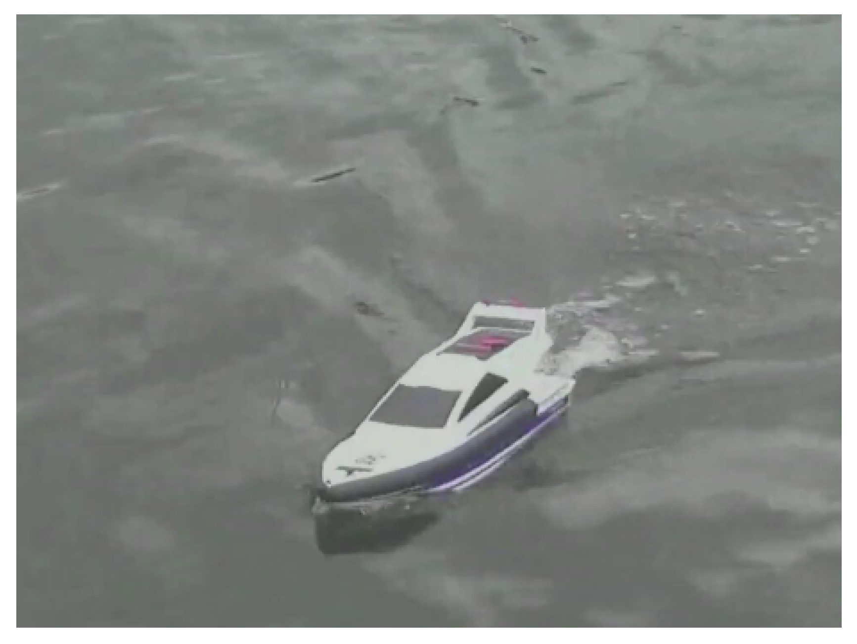
2. Autonomous DDboats

As an experimental platform for the validation of localization algorithms, we used two identical DDboats—see Figure 1—that were originally constructed as a students’ educational platform at ENSTA Bretagne, Brest, France.
These DDboats are equipped with a GPS receiver, as well as with a compass module, that allow for the implementation of a trajectory tracking control procedure. Moreover, these sensor data are used for modeling uncertainties in the motion of both robots in an a posteriori analysis of an experimental trajectory tracking controller and for the derivation of a bounded-error uncertainty model for the sensors in Section 4.

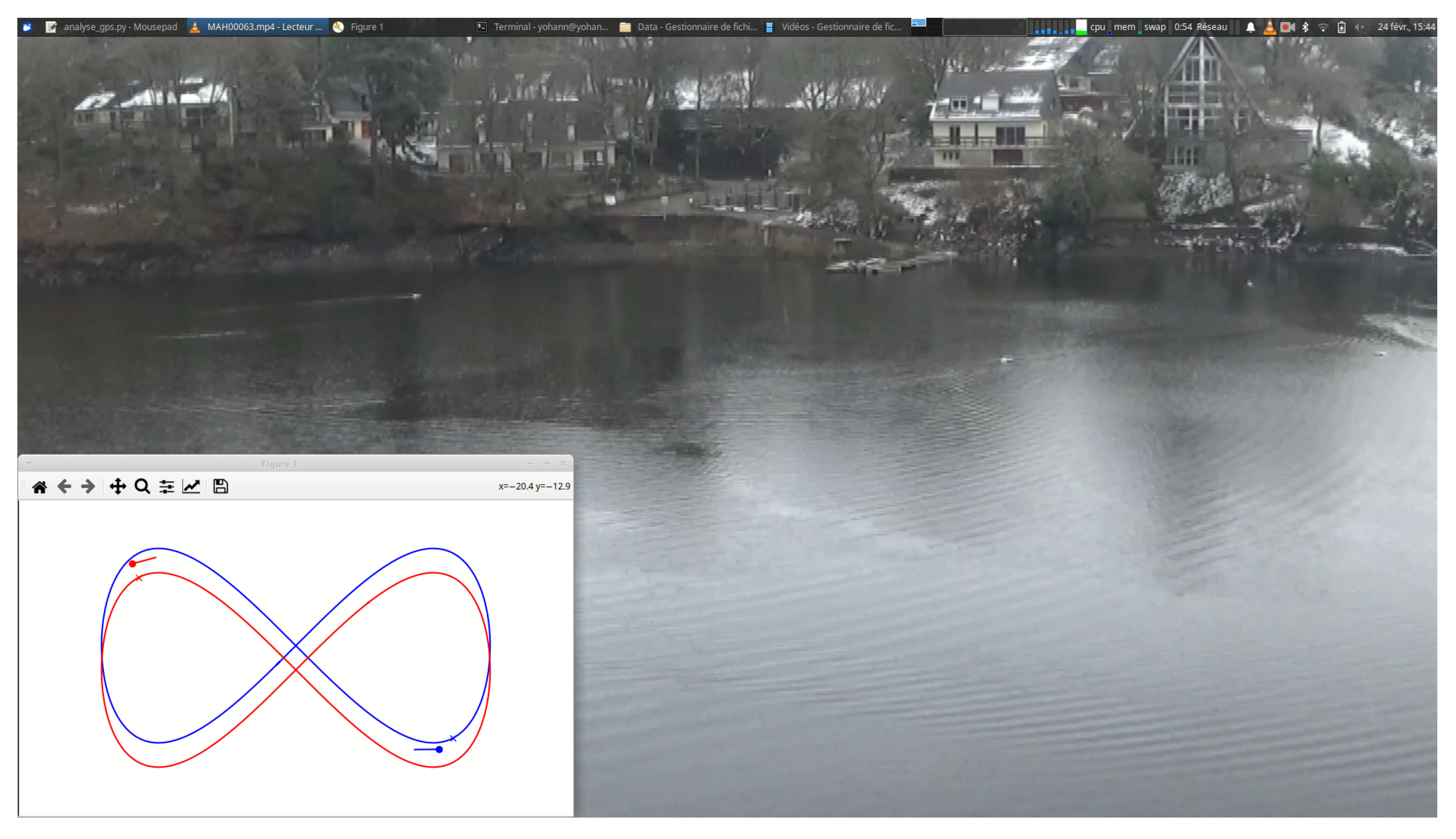
2.1. Specification of Reference Trajectories

The reference trajectories y d i ( t ) of both DDboats i { A , B } are specified in terms of two Lissajous curves
y d A ( t ) = A sin ( 2 α t ) + x 1 , 0 A B sin ( α t ) + x 2 , 0 A
and
y d B ( t ) = A sin ( 2 α t ) + x 1 , 0 B B sin ( α t ) + x 2 , 0 B .
Both curves have the identical shape parameters A = 40 m and B = 20 m . The midpoint positions of these two reference curves are specified by the coordinates
( x 1 , 0 A , y 1 , 0 A ) = ( 35 , 0 ) m and ( x 1 , 0 B , y 1 , 0 B ) = ( 40 , 0 ) m .
For both reference trajectories y d i ( t ) , with the corresponding desired velocities y ˙ d i ( t ) of both DDboats i { A , B } , the period length for completing a full cycle is set to T = 100 s , leading to the velocity parameter α = 2 π T . A graphical representation of these reference trajectories is shown in Figure 2 together with a video snapshot of the experiments in which both DDboats pass through the cycles according to (1) and (2) in opposite directions.

2.2. Tracking Control by Means of an Artificial Potential Field Method

The aforementioned tracking control procedure for both DDboats makes use of an artificial potential field method [18,19,20] to minimize the deviations between the desired trajectories y d i ( t ) and the actual robot positions denoted by the vector x 1 i ( t ) x 2 i ( t ) T . For that purpose, the squared distances between the desired and actual positions are employed as energy-like functions. Computing the temporal derivatives under the assumption of a quasi-stationary boat position and performing a superposition with the desired robot velocities yields the vector-valued input signals
w i ( t ) = γ · y ˙ d i ( t ) · y d i ( t ) x 1 i ( t ) x 2 i ( t ) + y ˙ d i ( t )
for both DDboats i { A , B } .
Here, the heuristically tuned parameter γ > 0 is employed to specify the speed of convergence towards the desired trajectories. The computed vectors w i ( t ) according to (4) determine the desired orientations
ϕ w i ( t ) = arg w i ( t )
of the robots’ force input vectors and the corresponding amplitudes, computed as the Euclidean vector norms
ω i ( t ) = w i ( t ) ,
to specify their required velocities.
Using this information, a proportional-differentiating control law can be established for the propulsion systems of both robots, which consist of a pair of propellers with the rotational speeds u l i ( t ) and u r i ( t ) at the stern of each boat, where the subscripts l and r denote the left and right actuators, respectively.
In such a way, the thrusts of both actuators j { l , r } are given by the saturated input signals
τ j i ( t ) = 0 if τ ˜ j i 0 τ max if τ ˜ j i τ max τ ˜ j i ( t ) else
with
τ ˜ j i ( t ) = K 0 K P , j · ϕ w i ( t ) ϕ i ( t ) + K D , j · ϕ ˙ i ( t ) · ω i ( t ) 2 , j { l , r } ,
where ϕ i ( t ) and ϕ ˙ i ( t ) denote the current headings and angular velocities in a body-fixed coordinate frame of each DDboat. The experimentally tuned gains in (8) satisfy the relations K 0 > 0 , K P , l = K P , r and K D , l = K D , r , respectively.
Finally, the rotational speeds of the actuators are computed as
u l i ( t ) = τ l i ( t ) and u r i ( t ) = τ r i ( t ) .
Despite the fact that this simple control approach does not account for specific measures aiming at a reduction of the influence of external disturbance forces (such as robustifying the controller by means of sliding mode techniques with variable-structure gains chosen so that the worst-case effect of all possible matched uncertainty can be compensated for, or by enhancing the dynamics by means of an observer-based disturbance reduction), Figure 3 shows a quite accurate tracking of the desired trajectories by each of the DDboats. In addition to the position information, GPS- and compass-based heading measurements are also compared with their corresponding desired trajectories in Figure 3. Note that the aim of this control design is not the minimization of tracking errors but rather the implementation of a simple technique to provide experimental data as the input for the following estimation algorithm.
The influence of uncertainty and external disturbances on the actual system dynamics is investigated in detail by the estimation schemes presented in Section 3 and Section 4. In future work, the corresponding estimates cannot only be employed for an a posteriori analysis as shown in this paper, but also in a closed-loop control structure to enhance the accuracy of tracking the reference trajectories y d i in terms of a real-time capable model predictive control approach.

2.3. Modeling of the DDboats

The state and disturbance estimation procedures investigated in Section 3 make use of the following Dubins car model [5] (also often referred to as a simple kinematic car model):
x ˙ 1 i ( t ) x ˙ 2 i ( t ) v ˙ i ( t ) ϕ ˙ i ( t ) z ˙ 1 i ( t ) z ˙ 2 i ( t ) = cos ϕ i ( t ) · v i ( t ) sin ϕ i ( t ) · v i ( t ) u v i ( t ) + z 1 i ( t ) u ϕ i ( t ) + z 2 i ( t ) 0 0
with the state vector
x i ( t ) = x 1 i ( t ) x 2 i ( t ) v i ( t ) ϕ i ( t ) z 1 i ( t ) z 2 i ( t ) T ,
and the effective system inputs u ϕ i ( t ) and u v i ( t ) , as well as the external disturbances z 1 i ( t ) and z 2 i ( t ) , that are included in (10) by means of two independent integrator disturbance models z ˙ 1 i ( t ) = 0 and z ˙ 2 i ( t ) = 0 .

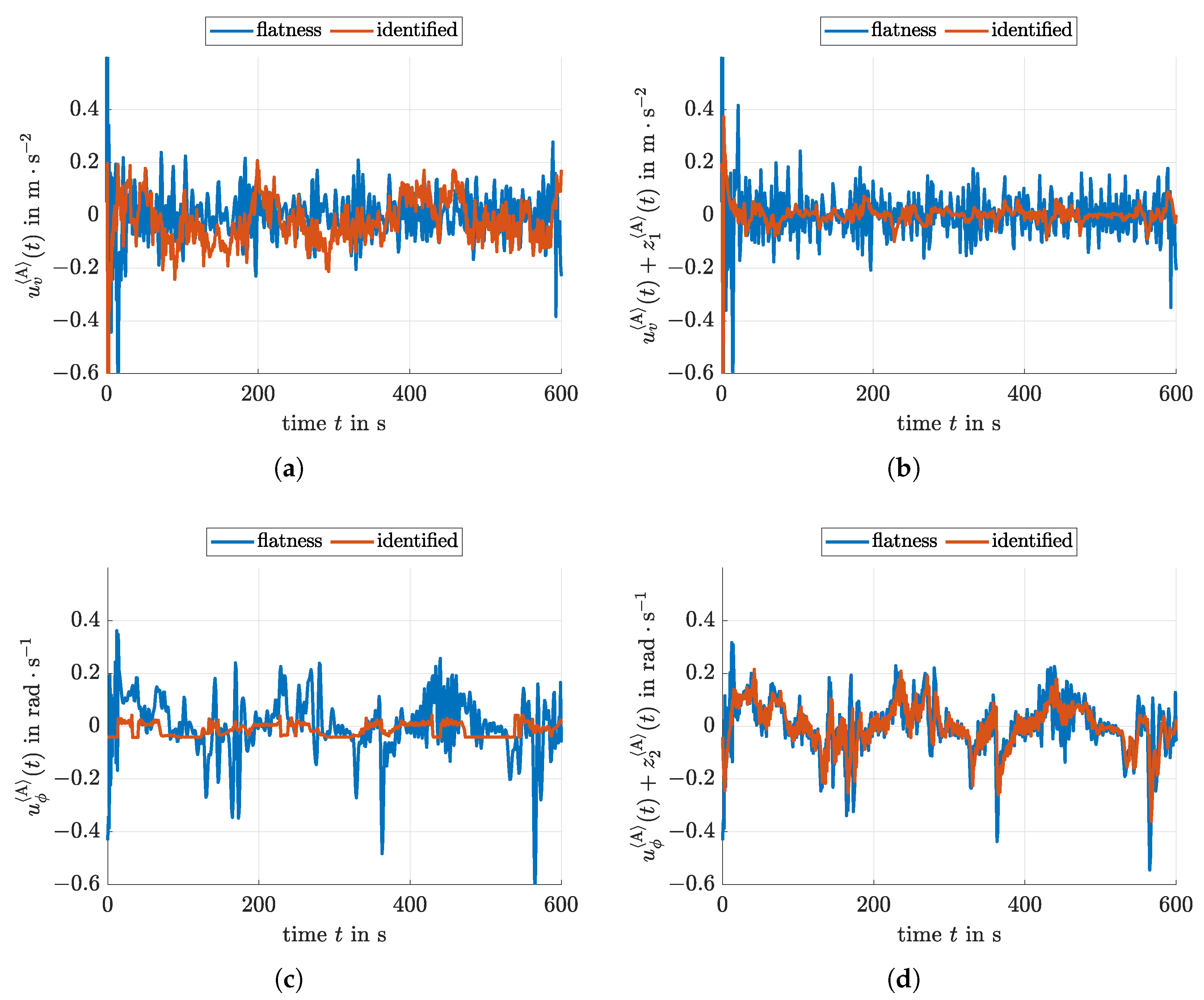
2.3.1. Identified Model-Based Representation of the Effective System Inputs

To account for the knowledge of the control strategy (4)–(9) described in the previous subsection, the effective system inputs in (10) can be specified as
u v i ( t ) = p 1 i · v i ( t ) 2 + p 2 i · u l i ( t ) + u r i ( t ) + p 3 i · u l i ( t ) 2 + u r i ( t ) 2
and
u ϕ i ( t ) = p 4 i · u l i ( t ) u r i ( t ) + p 5 i · u l i ( t ) 2 u r i ( t ) 2 ,
where the parameters p m i , m { 1 , , 5 } , are computed from an offline least-squares identification based on the GPS-based position measurements ( x 1 , m i t , x 2 , m i t ) , the compass information for the ships’ headings ϕ m i ( t ) , and the experimental control signals u l i ( t ) and u r i ( t ) . Required derivatives are determined numerically by using an explicit Euler scheme with a fixed sampling time T s = 1 s .

2.3.2. Signal-Based Representation of the Effective System Inputs

Alternatively, the property of differential flatness [21] of the model (10) can be exploited to approximate the input signals
u v i ( t ) = d x ˙ 1 , m i ( t ) 2 + x ˙ 2 , m i ( t ) 2 d t 1 T s 2 · x 1 , m i t k + 1 x 1 , m i t k 2 + x 2 , m i t k + 1 x 2 , m i t k 2 1 T s 2 · x 1 , m i t k x 1 , m i t k 1 2 + x 2 , m i t k x 2 , m i t k 1 2
and
u ϕ i ( t ) = d ϕ m i ( t ) d t 1 T s · ϕ m i t k + 1 ϕ m i t k
after setting the disturbance inputs z 1 i ( t ) and z 2 i ( t ) to zero with T s = t k + 1 t k .
To avoid the amplification of measurement noise in the following reconstruction of input disturbances, the signals u v i ( t ) and u ϕ i ( t ) are filtered offline (i.e., after the completion of the complete trajectory tracking experiment) by a 12-th order infinite impulse response low pass filter with a cut-off frequency of 0.2 Hz .

2.3.3. A Posteriori Reconstruction of Input Disturbances

To reconstruct the disturbance signals z ^ 1 i ( t ) and z ^ 2 i ( t ) for both alternative input representations described in the preceding two subsections, the state observer
x ^ ˙ i ( t ) = cos ϕ ^ i ( t ) · v ^ i ( t ) sin ϕ ^ i ( t ) · v ^ i ( t ) u v i ( t ) + z ^ 1 i ( t ) u ϕ i ( t ) + z ^ 2 i ( t ) 0 0 + H ( t ) · y m i t C x ^ i ( t ) = 0 0 cos ϕ ^ i ( t ) 0 0 0 0 0 sin ϕ ^ i ( t ) 0 0 0 0 0 0 0 1 0 0 0 0 0 0 1 0 0 0 0 0 0 0 0 0 0 0 0 A x ^ i ( t ) · x ^ ( t ) + 0 0 u v i ( t ) u ϕ i ( t ) 0 0 + H ( t ) · y m i t C x ^ i ( t )
with the output matrix
C = 1 0 0 0 0 0 0 1 0 0 0 0 0 0 1 0 0 0 0 0 0 1 0 0
and the measurement vector y m i t containing the boats’ positions, their velocities, and their headings are employed. The corresponding output estimates are, hence, denoted by C x ^ i ( t ) . The computation of the gain matrix H exploits the duality principle between control and observer design (which is motivated by the quasi-static extended Kalman filter design according to [5]) in terms of solving the algebraic Riccati equation
P x ^ i · C T · R 1 · C · P x ^ i A x ^ i · P x ^ i P x ^ i · A T x ^ i Q = 0
in each sampling instant t k at which measured data y m t are available. As a scheduling parameter, the most recent state estimate x ^ is used in (18) as the argument of the state-dependent system matrix A x ^ i .
Note that this continuous-time observer design is applicable due to the short temporal distance ( T s = 1 s ) between two subsequent measurement instants and the comparably small variation in the state variables over a single discretization interval. The temporally varying observer gain
H ( t ) = P x ^ i · C T · R 1
is recomputed in each sampling instant (due to the a posteriori application for the purpose of identifying process uncertainty, this recomputation does not impose any constraints concerning real-time applicability) for the heuristically chosen weighting matrices
Q = diag 200 200 100 100 10 10 and R = diag 0.1 0.1 0.1 0.25 .
For a stochastic interpretation of these matrices in terms of the covariances of process and measurement noise, see [14,15].
With the help of this observer and the effective input estimates according to the preceding two subsections, the results depicted in Figure 4 are obtained. Table 1 summarizes the standard deviations for each of the components of the vector H ( t ) · y m i t C x ^ i ( t ) over the complete horizon of the trajectory tracking experiment. These standard deviations are used in Section 4.1 to define interval bounds for an additive process noise acting independently on each component of the state equations.

3. Ellipsoidal State Estimation Procedure

For the description of the ellipsoidal state estimation procedure, assume that a discrete-time system model in the form
x k + 1 = Φ p · x k + ψ p
is given, where Φ p is the system matrix and ψ p is a bounded disturbance or control input. Although discrete-time system models are considered in this paper, the term ψ p can also be used to account for time discretization errors of continuous-time models. A corresponding approach has recently been investigated in [22]. Due to the fact that time discretization errors are much smaller for the application at hand in comparison with the process noise discussed in the previous section, the further derivation of the ellipsoidal state estimation approach is restricted solely to the discrete-time setting.
Both Φ p and ψ p may depend on uncertain parameters p R n p . These parameters may also reflect state dependencies in the system matrix and the input vector if a nonlinear set of state equations is reformulated according to [4] into a quasi-linear form, cf. (16).
In both cases (either pure parameter dependencies and/or state dependencies), the vector p = p 1 p n p T is assumed to be piecewise constant between two subsequent sampling instants and bounded in terms of a set-valued uncertainty model by the axis-aligned multi-dimensional interval box p p = p ¯ ; p ¯ , where the element-wise relation p i p i p ¯ i holds for each component i { 1 , , n p } of the parameter vector.
The ellipsoidal state estimation procedure applied in this paper is obtained as a special case of the thick ellipsoid state estimation presented in [4]. To implement this procedure, we assume that the additive term ψ p is included in a suitable ellipsoid that—in the case of an initial box-valued enclosure—is obtained by enclosing the additive bounded uncertainty in its associated Löwner–John ellipsoid [23].
In general, ellipsoidal state bounds at the time instant k are denoted as
E k μ k , Γ k : = x k R n | x k μ k T Γ k T Γ k 1 x k μ k 1
for which the shape matrix is given in the factorized form Q k = Γ k Γ k T 0 with the positive definite matrix Q k . This matrix specifies—depending on the following estimation steps—state domains before the evaluation of a prediction step, or the corrected state estimates after the evaluation of the associated measurement update step. Moreover, denote the ellipsoid midpoint as μ k R n .
In addition to the dynamic system model (21), the measured system outputs y m , k = y m ( t k ) are described by an ellipsoidal uncertainty representation in the form
C · x k + 1 y m , k + 1 T · Q m 1 · C · x k + 1 y m , k + 1 1 ,
where Q m is the shape matrix defining outer bounds for the measurement uncertainty.
To make the ellipsoidal set intersection operator introduced in [4] applicable for the state estimation task, the expression (23) is reformulated equivalently in terms of the inequality constraint
x k + 1 y m , k + 1 T · P m · x k + 1 y m , k + 1 1 .
In this inequality (24), the matrix P m is a purely diagonal matrix if the system’s output matrix C in (23) represents a direct measurement of selected components of the state vector x k + 1 . If a smaller number of outputs than state variables are available in this case, the matrix P m is not invertible and represents a degenerate ellipsoid in the n-dimensional state space; see also [4,12].
Using this notation, entries in the vector y m , k + 1 that correspond to non-measured components of the state vector at the time instant k + 1 are set to the associated ellipsoid midpoint μ k + 1 obtained from the state prediction, while all other components correspond to the point-valued measured data y m , k + 1 .

3.1. Ellipsoidal State Prediction Step

The first three steps of the following state prediction procedure for discrete-time systems (21) were basically published and proven in [4]. The major difference is that the quoted publication made use of a thick ellipsoid state enclosure approach in which inner and outer ellipsoid bounds for the first term Φ p · x k in (21) were determined simultaneously.
However, for the sake of a pure state estimation in the form of computing guaranteed outer enclosures, only the outer bounds of those so-called thick ellipsoids are of interest. For that reason, the approach from [4] is simplified by leaving out the computation of the associated inner state bounds.
For finding outer ellipsoidal enclosures of the subexpression Φ p · x k in (21), we assume that this part of the system model is reformulated in the form
x Φ , k + 1 = Φ p · x k = Φ p · x ˇ k + Φ ˜ · μ k + Φ p Φ ˜ · μ k .
This allows for propagating an origin-centered ellipsoid with the help of the first term in (25), while the remaining terms account for the influence of the generally non-zero ellipsoid midpoint. For that purpose, introduce the following notation already applied in (25) and further used during the state prediction consisting of the Steps P1–P5:
E k = E k μ k , Γ k denotes the uncertainty on the non - origin centered states x k ,
E ˇ k = E ˇ k 0 , Γ k the uncertainty of x ˇ k after shifting the ellipsoid to the origin , and
Φ ˜ = Φ mid p the midpoint approximation of the quasi - linear system matrix with
p p = p ¯ ; p ¯ , and the interval midpoint mid p = 1 2 · p ¯ + p ¯ .
Step P1:
Apply
x ˇ k + 1 = Φ p · x ˇ k
to the ellipsoid E ˇ k in (27). The shape matrix of the outer ellipsoid enclosure of the image set is described by an ellipsoid with the shape matrix
Q ˇ k + 1 = α k + 1 2 · Γ k + 1 · Γ k + 1 T ,
where α k + 1 0 is the smallest value for which the linear matrix inequality
M k + 1 : = Λ Q k 1 Φ T p · Φ ˜ T Φ ˜ 1 · Φ p α k + 1 2 R k Λ 0 , Q k = Γ k · Γ k T
is satisfied for all p p with
R k : = Γ k · Γ k T .
In (32), the preconditioning matrix Λ = blkdiag β I , β 1 I is defined with the help of the identity matrix I R n × n and the square root β = min { λ i Q k } of the smallest eigenvalue of Q k as described in [22]. This choice helps to prevent unnecessarily conservative state bounds in cases in which the norms of Φ ˜ 1 · Φ p and Q k are significantly different.
Step P2:
Compute interval bounds for the term
b k = Φ p Φ ˜ · μ k b k ,
which accounts for a non-zero ellipsoid midpoint with x k , Φ ˜ , and p defined according to (26), (28), and (29). Inflate the outer ellipsoid bound described by the shape matrix (31) with
Q k + 1 = 1 + ρ O , k + 1 2 · Q ˇ k + 1 and ρ O , k + 1 = sup α k + 1 1 · Γ k 1 · b k .
For a definition of the interval-valued generalization of the Euclidean norm operator, see [12].
Step P3:
Compute the updated ellipsoid midpoint as
μ Φ , k + 1 = Φ ˜ · μ k .
The outer ellipsoidal enclosure E Φ , k + 1 of x Φ , k + 1 at the time instant k + 1 then becomes
x Φ , k + 1 E Φ , k + 1 μ Φ , k + 1 , Γ Φ , k + 1 ,
where
Γ Φ , k + 1 = α k + 1 · 1 + ρ O , k + 1 · Φ ˜ · Γ k .
Step P4:
Determine an ellipsoidal enclosure (the aforementioned Löwner–John ellipsoid) for the summand
x Ψ , k + 1 = ψ p
according to
x Ψ , k + 1 E Ψ , k + 1 μ Ψ , k + 1 , Γ Ψ , k + 1 .
To determine this ellipsoid from an interval vector ψ p with the corresponding vertices x Ψ j , j { 1 , , L } , where
Q Ψ , k + 1 = Γ Ψ , k + 1 · Γ Ψ , k + 1 T
holds, the minimum-volume Löwner–John ellipsoid is determined by solving the linear matrix inequality constrained optimization problem
min Q Ψ , k + 1 , μ Ψ , k + 1 trace Q Ψ , k + 1 1 x Ψ , k + 1 j μ Ψ , k + 1 T x Ψ , k + 1 j μ Ψ , k + 1 Q Ψ , k + 1 0 for all j { 1 , , L } Q Ψ , k + 1 0 .
Further details concerning these inequality constraints, the choice of the number of vertices L, and a simplified version purely based on interval analysis are discussed in [12]. Moreover, note that the exact volume minimization task would require the solution of an optimization task in which a complex determinant minimization task is involved. This task is replaced by the minimization of a matrix trace as described in Appendix C of [24]. Due to the linearity of the trace operator (and its close-to-optimal behavior), this version is used for the proposed ellipsoid prediction step when determining the bounds E Ψ , k + 1 .
Step P5:
Compute an ellipsoidal enclosure of the Minkowski sum of the two intermediate results E Φ , k + 1 and E Ψ , k + 1 according to
E Φ , k + 1 E Ψ , k + 1 E k + 1 μ k + 1 , Γ k + 1
with the new midpoint
μ k + 1 = μ Φ , k + 1 + μ Ψ , k + 1
and the updated shape matrix
Γ k + 1 = Q k + 1 1 2 ,
resulting from the closed-form expression
Q k + 1 = 1 + 1 β · Γ Φ , k + 1 · Γ Φ , k + 1 T + 1 + β · Γ Ψ , k + 1 · Γ Ψ , k + 1 T
with
β = trace Γ Φ , k + 1 · Γ Φ , k + 1 T trace Γ Ψ , k + 1 · Γ Ψ , k + 1 T .
For a derivation of this expression, the reader is referred to  [7,25,26].

3.2. Ellipsoidal Measurement Update Step

To perform the ellipsoidal measurement update step, we employ the intersection technique for ellipsoids with different midpoints that was derived in [4]. This approach is an extension of the computation of Dikin ellipsoids, which is discussed in detail in [27].
This extension consists of the following two steps:
Step C1:
Determine the common center point for the bounds of the intersection, where the center point must be included in all ellipsoids to be intersected;
Step C2:
Determine the shape matrices for the outer ellipsoid bound according to the computation of Dikin ellipsoids according to [27].
Preliminary work in [4] has shown that an efficient heuristic approach for the computation of the common center point μ ˜ k + 1 in Step C1 of the two ellipsoids E μ k + 1 , Γ k + 1 , Q k + 1 = Γ k + 1 Γ k + 1 T and E μ m , k + 1 , Γ m , k + 1 , Q m , k + 1 = Γ m , k + 1 Γ m , k + 1 T is given by an approach motivated by the innovation step of a Kalman filter [14,28].
Here, the ellipsoid E μ m , k + 1 , Γ m , k + 1 characterizes the measurement model (23) with the output matrix C .
With the help of this information, the Kalman gain matrix
L k + 1 = Q k + 1 · C T · C · Q k + 1 · C T + Q m , k + 1 1
is computed. Then, the updated ellipsoid midpoint results in
μ ˜ k + 1 = μ k + 1 + L k + 1 · μ m , k + 1 μ k + 1 .
Both ellipsoids to be intersected are first enclosed during Step C2 by new ellipsoids centered at the midpoint μ ˜ k + 1 . For that purpose, the scaling factors
ζ k + 1 = 1 + Δ μ 1 , k + 1 with Δ μ 1 , k + 1 = Q k + 1 1 2 · μ ˜ k + 1 μ k + 1
and
ζ m , k + 1 = 1 + Δ μ m , k + 1 with Δ μ m , k + 1 = P m 1 2 · μ ˜ k + 1 μ m , k + 1
are determined, which represent the maximum distances of the new midpoint computed in Equation (49) from the original ellipsoid surfaces. Here, Δ μ · , k + 1 is the Euclidean norm of the corresponding vector-valued argument.
Second, the outer bound of the intersection of these two rescaled ellipsoids is given by Equation (53) in [4] by
E k + 1 = E k + 1 μ ˜ k + 1 , Γ k + 1 with Γ k + 1 = Q k + 1 1 2 ,
where the shape matrix is determined with the closed-form expression
Q k + 1 = 4 · 2 · ζ k + 1 2 · Q k + 1 1 + ζ m , k + 1 2 · P m 1
with Q k + 1 from (35). As shown in [4], this approach is applicable also in cases in which not all components of the state vector are measured, i.e., if the matrix P m introduced in (24) represents a degenerate ellipsoid with bounds that may be infinitely wide in some components of the state space. Although this procedure may be less accurate than the technique presented in [8,29], it is preferred in this paper due to its simplified closed-form solution representation and because it avoids the online solution of linear matrix inequalities.

4. Modeling of Uncertainty

The ellipsoidal state estimation technique discussed in this paper relies on suitable uncertainty models for both bounded process and measurement noise. This section gives an application-driven description on how suitable bounds can be derived for real-life system models. To perform the parameterization of the uncertainty models, we rely on the identification experiments and measured data summarized in Section 2.

4.1. Uncertainty in the Dynamic System Model: Bounded Process Noise

In Equation (10), the control inputs of the DDboats under consideration have been described by u v i ( t ) + z 1 i ( t ) and u ϕ i ( t ) + z 2 i ( t ) as a superposition of an identified or flatness-based input term and a corresponding point-valued disturbance estimate.
With this knowledge, the ellipsoidal state estimation can be applied to a discrete-time system model (discretization step size T s = 1 s , corresponding to the sampling time of the available GPS sensor) with the state vector
x k i : = x i ( t k ) = x 1 i ( t k ) x 2 i ( t k ) v i ( t k ) ϕ i ( t k ) T , i { A , B } .
For the sake of a compact notation of the scheme for uncertainty modeling, the superscript · i is omitted in the following equations as long as this does not lead to ambiguities.
Using an explicit Euler discretization for the continuous-time state equations, which is sufficiently accurate due to the small sampling time T s and volume-preserving according to [5] for a Dubins car model, the system model
x ( t k + 1 ) = 1 0 T s cos ϕ ( t k ) 0 0 1 T s sin ϕ ( t k ) 0 0 0 1 0 0 0 0 1 Φ p · x ( t k ) + T s · 0 0 u v ( t k ) + z ^ 1 ( t k ) u ϕ ( t k ) + z ^ 2 ( t k ) + w ( t k ) Ψ p
is obtained. This model has the same form as the system model (21) that was used for the derivation of the ellipsoidal state estimation procedure in the previous section. To account for uncertainty in the process dynamics, the term Ψ p needs to be bounded by an ellipsoid E Ψ , k + 1 μ Ψ , k + 1 , Γ Ψ , k + 1 according to the definition (40).
For the application at hand, this term contains the influence of the control inputs u v ( t k ) and u ϕ ( t k ) and the actuator uncertainties z ^ 1 ( t k ) and z ^ 2 ( t k ) , as well as the disturbance estimates
w ( t k ) = T s · C · H ( t k ) · y m t k C x ^ ( t k )
determined by the observer-based a posteriori uncertainty analysis according to Section 2.3.3.
In this section, these quantities have been determined in a point-valued form with the estimated state vector x ^ ( t ) of the observer (16), where the associated output matrix C is defined in (17).
To make the ellipsoidal estimation scheme applicable, the point-valued estimates are employed as the midpoint vector
μ Ψ , k + 1 = T s · 0 0 u v ( t k ) + z ^ 1 ( t k ) u ϕ ( t k ) + z ^ 2 ( t k ) + w ( t k )
of the ellipsoidal disturbance enclosure. The bounds for axis-aligned disturbance intervals are derived from the standard deviations listed in Table 1. If the parameter r > 0 in
γ l = r · σ x l , l { 1 , , 4 } ,
is employed as a user-defined degree of freedom to specify a desired confidence level of the ellipsoidal disturbance representation, the factorized shape matrix of the process noise term Ψ p results in the (in this example, time-invariant and purely diagonal) expression
Γ Ψ , k + 1 = 2 · T s · diag γ 1 γ 4 ,
being equivalent to
Q Ψ , k + 1 = 2 · r 2 · T s 2 · diag σ x 1 2 σ x 4 2 .
Remark 1.
In Section 5, the heading dependence of the system matrix Φ p in (55) is taken into account in two alternative forms. Firstly, these dependencies are treated as a pure state dependence, where corresponding outer bounds are determined by the proposed estimation algorithm. Second, the set-based heading identification according to the following subsection is taken into account additionally to intersect the estimated bounds with the measurement-based tolerances. This intersection enhances the knowledge on the system dynamics and hence reduces the uncertainty included in the set-valued bounds on the system matrix Φ p .
Remark 2.
If an a posteriori (observer-based) identification of the disturbance terms z 1 ( t ) and z 2 ( t ) were not possible, their influence would have to be described by means of conservative worst-case bounds. They have to be included in the terms (58) by inflating the corresponding standard deviations σ x l .

4.2. Quantification of Measurement Uncertainty: Bounded Measurement Noise

To identify a set-valued uncertainty model for the compass sensor, as well as for the GPS-based position measurements, independently for each of the DDboats, assume additive, time-varying interval uncertainties in the model for the compass sensor
ϕ t k ϕ m t k + Δ ϕ t k
as well as time-invariant uncertainty bounds for the GPS-based position measurement according to
x 1 t k x 2 t k x 1 , m t k x 2 , m t k + Δ x 1 Δ x 2 .
A corresponding uncertainty representation of the velocity vectors of the DDboats is obtained by an explicit Euler method-based approximation in the form
v 1 t k v 2 t k 1 T s · x 1 , m t k + 1 x 2 , m t k + 1 x 1 , m t k x 2 , m t k + Δ x ˜ 1 Δ x ˜ 2 ,
where, under the assumption of symmetric intervals Δ x 1 Δ x 2 T 0 , the error bounds
Δ x ˜ 1 Δ x ˜ 2 = 2 · Δ x 1 Δ x 2
of the velocity model (63) are obtained.
A contractor-based identification of the interval bounds Δ ϕ t k , Δ x 1 , and Δ x 2 has to make sure that, for a reasonable initial search space for the measurement uncertainties, the compatibility constraint
tan ϕ m t k + Δ ϕ t k x 2 , m t k + 1 x 2 , m t k + Δ x ˜ 2 x 1 , m t k + 1 x 1 , m t k + Δ x ˜ 1
is satisfied at each measurement instant t k , where—in this equation—we assume for ease of notation that the denominator term in brackets does not include the value zero.
A comparison of the point-valued measurements according to Figure 3c,d motivates the initialization of Δ ϕ t k = 0.6 · 1 ; 1 rad (lower and upper interval bounds are separated by semi-colons to distinguish them from vectors, which are also typeset by using square brackets). These graphs correspond equally to the measurement models (61) as well as to atan 2 v 2 , v 1 with the velocity components defined in (63), in which, all uncertainty intervals would be zero in the noise-free setting.
Moreover, the worst-case GPS uncertainty is set to the independent intervals Δ x 1 = 2 ; 2 m and Δ x 2 = 2 ; 2 m . Using this initialization, Algorithm 1 is used to contract the error bounds so that the constraint (65) is satisfied.
Algorithm 1: Contractor-based sensor calibration.
  • initialize the interval bound Δ ϕ t k
  • initialize the interval bounds Δ x ˜ 1 and Δ x ˜ 2
  • exclude all samples k, where 0 tan ϕ m t k + Δ ϕ t k
  • exclude all samples k, where tan ϕ m t k + Δ ϕ t k = = NaN
  • include all remaining samples k in the set K
  • while TRUE do
  •    Contractor for Δ x ˜ 1 :
  •     Δ x ˜ 1 = k K x 2 , m t k + 1 x 2 , m t k + Δ x ˜ 2 tan ϕ m t k + Δ ϕ t k x 1 , m t k + 1 x 1 , m t k Δ x ˜ 1
  •    generate symmetric bounds Δ x ˜ 1 : = 1 ; 1 · max inf Δ x ˜ 1 , sup Δ x ˜ 1
  •    Contractor for Δ x ˜ 2 :
  •     Δ x ˜ 2 = k K ( x 1 , m t k + 1 x 1 , m t k + Δ x ˜ 1 · tan ϕ m t k + Δ ϕ t k
  •     x 2 , m t k + 1 x 2 , m t k ) Δ x ˜ 2
  •    generate symmetric bounds Δ x ˜ 2 : = 1 ; 1 · max inf Δ x ˜ 2 , sup Δ x ˜ 2
  •    Contractor for Δ ϕ t k for all k K :
  •     Δ ϕ t k : = Δ ϕ t k
  •     atan 2 x 2 , m t k + 1 x 2 , m t k + Δ x ˜ 2 , x 1 , m t k + 1 x 1 , m t k ϕ m t k
  •    if  any Δ ϕ t k = = NaN  then
  •      reset Δ x ˜ 1 and Δ x ˜ 1 to initial bounds
  •      inflate the bounds for Δ ϕ t k
  • else if no further contractance of interval bounds possible then
  •      break
  •    end if
  • end while
  • set Δ x 1 : = 0.5 · Δ x ˜ 1 and Δ x 2 : = 0.5 · Δ x ˜ 2
  • return Δ x 1 , Δ x 2 , and Δ ϕ t k
Remark 3.
This algorithm can be simplified by imposing identical bounds Δ ϕ t k for all time steps t k . In this case, we deactivate the contractor for the angle uncertainty Δ ϕ t k and perform an inflation of this value at all time steps if the condition any Δ ϕ t k = = NaN becomes active.
Remark 4.
An interval extension of the atan 2 function is described in [30]. A straightforward extension of a phase unwrap operation applied individually to all interval bounds of the generalized atan 2 function in the case of angles leaving the interval π ; π allows for determining the depicted enclosures in Figure 5.
Figure 5 gives a comparison of the reconstructed bounds for the compass-based heading measurements, as well as for the reconstruction of the uncertainty in the heading angle using the GPS-based velocity estimate for both DDboats, without and with the assumption of time-varying uncertainty Δ ϕ i t k .
Table 2 gives an overview of characteristic values for the identified measurement uncertainty in terms of the mean interval radii
0.5 · sup Δ ϕ t k i inf Δ ϕ t k i
of the angle estimates for the DDboats i { A , B } , both for the compass-based and the GPS-based data, as well as the suprema of the symmetric intervals for the GPS position accuracy.
Since the time-varying model leads to significantly better bounds on the reconstruction of the uncertainties, we restrict ourselves in the following investigation to the time-varying model according to Figure 5b,d, where the intersection of the intervals for the compass sensor and the GPS-based heading intervals according to Figure 6 is employed by the ellipsoidal state observer. Velocity measurement intervals result from a direct use of Definition (63), into which, the bounds for the position errors are directly substituted. In view of the fact that the estimate for the GPS accuracy may be biased because of the specific form of the employed Lissajous-shaped trajectory with different elongations in the x 1 and x 2 coordinates, the boldface values (as the largest entries in both coordinates) serve as the values for parameterizing the uncertainty model of both x 1 and x 2 .

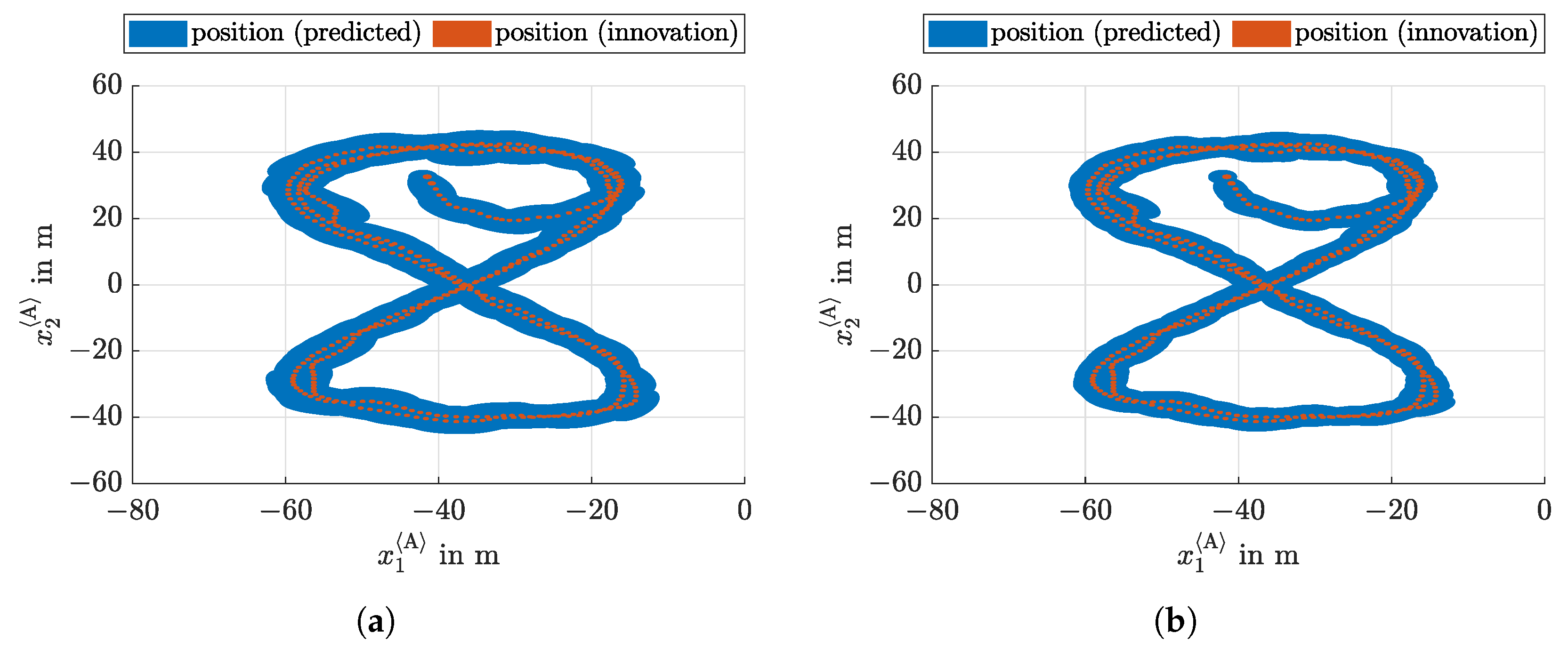
5. Estimation Results

This section presents various estimation results when using the proposed ellipsoidal enclosure technique based on an a posteriori evaluation of the measured data for both DDboats A and B. Here, we distinguish the localization of the DDboats without and with using information on the measured heading. In all presented results, the confidence parameter r = 3 is used in Equations (58)–(60).

5.1. Localization without Heading Measurement

Figure 7 gives a comparison of the localization results after the ellipsoidal state prediction step, as well as after the subsequent set-based innovation step. It can be seen that the additional use of velocity information, represented by the interval data described in Section 4.2, only slightly improves the estimation accuracy in comparison with a pure position measurement.
It has to be pointed out that the heading angle included as the fourth state variable in the model (55) is unobservable if only the coordinates x 1 and x 2 are measured by the available GPS. For that reason, a countermeasure against an unbounded growth of the uncertainty in the heading angle information needs to be included as a virtual measurement in the ellipsoidal innovation stage. This restriction has been set to the interval π ; π rad in both subgraphs of Figure 7, while the velocity was further restricted in Figure 7a to an interval 2 ; 2 m s , centered around the midpoint of the current state prediction.
Remark 5.
In future work, further quasi-linear state-space representations (also ensuring observability of the heading for non-vanishing boat velocities based on position measurements) can be included in the estimation procedure. These reformulated system models may also serve as virtual measurement generators.
The corresponding analytical reformulations of the system model (55) split up the term sin ϕ ( t k ) · v ( t k ) into the form
sin ϕ ( t k ) · v ( t k ) = 0 0 α · sin ϕ ( t k ) 1 α · sin ϕ ( t k ) ϕ ( t k ) · v ( t k ) · x t k
with α R as an optimization degree of freedom. The optimal choice of this parameter α is currently being investigated in a parallel research activity aiming at the use of an ellipsoidal calculus for analyzing the stability of discrete-time dynamic systems, as well as for extensions of the control procedure presented in [31].

5.2. Localization with Heading Measurement

An enhancement of the estimation quality becomes possible as soon as the interval data for the measured heading are additionally included in the estimation procedure. The corresponding results are shown in Figure 8a, where no significant differences between the direct use of the measured heading intervals in the system matrix of the state-space representation in (55) and its replacement by the estimated heading bounds are visible.
Note that, in both Figure 7 and Figure 8, the measurements are assumed to be available at each sampling time instant of the discrete-time system model, where measurements of all four state variables are used in Figure 8, in contrast to the specified subsets in Figure 7.
A reduction in the measurement frequency is analyzed in Figure 9. There, it becomes obvious that the use of measured heading information in the evaluation of the system matrix in (55) leads to much tighter state enclosures than the use of purely predicted heading bounds. Here, it has been assumed that the duration between two subsequent measurements corresponds to 3 T s . The fact that the use of the measured heading information in the evaluation of the system matrix during the state prediction step significantly reduces the width of the predicted state bounds gives rise to the following practical recommendation if low-cost sensors and computing hardware are used: to be able to reduce the sampling frequency of the GPS, while still obtaining sufficiently tight position bounds for the vessel after the prediction step under consideration of large external disturbances as in this paper, it is reasonable to provide compass-based heading information with higher sampling frequencies, even though their tolerance bounds may not be especially tight.
Moreover, event-triggered state estimation procedures can be implemented in future work on the basis of the widths of the predicted vessel position, which request new state measurements as soon as the volume of the predicted ellipsoids exceeds a user-defined threshold value.

5.3. Proof of Collision Avoidance

As a final evaluation step, the position estimates according to Figure 8a are used to compute interval bounds for the distance of both boats that performed a synchronized motion during the measurement experiment. For this purpose, an interval-based distance computation is performed after enclosing the position ellipsoids into tight axis-aligned interval boxes. If this computation is performed purely on the basis of the predicted state information—see Figure 10—there exist some time intervals during the experiment in which a collision of the two boats cannot be ruled out with certainty (the value zero is included as the lower interval bound of the computed distances).
Requesting the GPS position measurement during these phases and using the results of the innovation stage as shown in the previous subsection shows that the experiment from which the measurements were obtained is fully safe and that collisions of both boats can be ruled out with certainty within the considered bounds on the measurement uncertainty and the external disturbances identified in Section 4. As already mentioned in the previous subsection, an event-triggered estimation scheme can be used here as well to tighten the position bounds as soon as both boats approach each other and the predicted infima of the interval-based distance forecast fall below a specific threshold value.

6. Conclusions and Outlook on Future Work

In this paper, a novel ellipsoidal state estimation procedure was validated experimentally for real-life measurements from the area of marine applications. It was shown that a set-valued uncertainty modeling can be used to characterize the influence of external disturbances acting on a vessel. Moreover, an interval approach was shown that allows for characterizing the accuracy of GPS-based measurements, in combination with a fusion with a compass-based counterpart. Using all of these information sources, an ellipsoidal state estimation procedure was implemented that allows for estimating worst-case outer bounds of the reachable position of a ship and proving the safety of specific maneuvers with respect to collision avoidance.
In future work, further quasi-linear system models will be investigated to improve observability and to combine numerous system formulations to tighten the result of the state prediction step. Moreover, the presented work represents the basis for the development of event-triggered state estimation procedures that only perform innovation stages as soon as certain indicator functions become active, such as the volumes of the predicted state ellipsoids exceeding certain thresholds or objects coming closer to an obstacle than a certain minimum safety distance. In addition, combinations of set-valued and stochastic uncertainty models will be investigated to establish mixed uncertainty representations. There, ellipsoidal state enclosures can serve as a representation for certain stochastically motivated confidence levels. Finally, it is desired to use the proposed estimation scheme for the implementation of set-based model-predictive control procedures for uncertain nonlinear dynamic systems.

Author Contributions

The ellipsoidal enclosure technique was developed by A.R. and L.J. All experiments were performed by Y.G., K.L. and B.H. under the supervision of L.J. The estimation approach was reviewed by J.R., S.W. and P.H. The paper was jointly written by all authors. All authors have read and agreed to the published version of the manuscript.

Funding

This research received no external funding.

Institutional Review Board Statement

Not applicable.

Informed Consent Statement

Not applicable.

Data Availability Statement

Data are contained within the article.

Conflicts of Interest

The authors declare no conflict of interest.

References

  1. Fossen, T. Handbook of Marine Craft Hydrodynamics and Motion Control, 2nd ed.; Wiley: Hoboken, NJ, USA, 2021. [Google Scholar]
  2. Xue, Y.; Liu, Y.; Xue, G.; Chen, G. Identification and Prediction of Ship Maneuvering Motion Based on a Gaussian Process with Uncertainty Propagation. J. Mar. Sci. Eng. 2021, 9, 804. [Google Scholar] [CrossRef]
  3. Mayer, G. Interval Analysis and Automatic Result Verification; De Gruyter Studies in Mathematics; De Gruyter: Berlin, Germany; Boston, MA, USA, 2017. [Google Scholar]
  4. Rauh, A.; Bourgois, A.; Jaulin, L. Union and Intersection Operators for Thick Ellipsoid State Enclosures: Application to Bounded-Error Discrete-Time State Observer Design. Algorithms 2021, 14, 88. [Google Scholar] [CrossRef]
  5. Rauh, A.; Jaulin, L. A Computationally Inexpensive Algorithm for Determining Outer and Inner Enclosures of Nonlinear Mappings of Ellipsoidal Domains. Int. J. Appl. Math. Comput. Sci. AMCS 2021, 31, 399–415. [Google Scholar]
  6. Houska, B.; Villanueva, M.; Chachuat, B. Stable Set-Valued Integration of Nonlinear Dynamic Systems using Affine Set-Parameterizations. Siam J. Numer. Anal. 2015, 53, 2307–2328. [Google Scholar] [CrossRef] [Green Version]
  7. Kurzhanskii, A.B.; Vályi, I. Ellipsoidal Calculus for Estimation and Control; Birkhäuser: Boston, MA, USA, 1997. [Google Scholar]
  8. Becis-Aubry, Y. Ellipsoidal Constrained State Estimation in Presence of Bounded Disturbances. 2020. Available online: arxiv.org/pdf/2012.03267v1.pdf (accessed on 13 March 2022).
  9. Rego, B.S.; Scott, J.K.; Raimondo, D.M.; Raffo, G.V. Set-Valued State Estimation of Nonlinear Discrete-Time Systems with Nonlinear Invariants Based on Constrained Zonotopes. Automatica 2021, 129, 109638. [Google Scholar] [CrossRef]
  10. Berz, M.; Makino, K. Verified Integration of ODEs and Flows Using Differential Algebraic Methods on High-Order Taylor Models. Reliab. Comput. 1998, 4, 361–369. [Google Scholar] [CrossRef]
  11. Bünger, F. A Taylor Model Toolbox for Solving ODEs Implemented in MATLAB/INTLAB. J. Comput. Appl. Math. 2020, 368, 112511. [Google Scholar] [CrossRef]
  12. Rauh, A.; Rohou, S.; Jaulin, L. An Ellipsoidal Predictor–Corrector State Estimation Scheme for Linear Continuous-Time Systems with Bounded Parameters and Bounded Measurement Errors. Front. Control Eng. 2022, 3, 785795. [Google Scholar] [CrossRef]
  13. Kühn, W. Rigorous Error Bounds for the Initial Value Problem Based on Defect Estimation. Technical Report. 1999. Available online: http://www.decatur.de/personal/papers/defect.zip (accessed on 6 March 2022).
  14. Stengel, R. Optimal Control and Estimation; Dover Publications, Inc.: Mineola, NY, USA, 1994. [Google Scholar]
  15. Anderson, B.D.O.; Moore, J.B. Optimal Filtering; Dover Publications, Inc.: Mineola, NY, USA, 2005. [Google Scholar]
  16. Hashim, H.A. A Geometric Nonlinear Stochastic Filter for Simultaneous Localization and Mapping. Aerosp. Sci. Technol. 2021, 111, 106569. [Google Scholar] [CrossRef]
  17. Borisov, A.; Bosov, A.; Miller, B.; Miller, G. Passive Underwater Target Tracking: Conditionally Minimax Nonlinear Filtering with Bearing-Doppler Observations. Sensors 2020, 20, 2257. [Google Scholar] [CrossRef] [PubMed]
  18. Khatib, O. The Potential Field Approach And Operational Space Formulation In Robot Control. In Adaptive and Learning Systems: Theory and Applications; Narendra, K.S., Ed.; Springer: Boston, MA, USA, 1986; pp. 367–377. [Google Scholar]
  19. Tanaka, Y.; Tsuji, T.; Kaneko, M. Dynamic Control of Redundant Manipulators Using the Artificial Potential Field Approach with Time Scaling. Artif. Life Robot. 1999, 3, 79–85. [Google Scholar] [CrossRef]
  20. Wang, W.; Zhu, M.; Wang, X.; He, S.; He, J.; Xu, Z. An Improved Artificial Potential Field Method of Trajectory Planning and Obstacle Avoidance for Redundant Manipulators. Int. J. Adv. Robot. Syst. 2018, 15, 1–13. [Google Scholar] [CrossRef] [Green Version]
  21. Fliess, M.; Lévine, J.; Martin, P.; Rouchon, P. Flatness and Defect of Nonlinear Systems: Introductory Theory and Examples. Int. J. Control 1995, 61, 1327–1361. [Google Scholar] [CrossRef] [Green Version]
  22. Rauh, A.; Bourgois, A.; Jaulin, L.; Kersten, J. Ellipsoidal Enclosure Techniques for a Verified Simulation of Initial Value Problems for Ordinary Differential Equations. In Proceedings of the 5th International Conference on Control, Automation and Diagnosis (ICCAD’21), Grenoble, France, 3–5 November 2021. [Google Scholar]
  23. John, F. Extremum Problems with Inequalities as Subsidiary Conditions. In Studies and Essays Presented to R. Courant on his 60th Birthday; Interscience Publishers, Inc.: New York, NY, USA, 1948; pp. 187–204. [Google Scholar]
  24. Tarbouriech, S.; Garcia, G.; Gomes da Silva, J.; Queinnec, I. Stability and Stabilization of Linear Systems With Saturating Actuators; Springer: London, UK, 2011. [Google Scholar]
  25. Halder, A. On the Parameterized Computation of Minimum Volume Outer Ellipsoid of Minkowski Sum of Ellipsoids. In Proceedings of the IEEE Conference on Decision and Control (CDC), Miami Beach, FL, USA, 17–19 December 2018; pp. 4040–4045. [Google Scholar] [CrossRef] [Green Version]
  26. Noack, B.; Klumpp, V.; Hanebeck, U. State Estimation with Sets of Densities Considering Stochastic and Systematic Errors. In Proceedings of the 2009 12th International Conference on Information Fusion, FUSION, Seattle, WA, USA, 6–9 July 2009; pp. 1751–1758. [Google Scholar]
  27. Henrion, D.; Tarbouriech, S.; Arzelier, D. LMI Approximations for the Radius of the Intersection of Ellipsoids: Survey. J. Optim. Theory Appl. 2001, 108, 1–28. [Google Scholar] [CrossRef]
  28. Kalman, R. A New Approach to Linear Filtering and Prediction Problems. Trans. Asme—J. Basic Eng. 1960, 82, 35–45. [Google Scholar] [CrossRef] [Green Version]
  29. Becis-Aubry, Y. Bounded-Error Constrained State Estimation in Presence of Sporadic Measurements 2022. Available online: arxiv.org/abs/2202.13900 (accessed on 13 March 2022).
  30. John, K.; Rauh, A.; Bruschewski, M.; Grundmann, S. Towards Analyzing the Influence of Measurement Errors in Magnetic Resonance Imaging of Fluid Flows—Development of an Interval-Based Iteration Approach. Acta Cybern. 2020, 24, 343–372. [Google Scholar] [CrossRef] [Green Version]
  31. Dehnert, R.; Damaszek, M.; Lerch, S.; Rauh, A.; Tibken, B. Robust Feedback Control for Discrete-Time Systems Based on Iterative LMIs with Polytopic Uncertainty Representations Subject to Stochastic Noise. Front. Control Eng. 2022, 2, 786152. [Google Scholar] [CrossRef]
Figure 1. An autonomous DDboat robot used for the experimental validation.
Algorithms 15 00162 g001
Figure 2. Reference trajectories of both DDboats and video snapshot of the experimental data acquisition.
Algorithms 15 00162 g002
Figure 3. Comparison of the desired trajectories y d A ( t ) = y 1 , d A ( t ) y 2 , d A ( t ) T and their GPS-based measurements y m A ( t ) = x 1 , m A ( t ) x 2 , m A ( t ) T for the DDboat A as well as comparison between the measured and desired heading ϕ A ( t ) . (a) Time response of the position x 1 . (b) Time response of the position x 2 . (c) Desired heading vs. GPS-based reconstruction. (d) Desired heading vs. compass reconstruction.
Algorithms 15 00162 g003
Figure 4. Visualization of the effective input signals u v A ( t ) and u ϕ A ( t ) for the DDboat A. (a) Reconstruction of the effective input signal u v A ( t ) without disturbance estimate. (b) Reconstruction of the effective input signal u v A ( t ) with additive disturbance estimate. (c) Reconstruction of the effective input signal u ϕ A ( t ) without disturbance estimate. (d) Reconstruction of the effective input signal u ϕ A ( t ) with additive disturbance estimate.
Algorithms 15 00162 g004
Figure 5. Interval-based measurement error identification for the heading of both DDboats. (a) Constant error bounds for the heading measurement of DDboat A. (b) Time-varying error bounds for the heading measurement of DDboat A. (c) Constant error bounds for the heading measurement of DDboat B. (d) Time-varying error bounds for the heading measurement of DDboat B.
Algorithms 15 00162 g005
Figure 6. Combination of the information obtained by the compass- and GPS-based heading intervals for the DDboat A. (a) Intersection of compass- and GPS-based measurement intervals for DDboat A (constant error bounds). (b) Intersection of compass- and GPS-based measurement intervals for DDboat A (time-varying error bounds). (c) Interval diameters corresponding to Figure 6a. (d) Interval diameters corresponding to Figure 6b.
Algorithms 15 00162 g006
Figure 7. Localization of the DDboat A without heading measurement. (a) Pure position measurement. (b) Position and velocity measurement.
Algorithms 15 00162 g007
Figure 8. Localization of the DDboat A with heading and velocity measurement. (a) Evaluation of the system matrix in (55) for estimated heading information. (b) Evaluation of the system matrix in (55) for measured heading information.
Algorithms 15 00162 g008
Figure 9. Localization of the DDboat A with heading and velocity measurement, reduced number of measurements. (a) Evaluation of the system matrix in (55) for estimated heading information. (b) Evaluation of the system matrix in (55) for measured heading information.
Algorithms 15 00162 g009
Figure 10. Interval bounds for the distance between the DDboats A and B.
Algorithms 15 00162 g010
Table 1. Comparison of the standard deviations of the disturbance estimate H ( t ) · y m i t C x ^ i ( t ) for both types of input parameterization (input representation according to the identified model according to Section 2.3.1; flatness-based representation according to Section 2.3.2).
IdentifiedFlatness-BasedIdentifiedFlatness-Based
Model A Rep.  A Model B Rep.  B
σ x 1 0.3052 0.3049 0.3050 0.3057
σ x 2 0.3357 0.3363 0.4434 0.4430
σ x 3 0.3190 0.3882 0.4945 0.5608
σ x 4 0.1556 0.1497 0.1572 0.1488
σ x 5 0.0485 0.0466 0.0490 0.0463
σ x 6 0.0999 0.1215 0.1549 0.1756
Table 2. Measurement uncertainty (mean of the interval radius of the compass-based heading measurement ϕ m , c and the GPS-based heading reconstruction ϕ m , GPS , as well as interval boxes Δ x 1 i , Δ x 2 i ).
Constant Bounds A Time-Varying A Constant Bounds B Time-Varying B
μ ϕ , c in rad 0.6077 0.2883 0.6054 0.3638
μ ϕ , GPS in rad 0.2000 0.1872 0.1593 0.1564
sup Δ x 1 i in m 0.0474 0.0350 0.0500 0.0456
sup Δ x 2 i in m 0.14470.14450.09550.0977
Publisher’s Note: MDPI stays neutral with regard to jurisdictional claims in published maps and institutional affiliations.

