
A Parallelizable Integer Linear Programming Approach for Tiling Finite Regions of the Plane with Polyominoes


1
Department of Mathematics & Statistics, University of Guelph, Guelph, ON N1G 2W1, Canada
2
Department of Mathematics, University of Pittsburgh, Pittsburgh, PA 15260, USA
*
Author to whom correspondence should be addressed.
Algorithms 2022, 15(5), 164; https://0-doi-org.brum.beds.ac.uk/10.3390/a15050164
Submission received: 25 March 2022
/
Revised: 27 April 2022
/
Accepted: 7 May 2022
/
Published: 12 May 2022
Abstract
:The general problem of tiling finite regions of the plane with polyominoes is -complete, and so the associated computational geometry problem rapidly becomes intractable for large instances. Thus, the need to reduce algorithm complexity for tiling is important and continues as a fruitful area of research. Traditional approaches to tiling with polyominoes use backtracking, which is a refinement of the ‘brute-force’ solution procedure for exhaustively finding all solutions to a combinatorial search problem. In this work, we combine checkerboard colouring techniques with a recently introduced integer linear programming (ILP) technique for tiling with polyominoes. The colouring arguments often split large tiling problems into smaller subproblems, each represented as a separate ILP problem. Problems that are amenable to this approach are embarrassingly parallel, and our work provides proof of concept of a parallelizable algorithm. The main goal is to analyze when this approach yields a potential parallel speedup. The novel colouring technique shows excellent promise in yielding a parallel speedup for finding large tiling solutions with ILP, particularly when we seek a single (optimal) solution. We also classify the tiling problems that result from applying our colouring technique according to different criteria and compute representative examples using a combination of MATLAB and CPLEX, a commercial optimization package that can solve ILP problems. The collections of MATLAB programs PARIOMINOES (v3.0.0) and POLYOMINOES (v2.1.4) used to construct the ILP problems are freely available for download.
1. Introduction
1.1. Background and Motivation
A polyomino is a set of edge-connected unit squares in the plane, which we assume is simply connected. We refer to the polyominoes of area n as n-ominoes and for are called monominoes, dominoes, triminoes, tetrominoes, pentominoes, hexominoes, heptominoes, and octominoes, respectively. In this work, we focus on tiling finite regions of the plane R with copies of F free polyominoes . Free polyominoes are the same if reflected (‘flipped’) or rotated, and thus correspond to a physical puzzle piece or tile. For example, there are exactly 12 free pentominoes, illustrated below:


We can rotate one-sided polyominoes, but not reflect them, while fixed polyominoes cannot be rotated or reflected. There is no known closed-form formula for enumerating the number of distinct polyominoes (free, one-sided, or fixed) as a function of area or perimeter [1,2,3,4,5,6,7,8,9,10,11,12]. For tiling reasons, we can translate free, one-sided, and fixed polyominoes in a target region R. We assume the target region is connected, but not necessarily simply connected, i.e., we let R have ‘holes’. There are two basic tiling situations: tiling with copies of a single free polyomino, or tiling with two or more distinct free polyominoes (with or without copies). We refer to these cases as monohedral and multihedral, respectively. For more background theory on polyominoes and tiling with polyominoes, we refer the reader to standard references (see e.g., [5,7,13,14,15,16] and the citations there). There is also a large specialized literature on the many computational and theoretical aspects of tiling the plane with polyominoes [17,18,19,20,21,22,23], or tiling finite regions of the plane with polyominoes (e.g., [24,25,26,27,28,29,30,31,32,33,34,35,36,37,38,39,40]). Unless stated otherwise, in the rest of this article, we assume polyominoes are free.
Tiling with polyominoes is an example of combinatorial optimization [41,42]. The key challenge is to develop algorithms that solve large tiling problems in a reasonable amount of time [43]. The general problem of tiling finite regions of the plane with polyominoes is -complete [42,44,45], and so the associated computational geometry problem rapidly becomes intractable for large instances. Thus, it is important to reduce algorithm complexity for tiling, and this area continues as a fruitful area of research.
The method in this article for tiling relies on combining two different techniques, namely, integer linear programming (ILP) [46] and checkerboard colouring techniques [47]. We give a very simple tiling example to motivate our tiling strategy and leave the formal development of the method and definitions to Section 3. Although the two solutions are obvious, for the sake of introducing the colouring approach, we proceed as though the solution is unknown, to highlight the issues involved.
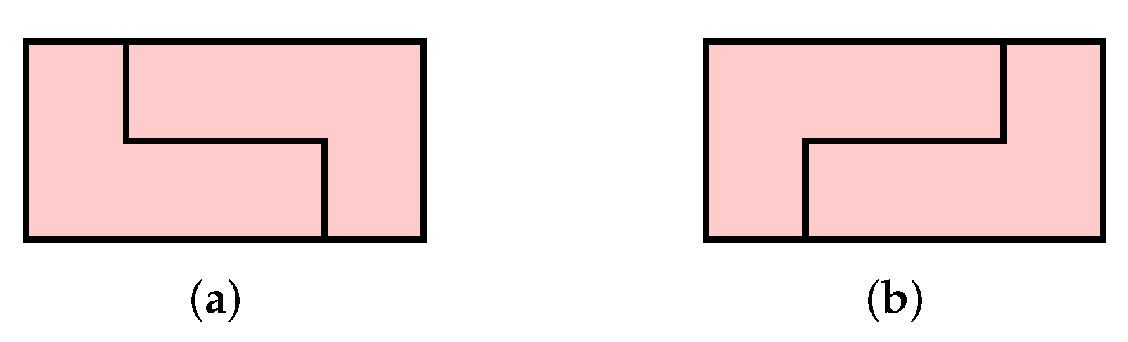
Consider the problem of tiling the rectangle, denoted R, with two L-shaped tetrominoes ![Algorithms 15 00164 i003]() , all orientations permitted. Initially, we review the basic ILP approach that was developed in [46] and then solve the same problem with the addition of colouring techniques.
, all orientations permitted. Initially, we review the basic ILP approach that was developed in [46] and then solve the same problem with the addition of colouring techniques.
 , all orientations permitted. Initially, we review the basic ILP approach that was developed in [46] and then solve the same problem with the addition of colouring techniques.
We introduce a variable for whether we use a particular placement of a tetromino ( coloured red) to tile the region, illustrated in Figure 1.
In any tiling of R, we must cover each of the eight cells exactly once, yielding the following system of eight linear equations in eight unknowns:
Observe that if we sum these equations, we obtain , which implies that we must use exactly two polyominoes to tile the region. Thus, this constraint is automatically incorporated into the system. A tiling of the region R corresponds to a binary solution of this system. However, solutions of the extended system where do not necessarily correspond to a tiling as solutions may also be rational. The reduced row echelon form of this system has seven non-zero rows and eight variables, thus one free variable. Solving this system, using a high-performance optimization package, such as CPLEX, Gurobi, or SCIP, yields two binary solutions: with all other variables equal to zero; and with all other variables equal to zero, illustrated in Figure 2. These tilings are trivial variations of each other, obtained by reflecting the entire board horizontally.
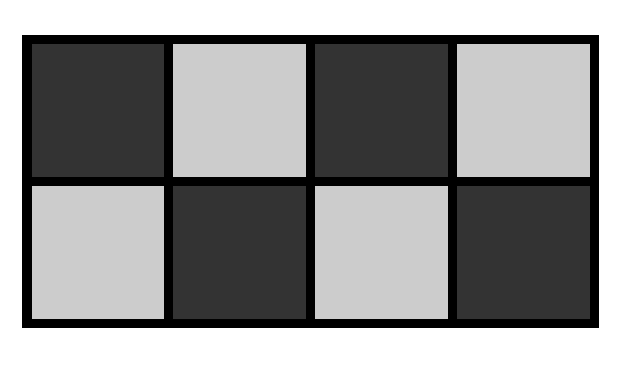
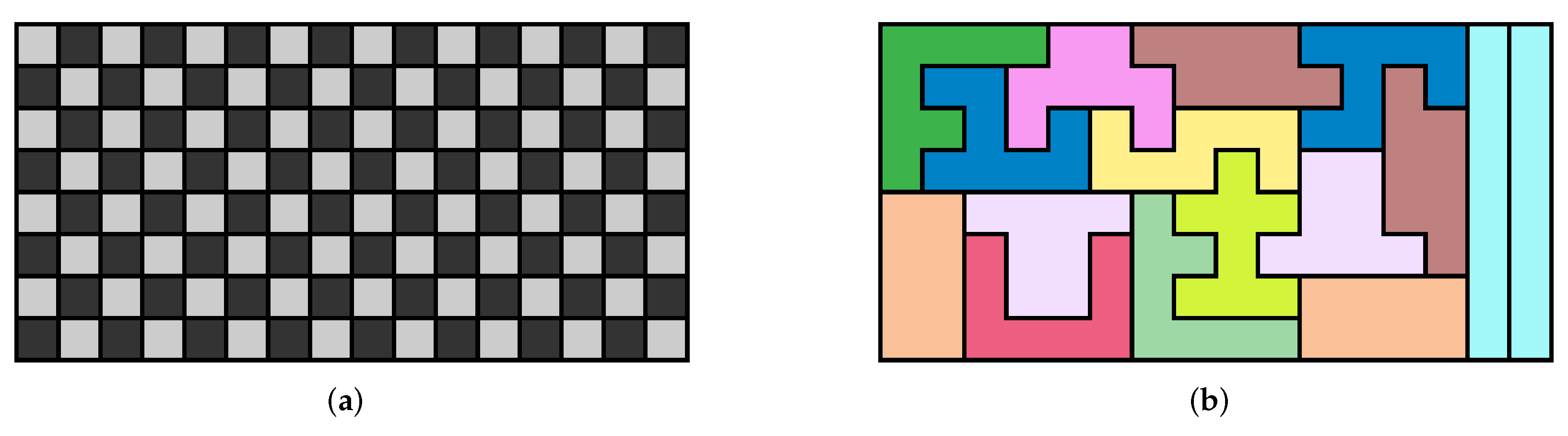
We now solve this tiling problem by including checkerboard colouring techniques. The starting point of the approach is to give the target region R a fixed checkerboard colouring, illustrated in Figure 3. There is another checkerboard colouring for this region obtained by swapping the black and white squares, but the particular choice of colouring does not matter to the solution procedure.
We also assume that the tetrominoes used to tile R have a checkerboard colouring, and the two distinct variants are
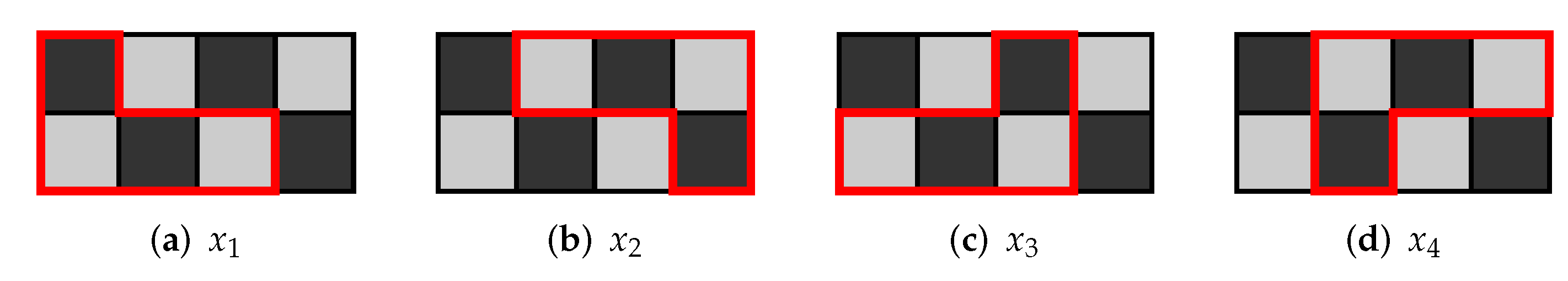
![Algorithms 15 00164 i004]() where all orientations are permitted. Not only must the coloured polyominoes fit in the target region, but the colouring of the cells covered must correspond to the colouring of the cells in the tiles. Using two coloured tetrominoes from this set yields three subcases: tiling with two of the first coloured tetromino; tiling with one coloured tetromino of each variant; or tiling with two of the second coloured tetromino. We focus on the first subcase. We introduce a variable for whether a particular placement of a coloured tetromino of the first kind in this set is used to tile the region, illustrated in Figure 4.
where all orientations are permitted. Not only must the coloured polyominoes fit in the target region, but the colouring of the cells covered must correspond to the colouring of the cells in the tiles. Using two coloured tetrominoes from this set yields three subcases: tiling with two of the first coloured tetromino; tiling with one coloured tetromino of each variant; or tiling with two of the second coloured tetromino. We focus on the first subcase. We introduce a variable for whether a particular placement of a coloured tetromino of the first kind in this set is used to tile the region, illustrated in Figure 4.
 where all orientations are permitted. Not only must the coloured polyominoes fit in the target region, but the colouring of the cells covered must correspond to the colouring of the cells in the tiles. Using two coloured tetrominoes from this set yields three subcases: tiling with two of the first coloured tetromino; tiling with one coloured tetromino of each variant; or tiling with two of the second coloured tetromino. We focus on the first subcase. We introduce a variable for whether a particular placement of a coloured tetromino of the first kind in this set is used to tile the region, illustrated in Figure 4.
In any tiling of the checkerboard coloured region in Figure 3, each of the eight cells must be covered exactly once, yielding the following system of eight linear equations in four unknowns:
If we sum these equations, we obtain , which again reflects the fact that we must use exactly two coloured polyominoes of the first variant to tile the region. Thus, this constraint is also automatically incorporated into the system. However, unlike in the previous example, this system has full rank and is thus trivially solved to yield with all other variables equal to zero, i.e., we have the first tiling solution illustrated in Figure 2. The third subcase is similar, yielding the second tiling solution illustrated in Figure 2.
In the second subcase, unlike the first and third subcases, we are tiling with two different coloured polyominoes. So each coloured polyomino has an associated constraint equation that must be incorporated into the linear system (i.e., unlike the case with a single polyomino or coloured polyomino, they are not both automatically incorporated into the linear system). This is like the multihedral case for tiling with polyominoes [46], which we review in the next section. The system of equations arising from the second subcase also has full rank; however, the unique solution of the extended system with is non-binary, and thus does not correspond to a tiling solution. This tiling example, although very simple, highlights an important point. When we combine checkerboard colouring techniques with the ILP approach for tiling, the problem can split into several subproblems with a reduction in subproblem complexity. Each subproblem is independently solvable, and the solutions to the full problem were partitioned among the subproblems.
The problem we introduced above is very simple, and not only because it is a small monohedral problem. The tetromino we used to tile the region is what we call ‘balanced’, i.e., when we apply a checkerboard colouring to this tile, the number of black cells is equal to the number of white cells. Thus, when tiling a region with N copies of a balanced tile, there will always be subcases to consider when seeking all tiling solutions: r tiles of the second coloured variant with tiles of the first coloured variant, where . However, we often tile with checkerboard coloured polyominoes that are not balanced, in which case the splitting of the full problem into subproblems depends on the ‘parity’ of the tiles and the target region, where we define parity as the number of black squares minus the number of white squares of a tile or region (see the next section and [47]).
1.2. Goals and Related Work
The traditional approach to tiling finite regions of the plane with polyominoes employs backtracking, which is the default way in computer science for exploring the search tree of a combinatorial problem [48,49,50,51,52]. Although backtracking is quick for some problems, it only refines a ‘brute-force’ solution procedure for exhaustively finding all solutions to a combinatorial search problem. Another less commonly used ‘brute-force’ approach to tiling with polyominoes employs either evolutionary computation [26] or genetic algorithms [53]; however, such approaches are likely considerably less efficient than backtracking. The only other general-purpose algorithmic procedure to tiling finite regions of the plane with polyominoes that we are aware of uses ILP, first introduced in [46]. There are several potential advantages of an algebraic approach to tiling over the backtracking methods. In [46], the authors note that with ILP the “the structure, combinatorial nature, and solvability of the model can be analyzed”. Finally, we mention there are many pure mathematical results for proving that a set of polyominoes tiles a region, for example, using the combinatorial group theory approach of J.H. Conway [54,55,56]. However, these methods typically apply only to special cases and thus, we cannot make them algorithmic.
It is interesting to note that the tiling problem, which is here regarded as an ILP instance, can also be considered a satisfiability problem (SAT) [57,58,59], for which there are a number of powerful solvers. Examples of suitable open-source SAT solvers include Lingeling; see http://fmv.jku.at/lingeling/ (accessed on 20 March 2022) and MapleSAT, see https://sites.google.com/a/gsd.uwaterloo.ca/maplesat/maplesat (accessed on 20 March 2022). Unfortunately, however, the overhead of enforcing the conditions that we use each tile a fixed number of times is prohibitive. Further details are provided in Appendix A.
The focus of the current article is to combine checkerboard colouring techniques adapted from [47] with a recently introduced ILP method [46] for tiling with polyominoes. The checkerboard colouring method [47] was originally used to identify large impossible tiling problems, i.e., the opposite of what we aim to do here. Our checkerboard colouring techniques often splits large tiling problems into smaller tiling subproblems, where each subproblem is represented as a separate ILP problem. Problems that are amenable to this approach are embarrassingly parallel. This article provides proof of concept of a parallelizable ILP approach for tiling finite regions of the plane with polyominoes. We construct the ILP formulations of the tiling problems in MATLAB and compute the numerical solutions using CPLEX, a high-performance optimization package. The primary goal is to analyze when this approach yields a potential parallel speedup.
For tiling problems solved via a parallelizable ILP optimization technique, there are two basic aims: (i) find a single tiling solution (i.e., an optimal solution), and (ii) find all tiling solutions. In the former case, when we apply our checkerboard colouring techniques, we seek the subcase yielding an optimal solution computed in the least amount of time. In the latter case, it is the subcase that takes the longest time to compute all solutions that is of interest; if this takes less time to compute than for the full (uncoloured) problem, then we have a potential parallel speedup.
The simple tiling examples discussed above raise many questions, namely the following:
- When do the checkerboard colouring techniques split the problem into multiple (≥2) independently solvable subproblems?
- For large problems (a large target region and/or the use of many tiles), what is an appropriate measure of problem complexity and the work done to compute tiling solutions?
- Under what situations does this ‘splitting’ technique yield a potential parallel speedup with parallel computing?
We structure the remaining parts of this article as follows. After giving some preliminary details about checkerboard colouring in Section 2, we describe how to build the ILP model formulation for tiling in Section 3. In Section 4, we describe how large tiling problems often split into many smaller tiling subproblems with the application of checkerboard colouring techniques. Section 5 deals with the theoretical issues of complexity, measures of performance, and problem classification. Section 6 presents the numerical solution of medium to large tiling problems, and in Section 7 we make some general comments about algorithm performance. Concluding remarks are in Section 8. Finally, in Appendix A, we discuss the possible application of an SAT solver to our tiling problem.
2. Preliminaries
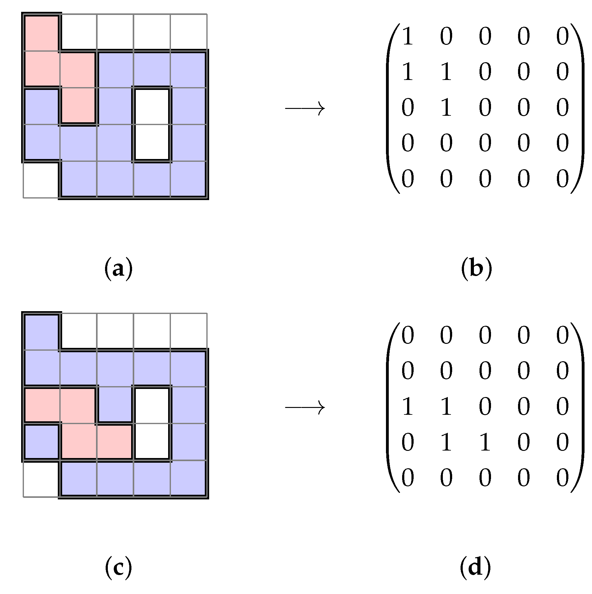
To begin our colouring approach to tiling, we give the target region R a checkerboard colouring, i.e., each black cell is only edge connected to white cells (and vice versa). We colour ‘white’ cells gray in all the figures of this article so that target regions with ‘holes’ stand out as white. We rigorously define a checkerboard colouring with the formula applied to position of each cell in the matrix representation of the region [60], where we identify the number with black cells and the number 0 with white cells. To reverse the colouring, we instead apply the formula . Polyominoes placed in a checkerboard coloured region acquire the colouring of the cells they cover. Changing the placement of a polyomino in R can reverse the colouring of a polyomino, i.e., black and white cells reverse.
The parity of a checkerboard coloured polyomino or region is the number of black cells minus the number of white cells [47]. When the number of black cells equals the number of white cells, the polyomino or region is balanced [31] (p. 17) and the parity is zero. If the parity of a polyomino or region R is non-zero, then there are two possible parity values denoted or respectively, where and p are positive integers. If the parity of a polyomino or region R is zero, then or , respectively.
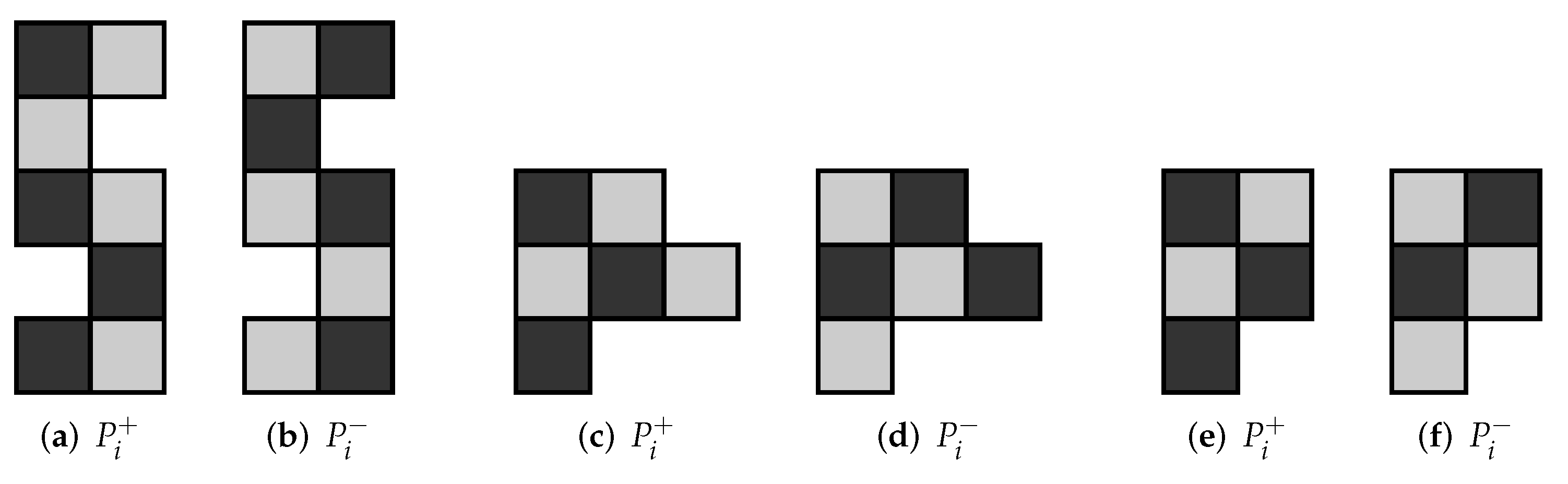
It is convenient to define a pariomino (pl. pariominoes) to be a particular checkerboard coloured polyomino. As the polyominoes are free, we also assume that the associated pariominoes are free. We denote the positive and negative parity pariominoes by and , respectively. Clearly, if we reverse the colouring of , we obtain (and vice versa). If the parity of a polyomino is zero, for notational convenience, we still represent the associated pariominoes by and , respectively. In the special case when the parity of a polyomino is zero and, then the particular choice of which variant we label and which is arbitrary (see Figure 5).
Depending on the symmetry of a polyomino , the number of possible orientations after applying rotations and reflections is 1, 2, 4, or 8. The associated pariomino will inherit the same number of possible orientations, except in the special situation when,
- (i)
- has 1, 2, or 4 orientations, and
- (ii)
- ,
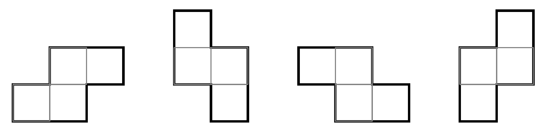
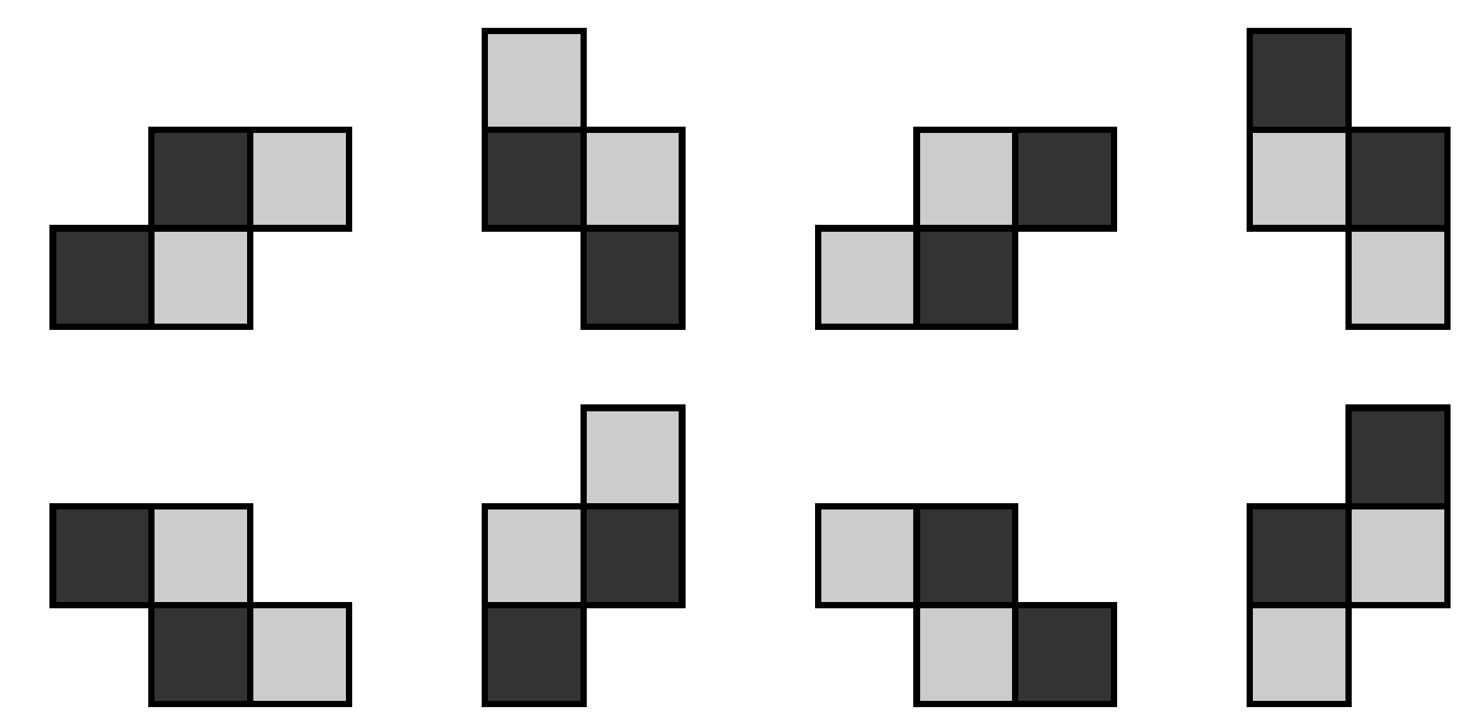
in which case we double the number of orientations. If , this implies that there exists a non-trivial rotation or a reflection that sends to (and vice-versa), which implies a balanced polyomino, i.e., the parity is zero. The converse statement is false, as there are many examples where the parity of a polyomino is zero, but the associated pariominoes are distinct (illustrated in Figure 5c,d). An example of a pariomino that has double the orientations of the corresponding polyomino is illustrated in Figure 6 and Figure 7. Each orientation of a polyomino or a pariomino represents a fixed polyomino or pariomino, respectively. We show below that the possible orientations of a polyomino or pariomino play a crucial role in developing our ILP colouring techniques for tiling.
3. ILP Model Formulation
In this section, we outline the ILP method for tiling. Initially, we construct binary matrices that are the key components of our models. Then, for the reader’s convenience, we review the derivation of the ILP formulations for the case of tiling with polyominoes [46] and then show how we adapt this approach to cover the case of tiling with pariominoes.
3.1. Construction of Binary Matrices
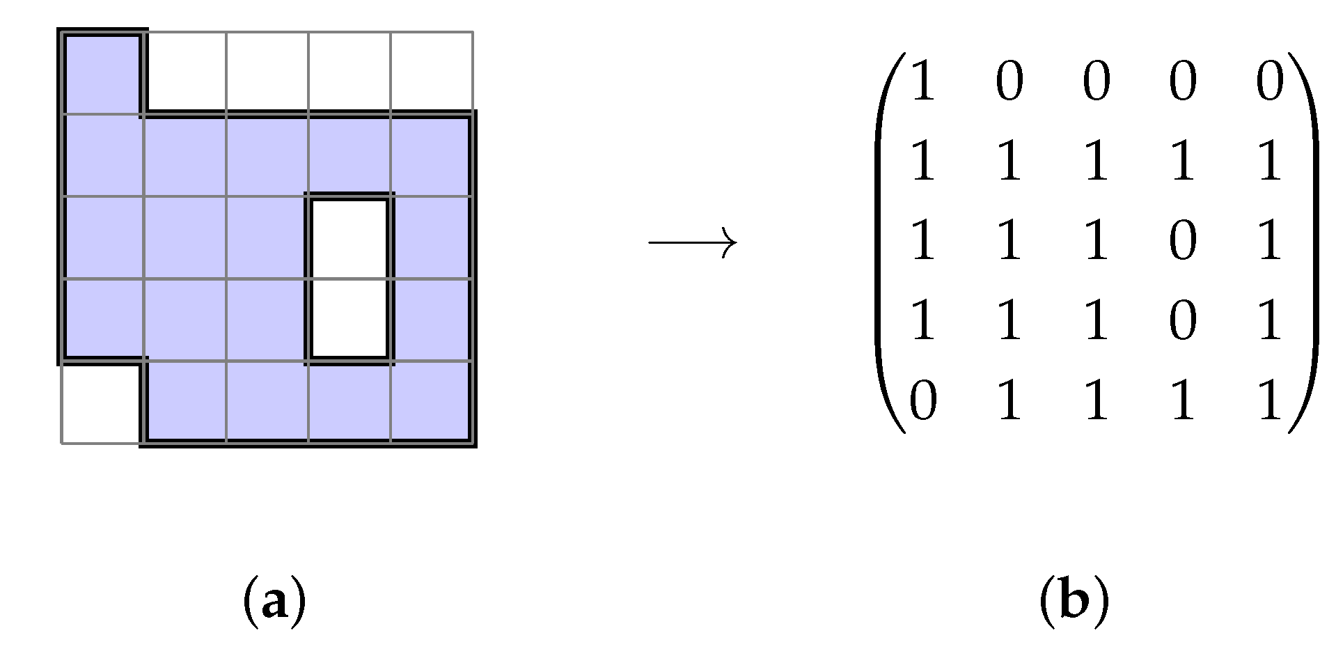
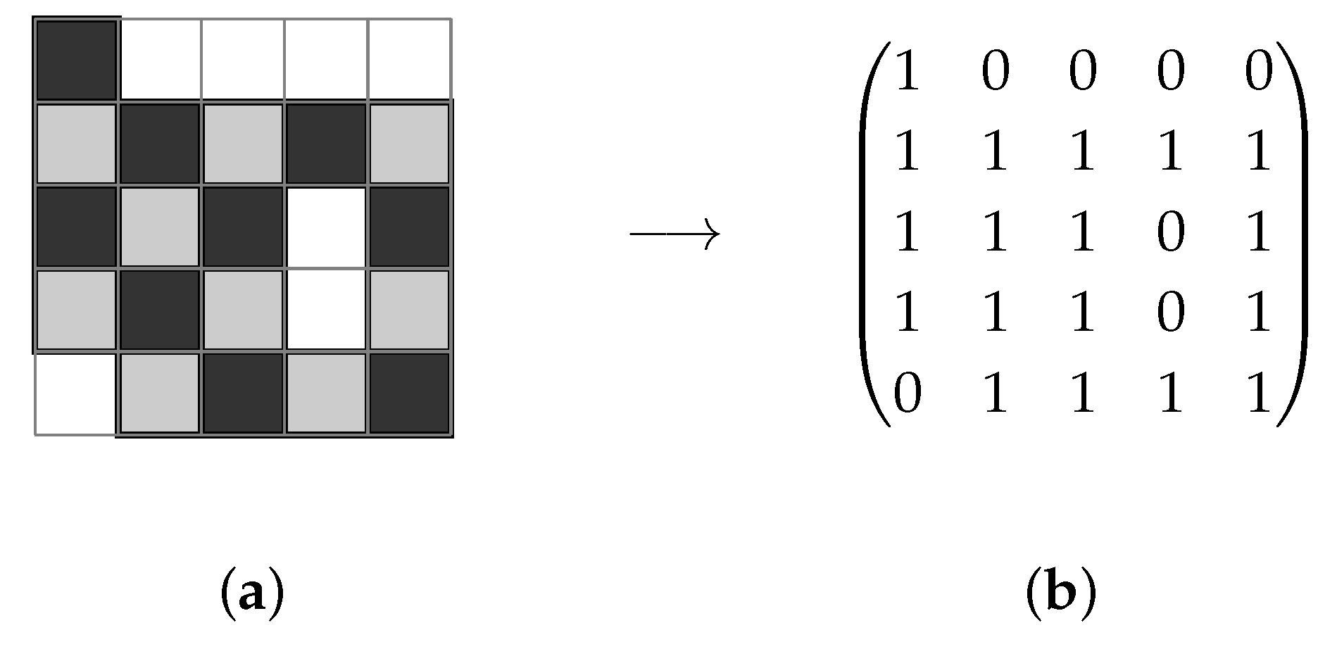
A key step in the ILP approach to tiling is to represent all placements of each polyomino in the target region R as binary matrices. The binary matrix associated with the j th placement of a polyomino in R is denoted . We also represent the target region R as a binary matrix denoted as B. The target region need not be rectangular and may have ‘holes’ and so, to represent it as a binary matrix, it is first positioned in the lattice of its rectangular hull. We illustrate an example in Figure 8 along with the associated binary matrix, where the th entry of B is equal to the number ‘1’ if there is a corresponding cell in the th position of R; otherwise, the th entry is equal to zero.
How we construct the binary matrices for each placement of a polyomino in R is similar. The -th entry of the binary matrix is equal to the number ‘1’ if there is a corresponding cell in the -th position of R covered by a cell of the polyomino; otherwise, the -th entry of is equal to zero. Figure 9 illustrates how we construct two binary matrices corresponding to different placements of a tetromino into R. Once we have constructed all the binary matrices, we assemble the ILP problem.
We must modify the procedure for constructing the binary matrices when fitting pariominoes into a checkerboard coloured region. Not only must the pariomino fit in the target region, but the colouring of cells covered must coincide with the colouring of cells in the pariomino, which generally yields a reduction in the total number of binary matrices compared to the polyomino tiling case. We construct the binary matrix B associated with a checkerboard coloured region in the same way as in the case without colouring. For example, Figure 10 illustrates how we construct B associated with a checkerboard colouring applied to the region in Figure 8. We obtain the same binary matrix if we reverse the checkerboard colouring of R, and the results of the checkerboard colouring approach in this work are independent of which colouring we use. Figure 11 illustrates the binary matrices associated with two different placements of the pariomino shown in Figure 7. To distinguish the pariominoes from the checkerboard coloured region containing them, we outline them in red. We denote the j-th placement of a pariomino or in a checkerboard coloured target region R by .
3.2. Assembly of the Linear Systems
For the reader’s convenience, we briefly review how to assemble the linear system of equations that makes up the ILP formulation of the polyomino tiling problem (see [46] for further details) and then discuss the modified procedure required when tiling with pariominoes.
Assume we wish to tile a target region R with area c using F free polyominoes with areas and the numbers of copies (). The total number of polyominoes used is . Clearly, the total area of R must equal the sum of the areas of the polyominoes, i.e., . Using a combination of rotations, reflections and translations, assume each polyomino fits ways into R. Recall the definitions of the binary matrices and B (see Section 3.1). We define Series i to be the set of all binary matrices associated with fitting the polyominoes into R, given by
The total number of binary matrices is given by , which also corresponds to the total number of possible placements of all polyominoes in the region R.
We introduce a variable , associated with , for whether the j-th placement of is used to tile R. The mathematical description of tiling the region R with copies of the F free polyominoes in is a natural one: we would like to know if there is a linear combination of the binary matrices , weighted by the respective that is equal to B. In this context, it is helpful to think of the binary matrix B as representing the fully tiled region R. The problem formulation is as follows.
Seek parameters , , such that
The constraints (4) enforce the conditions that we must use exactly polyominoes from each series i to tile R. It is easy to verify that the problem formulation automatically enforces the condition that the polyomino areas sum to the area of the target region.
It is a standard first-year university linear algebra exercise to convert matrix equations of the type (3) into a system of linear equations. After re-arranging the left-hand side of Equation (3) into a single matrix, we equate the non-zero entries of B with the corresponding entries in this matrix yielding c linear equations. The ordering of equations corresponds to reading entries in B left-to-right and top-to-bottom. Together with the constraints (4), this yields the following binary linear system of m equations in n unknowns:
Seek such that
The vertical lines in the solution vector separate the unknowns according to their corresponding series. Notice that the constraints (4) appear here as the -th equations, , namely (4), which just enforces the condition that exactly coefficients associated with each series k are equal to ‘1’, and the remaining coefficients are equal to zero. It is also helpful to note that if we neglect the rows in M corresponding to these constraints, then the columns of this ‘reduced’ coefficient matrix arise from the entries in the binary matrices written row-wise.
We claim that every problem, monohedral or multihedral, has one extraneous constraint equation because the main linear system corresponding to the first c equations essentially specifies the total number of squares covered. Once we impose all but one of the F constraint equations, we can work out the last constraint. We verify this by summing the first c equations in (5) to give
recalling that , and imposing the constraints (4). Hence, in the monohedral case, we do not have to include the single constraint in this formulation and so . However, for simplicity in our ILP formulations, we impose all the constraints in the multihedral case and exclude the single constraint in the monohedral case.
How we construct the linear system for the pariomino tiling problem is similar to the polyomino tiling problem, but with some important differences. Similar to the polyomino tiling problem, when we use multiple (≥2) free pariominoes to tile a region we refer to this problem as pari-multihedral; otherwise we refer to the pariomino tiling problem as pari-monohedral. We note it is possible for colouring techniques applied to a monohedral tiling problem to yield a pari-multihedral tiling problem. The notation we use for the linear system (5) still applies, but with some small changes. First, we denote the binary matrices instead of (see Section 3.1). Second, we denote the checkerboard coloured target region , to distinguish it from the uncoloured region R. Third, the number of free pariominoes used to tile , denoted , can differ from the number of free polyominoes F. This is because each polyomino with non-zero parity has two pariominoes associated with it, namely and , which are possibly distinct. Thus, generally we have . As in the polyomino tiling problem, the number of unknowns n is given by the total number of ways the distinct tiles (in this case, the pariominoes) fit into the target region . The number of equations m is also determined as in the polyomino tiling problem. In the pari-multihedral case, , while in the pari-monohedral case, .
The subtlety of the colouring approach relies on how we choose sets of pariominoes that split the full (uncoloured) problem into multiple independently solvable subproblems, covered in the next section.
4. A Splitting Method Using Parity Constraints
In [47], the authors used constraints on the parity values of the tiles to identify impossible tiling problems. We adapt these techniques here to split large tiling problems into many subproblems that admit a parallel solution strategy.
We attempt to tile a region R with parity p using F free polyominoes with copies , . Assume the polyominoes have parity values (if the parity value is zero then for ease of notation, we still represent the parity as ). Denote the multiset of all possible sums of parity values by , , namely, all possible sums of
where and , for .
It is easy to prove the combinatorial result that [47]:
Proposition 1.
The number of sums of parity values that we can form from (6) is
The following simple result is key to the arguments that follow [47]:
Proposition 2.
A necessary (but not sufficient) condition for the polyominoes to tile a region R is that for at least one .
When none of the possible parity sums equals the parity of the target region, we call this a parity violation, which implies that it is impossible for the given polyominoes to tile the target region. In this work, we are more interested when we know ahead of time that the polyominoes do tile the target region R, in which case many combinations of parity values may satisfy Proposition 2. Each solution satisfying Proposition 2 corresponds to a separate tiling subproblem with pariominoes that may or may not tile . The total number of possible tiling solutions is partitioned among all the pariomino tiling subproblems.
It is possible to compute all solutions satisfying Proposition 2 using brute-force techniques. However, this rapidly becomes intractable for large problems. The decision problem of whether there is a solution that satisfies Proposition 2 is related to the general subset sum problem, which is -complete [61]. For this reason, we apply a systematic mathematical procedure for solving this problem using linear Diophantine equations. We adapt the arguments given below from [47].
If all F polyominoes have zero parity, then we must have so Proposition 2 is trivially satisfied. Now consider the case that at least one polyomino has non-zero parity. Assume, without loss of generality, the first r polyominoes, have zero parity. Let the variable denote how many of the non-negative elements drawn from are , , . We derive an equation in the variables that matches the sum of the parities of the tiles to the parity of the target region. As we have choices for how many of the elements drawn from are , we must have choices of , , . Then the equation takes the form
or after some simplification
for , which is a linear Diophantine equation in unknowns . We can easily verify that it is safe to divide both sides by 2, yielding the following.
Theorem 1.
The number of distinct solutions satisfying Proposition 2 is given by the number of solutions of the following linear Diophantine equation in unknowns :
A necessary condition for the existence of integer solutions (and hence also for non-negative integer solutions) of Equation (7) is , where denotes the greatest common divisor of [62] (p. 30). When we know there is a solution to the full (uncoloured) tiling problem, then this condition is automatically satisfied. Suppose a solution exists. Consider an arbitrary polyomino . Notice that if or , then we tile the coloured region R with copies of the pariomino or respectively. That is, there is a single pariomino associated with in the pariomino tiling problem. On the other hand, if and , then we use copies of and copies of in the pariomino tiling problem, i.e., we use both and . Thus, the relationship between the number of free polyominoes F and the associated number of free pariominoes is given by
As each solution satisfying Proposition 2 yields a separate pariomino tiling subproblem, Theorem 1 yields a practical means of splitting the full (uncoloured) tiling problem into separate subproblems that are independently solvable. Furthermore, the full set of solutions is partitioned among the solutions of the subproblems, and thus, the problem of finding all solutions is embarrassingly parallel.
As we saw from the simple example outlined in the introduction, there is another mechanism that splits a tiling problem into subproblems, separate from those identified using Theorem 1. If some parities are zero with , then more subproblems exist, as each polyomino of this type yields two choices for the pariominoes, multiplying the number of subproblems by a factor of two in each instance.
For simplicity, assume for a tiling problem that none of the polyominoes satisfies and , i.e., we exclude the alternate ‘splitting’ mechanism described above. Then Algorithm 1 gives a simple procedure for finding all tiling solutions (the algorithm is easily modified to account for the alternate ‘splitting’ mechanism if required). Our starting point is a target region R with area c and parity p, which we aim to tile using polyominoes with areas and copies , . As stated earlier, we assume the parities are zero (). We also assume that the tiling problem has at least one solution.
| Algorithm 1 To find all possible solutions of a polyomino tiling problem using checkerboard colouring arguments and ILP |
|
A small modification of Algorithm 1 yields an algorithm for computing a single solution to one of the pariomino subproblems in the least amount of time. In line 10, instead of calculating all solutions for each subproblem, we seek a single optimal solution and break the ‘parallel-for-loop’ as soon as soon as we find the first optimal solution.
5. Some Theoretical Considerations
In this section, we consider the related concepts of problem complexity; measures of algorithm performance; and problem classification. Before discussing the results from the numerical examples of Section 6, we make some general comments that relate to the questions raised in the introduction.
5.1. Complexity
One way to estimate the complexity of a problem is to measure the computational work required to solve it. We can also use complexity to compare the difficulty of two problems or the effectiveness of two algorithms. For the tiling problem, some factors that might form a complexity measure on theoretical grounds include the number of unknowns, the number of constraints, and the number of free variables of the associated ILP problem.
Recall that the number of binary matrices for a tiling problem yields the number of unknowns in the resulting linear system. When we apply checkerboard colouring techniques, if we use every pariomino and , for , the number of unknowns in the linear systems for the pariomino and polyomino tiling problems are the same. However, for each polyomino when the corresponding pariomino used to tile R is or (but not both), then the number of binary matrices (and hence the number of unknowns) in the linear system for the pariomino tiling problem is usually reduced, compared to the corresponding polyomino tiling problem. However, it is possible to construct some problems where this is not the case (see Section 6.2).
It is also worth considering in the multihedral case the role played by the number of constraints on the problem complexity. Each polyomino or pariomino contributes a constraint to the associated linear systems. Assuming the ILP problem is feasible, then it is reasonable to assume from a computational perspective that the more constraints we have the better. This is because the linear systems are usually underdetermined, and so it is helpful if the augmented matrix is as close to full rank as possible. As we often have we expect the rank of the augmented matrix for many pariomino tiling problems to be closer to the full rank than the augmented matrix for the polyomino tiling problem (even when the number of unknowns in the two systems is the same).
Thus to summarize, it is reasonable when we consider both the number of unknowns and the number of constraints in an ILP problem, that in general, we see an improvement in the solvability of a pariomino tiling subproblem compared to the solvability of the full (uncoloured) tiling problem. However, because of the complexity of the general tiling situation, we cannot prove the superiority either algorithmically or theoretically.
After many experiments, none of these measures seem to provide a reliable work estimate when judged by the time it takes an ILP solver to handle the problem. This may in part be because the ILP solver has a variety of techniques available and there are many features of a problem hidden from our analysis, which makes a simple complexity formula impossible. The possibly hidden structure in an ILP problem either hinders or helps the ILP solver to find solutions [63,64]. Without a complexity formula based on theoretical grounds, we use the runtime of a fixed computer system. In our experience, this produces a reliable, repeatable, and practical substitute for a complexity formula. Although runtimes differ depending on the computer architecture and even the software version, it allows us to make practical comparisons between different tiling problems, or between subproblems of the same tiling problem.
5.2. Measures of Performance
With the runtime as our basic measure of computational work, we also need an appropriate measure of improvements in runtime obtained using our checkerboard colouring technique. In parallel computing, the speedup of an algorithm for solving a given problem with a fixed number of processors is given by [65]
As this article provides only proof of concept of a parallel implementation, in place of speedup for finding all tiling solutions of a problem, we define the potential speedup for a tiling problem to be
When seeking a single optimal solution, we define the potential speedup as
5.3. Problem Classification
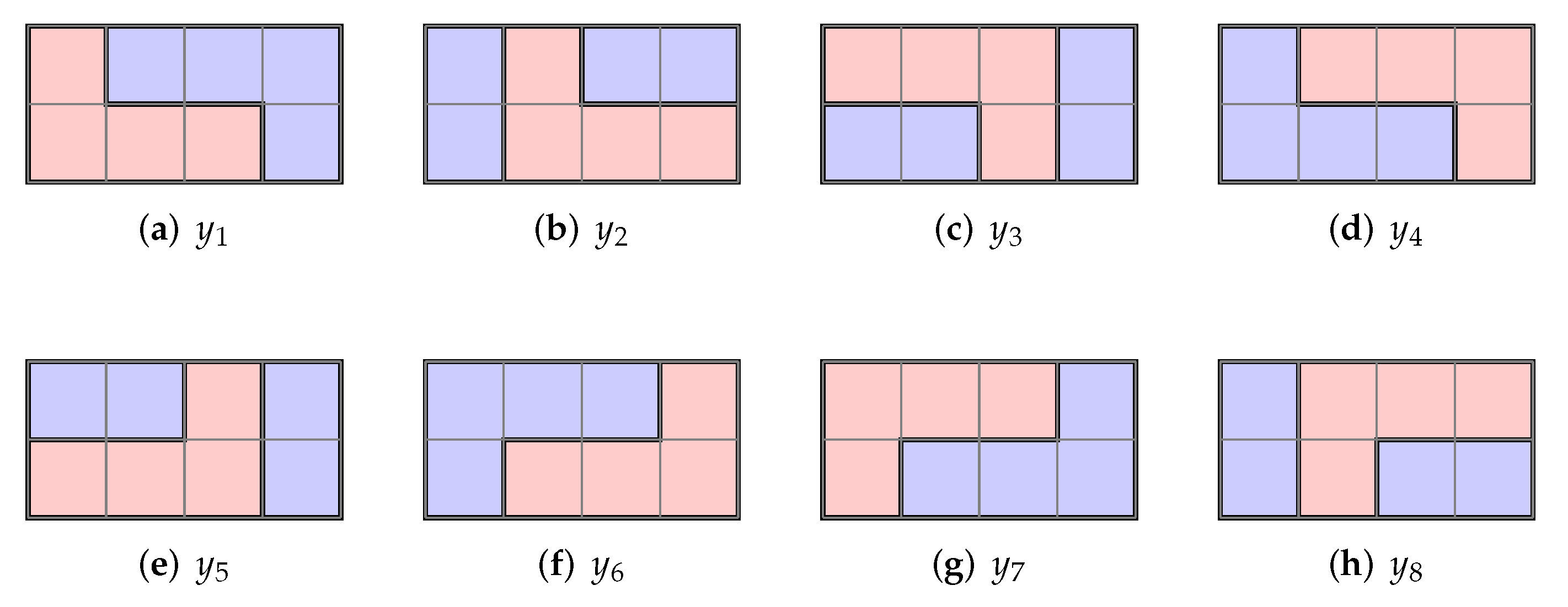
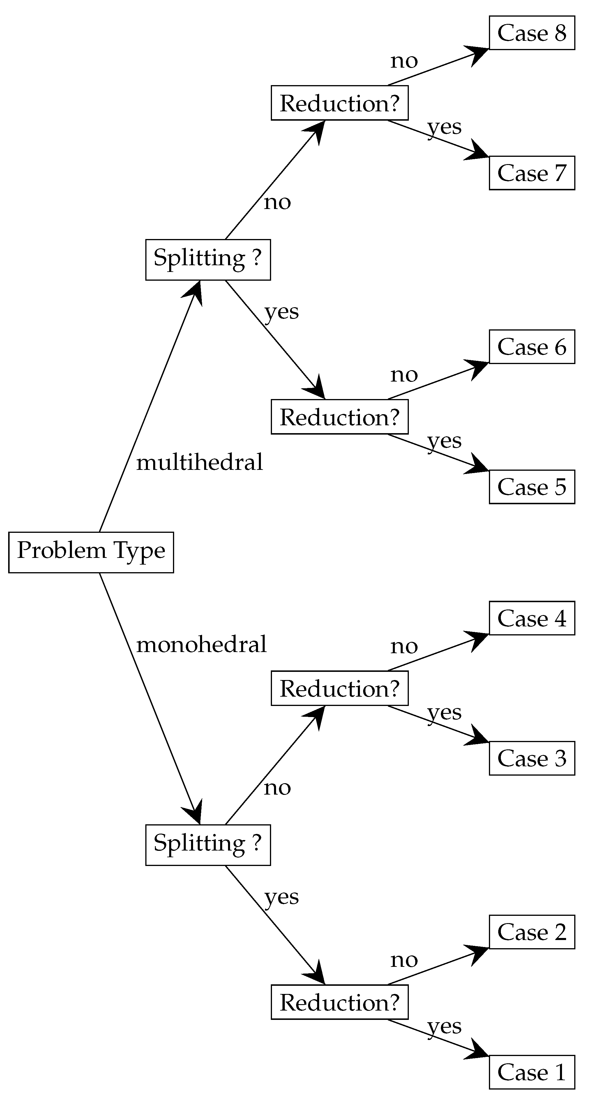
We classify the different situations arising when we apply checkerboard colouring arguments to a polyomino tiling problem. Either we have a monohedral polyomino tiling problem, or a multihedral polyomino tiling problem. For these two types of problems, the full tiling problem either splits into multiple pariomino tiling subproblems, or it does not (i.e., there is a single pariomino tiling problem to consider). In each of these four situations, the resulting pariomino tiling problems may or may not yield a reduction in complexity (compared to the full uncoloured tiling problem), yielding the eight cases illustrated in Figure 12.
6. Numerical Examples
We solve many tiling problems, either for all solutions, or a single (optimal) solution, using appropriate software.
We introduce some notation that helps us refer to the number of pariomino variants used in each tiling problem. Recall when we have copies of a pariomino with positive parity, then we have copies of a pariomino with negative parity. For notational convenience in this section, we define , so , for . We must be a little careful with our notation when the parity of a polyomino is zero (recall, in this situation for notational convenience, we still refer to the and variants). If and we allow ourselves a slight abuse of notation by still using to represent the number of variants and to represent the number of variants. However, we cannot use this notation when (and so ) as in this case, the number of copies used is always .
6.1. Scientific Computing
We solved all tiling problems using MATLAB (R2020b) and CPLEX (12.8.0.0), a commercial optimization package, see https://www.ibm.com/analytics/cplex-optimizer (accessed on 20 March 2022), run on a MacBook Pro (OS X 10.15.7) with 16 GB memory and 2.7 GHz Intel Core i7. In a previous study [46] we verified that CPLEX was very effective at solving the ILP problems arising from tiling with polyominoes, and was generally faster than two other popular high-performance optimization packages, namely Gurobi (7.5.2), see http://www.gurobi.com (accessed on 20 March 2022), and SCIP (6.0.0), see http://scip.zib.de (accessed on 20 March 2022). The shell commands needed in CPLEX to find either all feasible solutions, or a single optimal solution, are given in [46].
To solve a particular instance of a tiling problem we employed three steps:
- (i)
- Construct the linear system in MATLAB and export the associated ILP file to CPLEX;
- (ii)
- Solve the ILP file with CPLEX and export the solution file back to MATLAB;
- (iii)
- Extract the solution(s) from the file produced in (ii) in a form that MATLAB can read and plot.
We provide all necessary files for other researchers to reproduce the experimental results in this article. The collections of MATLAB files needed to carry out steps (i) and (iii) above for the polyomino and pariomino tiling problems are freely available. The associated repositories are POLYOMINOES (v2.1.4), see https://0-doi-org.brum.beds.ac.uk/10.5281/zenodo.6366101 (accessed on 20 March 2022), and PARIOMINOES (v3.0.0), see https://0-doi-org.brum.beds.ac.uk/10.5281/zenodo.6366094 (accessed on 20 March 2022). For every example, we provide the appropriate MATLAB ‘LP make’ files. In the polyomino tiling case, solutions are plotted in MATLAB using the programs PLOT_MONO or PLOT_MULTI, depending on whether the problem is of the monohedral or multihedral type, respectively. In the pariomino tiling case, solutions are plotted in MATLAB using the program PLOT_PARIOMINO. The MATLAB program DIOPHANTINE_ND_NONNEGATIVE_BOUNDED, included in the PARIOMINOES repository, was used to solve the linear Diophantine Equations (7) of Theorem 1. This program is similar in construction to the related Diophantine solvers described at [47].
From a computational perspective, it would simplify the solution process if we could encode the parity constraints of Equation (7) directly into the ILP formulation. However, before the ILP formulation can be constructed we must first solve (7) yielding sets of pariominoes, where each set represents a separate pariomino tiling subproblem. Then, for each subproblem, the MATLAB programs in the repository PARIOMINOES are used to construct an ILP file. This is a non-trivial task because before we can compute the constraints we must compute all possible placements of the pariominoes in the checkerboard coloured target region. In addition to fitting the pariominoes in the region (using a combination of rotations, reflections and translations) we also ensure that the colours of squares covered match the colours of the squares of the tiles (see Section 3 for further details).
6.2. Tiling Examples Where All Solutions Are Sought
We give tiling examples for seven out of the eight cases illustrated in Figure 12. In all examples, we compare the solution process with and without using checkerboard colouring techniques. In the ILP context, we use a zero objective function and refer to the m linear equations in the resulting binary linear systems as constraints. The number of free variables f relates to the reduced row echelon form of the augmented systems . When we apply colouring techniques, we say the full (uncoloured) tiling problem yields a ‘splitting’ if there are two or more associated pariomino tiling subproblems. We say there is a ‘reduction in complexity’ if the maximum CPLEX runtime for all pariomino tiling subproblems is less than the runtime required to solve the full (uncoloured) tiling problem, i.e., the potential speedup is greater than 1 (see Section 5.2). As a check of the correctness of our results, in each example, we checked that the total number of solutions found after solving all subproblems equaled the total number of solutions found for the uncoloured tiling problem.
According to our classification system, monohedral tiling problems naturally fall into one category on the tree in Figure 12. However, in contrast to the multihedral case, it was not always possible to find completely satisfactory representatives for each case of the monohedral tiling problems. Some cases of questionable significance yielded a small reduction in computational time. Other contrived cases, which were found with a satisfactory reduction in computational time, are not typical. Thus, some of the monohedral examples labeled with an asterisk (*) indicate that their exact placement in our classification tree is questionable.
6.2.1. Case 1
We give an example of the monohedral polyomino type, where applying colouring techniques splits the full (uncoloured) polyomino tiling problem into multiple pariomino tiling subproblems, with a reduction in complexity.
Example 1.
![Algorithms 15 00164 g013]()
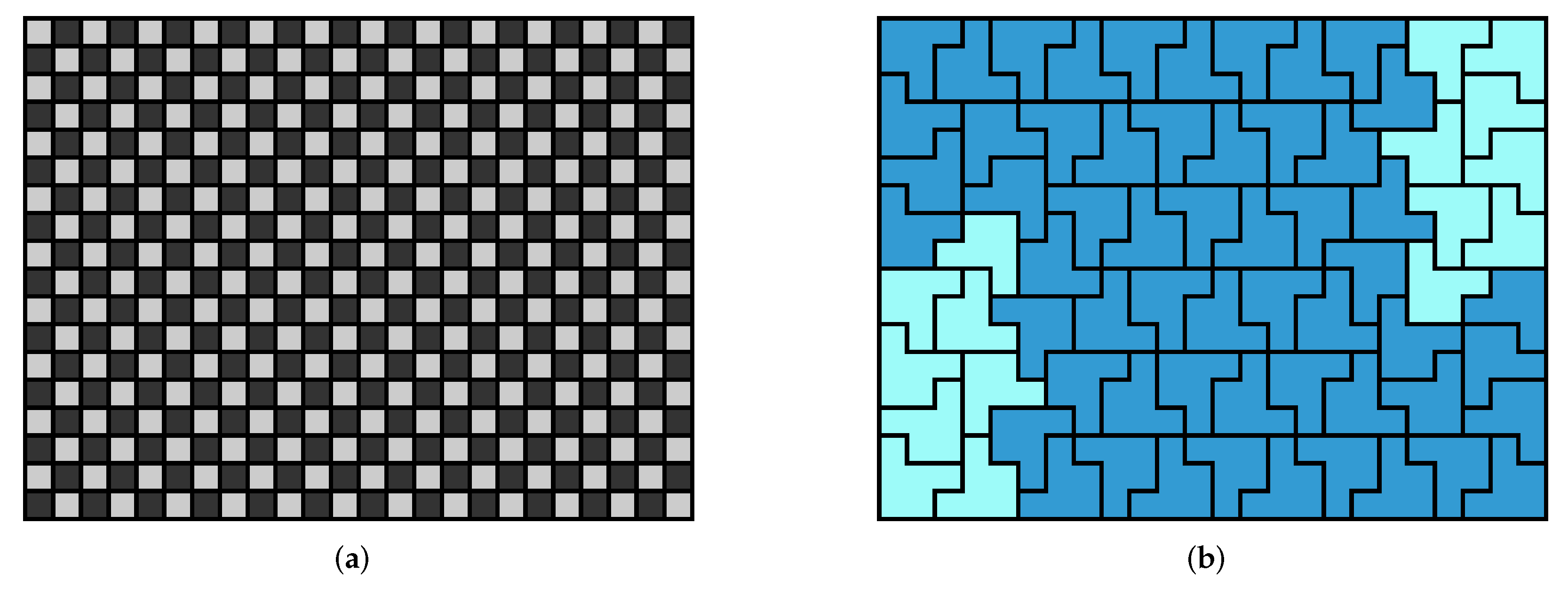
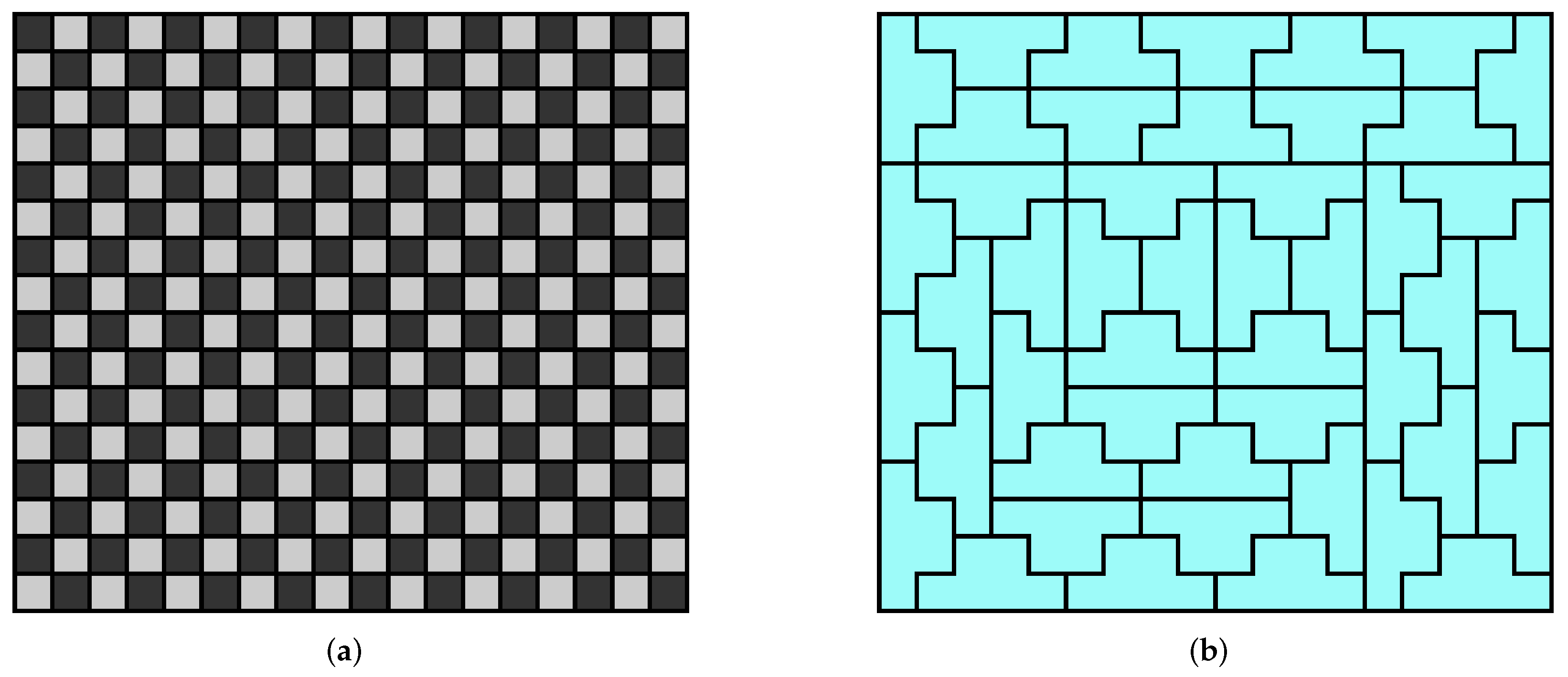
Find all ways of tiling the 9-by-9 single-notched square![Algorithms 15 00164 i005]() all orientations permitted. The area of R is 80, so we need 20 copies of the L-shaped tetromino. The associated binary ILP file, constructed with the program LPMAKE_POLYOMINOES_FIGURE2, has n = 442 unknowns, m = 80 constraints, and f = 363 free variables. CPLEX
found 1,709,594 solutions in 367.9 s.
all orientations permitted. The area of R is 80, so we need 20 copies of the L-shaped tetromino. The associated binary ILP file, constructed with the program LPMAKE_POLYOMINOES_FIGURE2, has n = 442 unknowns, m = 80 constraints, and f = 363 free variables. CPLEX
found 1,709,594 solutions in 367.9 s.
 all orientations permitted. The area of R is 80, so we need 20 copies of the L-shaped tetromino. The associated binary ILP file, constructed with the program LPMAKE_POLYOMINOES_FIGURE2, has n = 442 unknowns, m = 80 constraints, and f = 363 free variables. CPLEX
found 1,709,594 solutions in 367.9 s.
all orientations permitted. The area of R is 80, so we need 20 copies of the L-shaped tetromino. The associated binary ILP file, constructed with the program LPMAKE_POLYOMINOES_FIGURE2, has n = 442 unknowns, m = 80 constraints, and f = 363 free variables. CPLEX
found 1,709,594 solutions in 367.9 s.Using colouring techniques we wish to tile the checkerboard coloured regionshown in Figure 13a using 20 pariominoes from the set![Algorithms 15 00164 i006]() all orientations permitted.
all orientations permitted.
 all orientations permitted.
Table 1.
Number of tiling solutions (# solns.) and runtimes in seconds for CPLEX to find the feasible solutions of the pariomino tiling problem in Example 1.
Table 1.
Number of tiling solutions (# solns.) and runtimes in seconds for CPLEX to find the feasible solutions of the pariomino tiling problem in Example 1.
| 20 | 18 | 16 | 14 | 12 | 10 | 8 | 6 | 4 | |
| 0 | 2 | 4 | 6 | 8 | 10 | 12 | 14 | 16 | |
| # solns. | 406 | 9762 | 72,308 | 252,844 | 475,908 | 503,612 | 296,004 | 88,498 | 10,212 |
| runtime (s) | 0.09 | 2.16 | 16.30 | 72.49 | 121.67 | 138.52 | 83.01 | 28.88 | 3.15 |
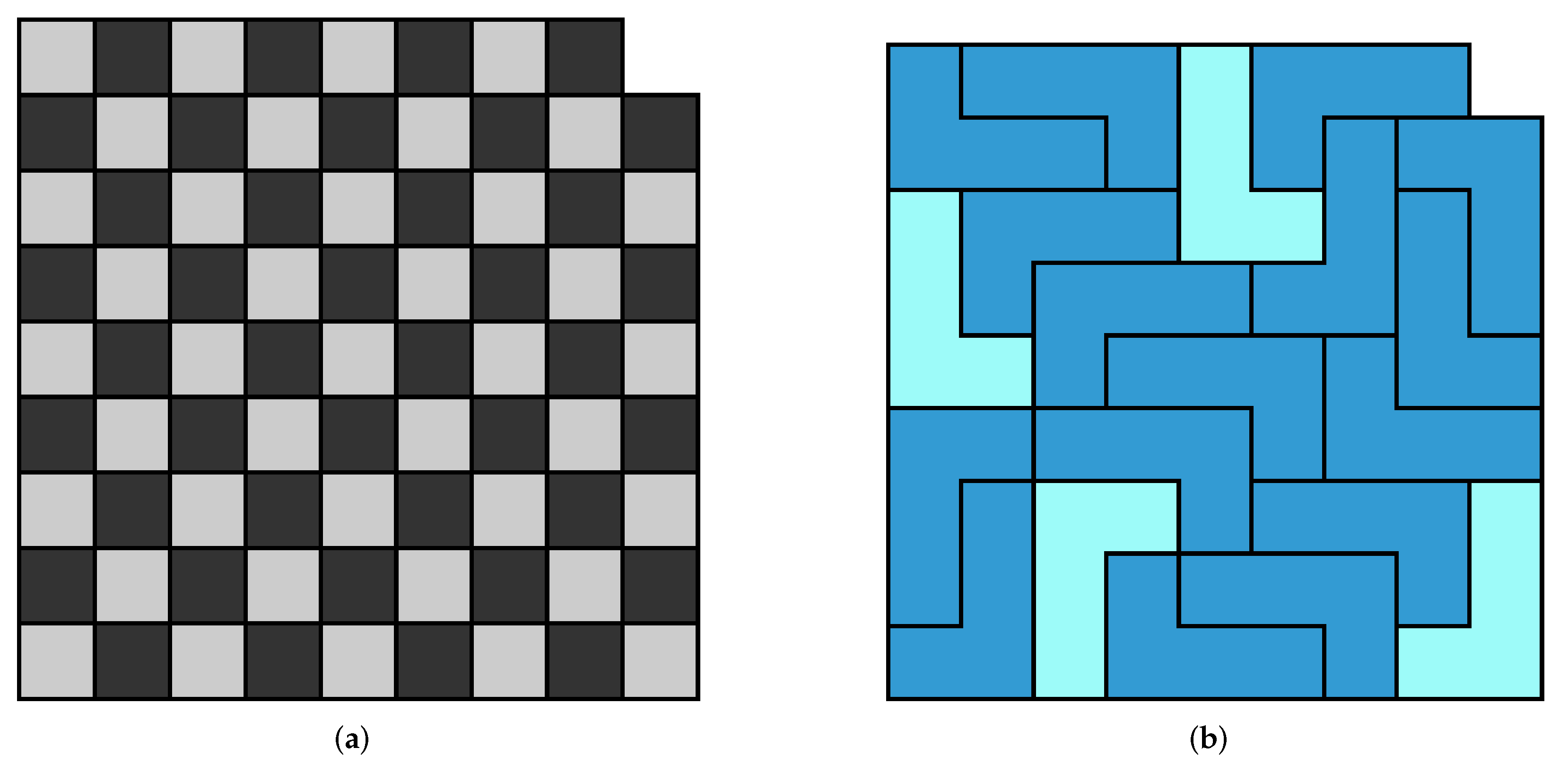
Figure 13.
Target region and a tiling solution for Example 1: (a) The target region , a checkerboard coloured 9-by-9 single-notched square; (b) Successful tiling of the target region using 20 copies of an L-shaped tetromino. The variants are coloured light-blue and the variants coloured dark-blue corresponding to an optimal solution of the subproblem with (see Table 1).

As the tetromino and R have zero parity and we automatically obtain 21 tiling subproblems to consider with and copies of and respectively, given by for . Solving the subproblems in CPLEX yielded the data for the nine feasible solutions shown in Table 1, where we report the number of solutions found (# solns.), and the runtime (in seconds).
A single (optimal) tiling solution corresponding to the subproblem with is shown in Figure 13b, i.e., using four copies of and 16 copies of . The ILP file in this case was constructed using the program LPMAKE_PARIOMINOES_FIGURE2 (similar programs were used to construct the ILP files for the other cases). The subproblems with either and , or and , yielded and respectively. All other subproblems yielded . The maximum runtime for the infeasible solutions was 0.62 s. The subproblem with the maximum runtime of s yielded 503,612 solutions, thus the potential speedup when using the colouring technique is about 2.7×.
6.2.2. Case 2
We give two examples of the monohedral polyomino type, where the application of colouring techniques splits the full (uncoloured) polyomino tiling problem into multiple pariomino tiling subproblems, with no reduction in complexity.
Example 2 (*).
Find all ways of tiling the 18 × 24 rectangle with![Algorithms 15 00164 i007]() all orientations permitted. The area of R is 432, so we need 72 copies of the hexomino. The associated ILP file, constructed with the program LPMAKE_POLYOMINOES_FIGURE3, has n = 2816 unknowns, m = 432 constraints, and f = 2385 free variables. CPLEX found 414 solutions in s.
all orientations permitted. The area of R is 432, so we need 72 copies of the hexomino. The associated ILP file, constructed with the program LPMAKE_POLYOMINOES_FIGURE3, has n = 2816 unknowns, m = 432 constraints, and f = 2385 free variables. CPLEX found 414 solutions in s.
 all orientations permitted. The area of R is 432, so we need 72 copies of the hexomino. The associated ILP file, constructed with the program LPMAKE_POLYOMINOES_FIGURE3, has n = 2816 unknowns, m = 432 constraints, and f = 2385 free variables. CPLEX found 414 solutions in s.
Using colouring techniques, we wish to tile the checkerboard coloured region shown in Figure 14a using 72 pariominoes from the set![Algorithms 15 00164 i008]() all orientations permitted.
all orientations permitted.
 all orientations permitted.
As the hexomino and R have zero parity and we automatically obtain 73 tiling subproblems to consider with and copies of and respectively, given by for . Solving the subproblems in CPLEX
yielded the data for the 23 feasible solutions shown in Table 2.
A single (optimal) tiling solution corresponding to the subproblem with is shown in Figure 14b. The program LPMAKE_PARIOMINOES_FIGURE3 was used to construct the ILP file in this case. (Similar programs were used to construct the ILP files for the other cases.) The subproblems with either and , or and , yielded . All other subproblems yielded . The maximum runtime for the infeasible solutions was 6.3 s. The subproblem with the maximum runtime of 15.30 s yielded 94 solutions, which is an increase in the runtime of approximately 7.60% compared to the full (uncoloured) tiling problem, i.e., no potential speedup was observed.
Table 2.
Number of tiling solutions (# solns.) and runtimes in seconds for CPLEX to find the feasible solutions of the pariomino tiling problem in Example 2.
Table 2.
Number of tiling solutions (# solns.) and runtimes in seconds for CPLEX to find the feasible solutions of the pariomino tiling problem in Example 2.
| 16 | 26 | 27 | 28 | 29 | 30 | 31 | 32 | 33 | 34 | 35 | 36 | |
| 56 | 46 | 45 | 44 | 43 | 42 | 41 | 40 | 39 | 38 | 37 | 36 | |
| # solns. | 1 | 4 | 2 | 4 | 6 | 9 | 12 | 31 | 26 | 51 | 14 | 94 |
| runtime (s) | 2.2 | 8.7 | 8.5 | 10.2 | 8.8 | 10.1 | 9.8 | 13.3 | 9.6 | 11.0 | 9.9 | 15.3 |
| 37 | 38 | 39 | 40 | 41 | 42 | 43 | 44 | 45 | 46 | 56 | - | |
| 35 | 34 | 33 | 32 | 31 | 30 | 29 | 28 | 27 | 26 | 16 | - | |
| # solns. | 14 | 51 | 26 | 31 | 12 | 9 | 6 | 4 | 2 | 4 | 1 | - |
| runtime (s) | 12.8 | 12.6 | 10.6 | 12.6 | 12 | 10.7 | 8 | 8.8 | 7.6 | 8.1 | 3.7 | - |
Figure 14.
Target region and a tiling solution for Example 2: (a) the target region , a checkerboard coloured rectangle; (b) successful tiling of the target region using 72 copies of a hexomino. The variants are coloured light-blue and the variants coloured dark-blue corresponding to the optimal solution of the subproblem with (see Table 2).

Example 3 (*).
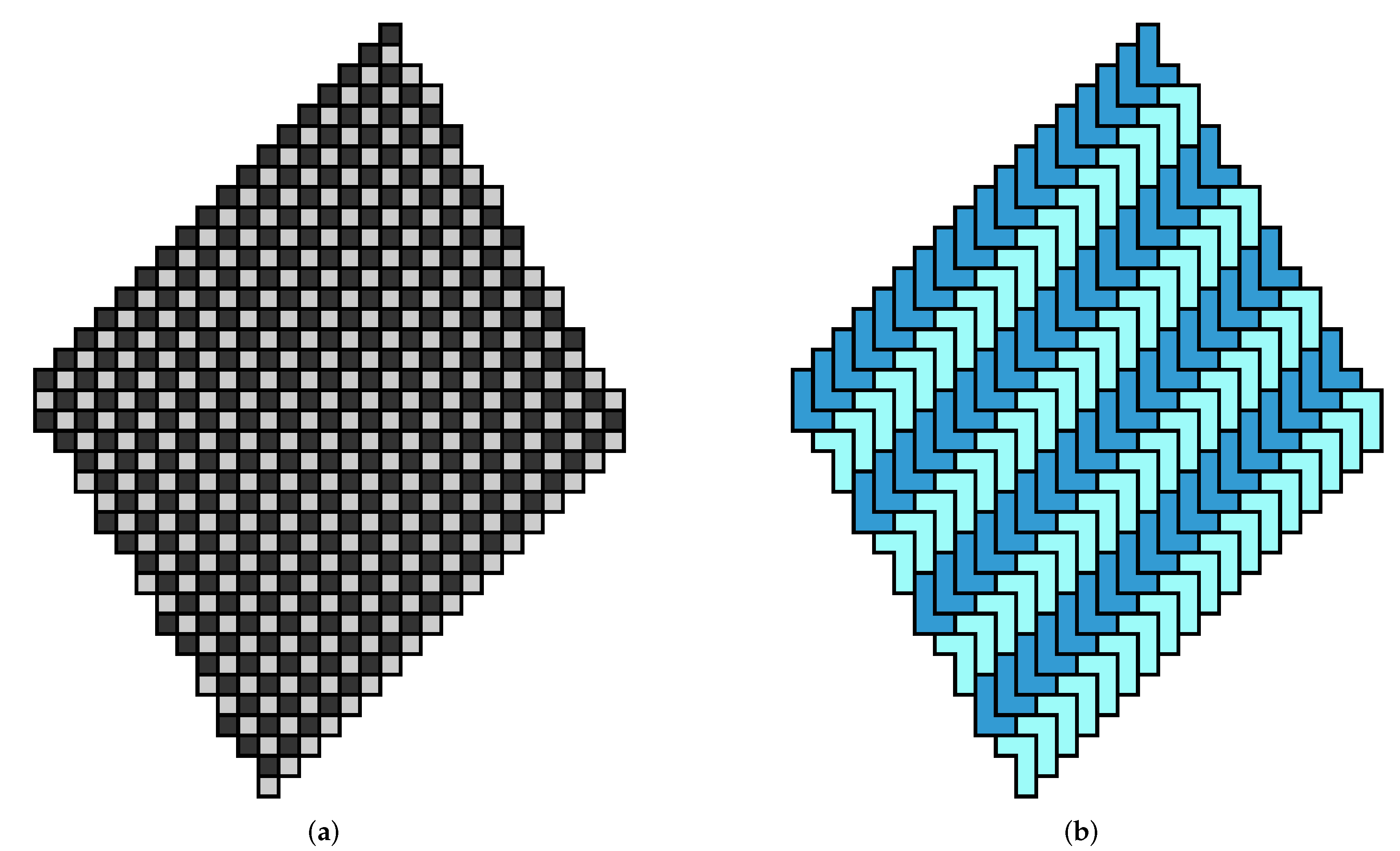
Find all ways of tiling the irregularly shaped region![Algorithms 15 00164 i009]() all orientations permitted. The area of R is 576, so we need 144 copies of the L-shaped tetromino. The associated ILP file, constructed with the program LPMAKE_POLYOMINOES_FIGURE4, has n = 3952 unknowns, m = 576 constraints, and f = 3377 free variables. CPLEX found a single solution in 0.15 s.
all orientations permitted. The area of R is 576, so we need 144 copies of the L-shaped tetromino. The associated ILP file, constructed with the program LPMAKE_POLYOMINOES_FIGURE4, has n = 3952 unknowns, m = 576 constraints, and f = 3377 free variables. CPLEX found a single solution in 0.15 s.
 all orientations permitted. The area of R is 576, so we need 144 copies of the L-shaped tetromino. The associated ILP file, constructed with the program LPMAKE_POLYOMINOES_FIGURE4, has n = 3952 unknowns, m = 576 constraints, and f = 3377 free variables. CPLEX found a single solution in 0.15 s.
Using colouring techniques we wish to tile the checkerboard coloured regionshown in Figure 15a using 144 pariominoes from the set ![Algorithms 15 00164 i010]() all orientations permitted.
all orientations permitted.
 all orientations permitted.
As the tetromino and R have zero parity and we automatically get 145 tiling subproblems to consider with and copies of and respectively, given by for .CPLEX found a single feasible solution of the subproblems with , corresponding to in 0.21 s, which is an increase in the runtime of 40% compared to the runtime needed to solve the full (uncoloured) tiling problem, i.e., no potential speedup was observed. However, as the runtimes are so small, this is not a particularly meaningful measure. The single pariomino tiling solution is shown in Figure 15b. We constructed the ILP file in this case using the program LPMAKE_PARIOMINOES_FIGURE4 (similar programs were used to construct the ILP files for the other cases).
Figure 15.
Target region and a tiling solution for Example 3: (a) The target region , a checkerboard coloured irregularly shaped region; (b) successful tiling of the target region using 72 copies of an L-shaped tetromino. The variants are coloured light-blue, and the variants coloured dark-blue corresponding to the single feasible solution of the subproblems when .

6.2.3. Case 3
We give two examples of the monohedral polyomino type, where the application of colouring techniques does not split the full (uncoloured) polyomino tiling problem into multiple pariomino tiling subproblems and reduces the complexity.
Example 4 (*).
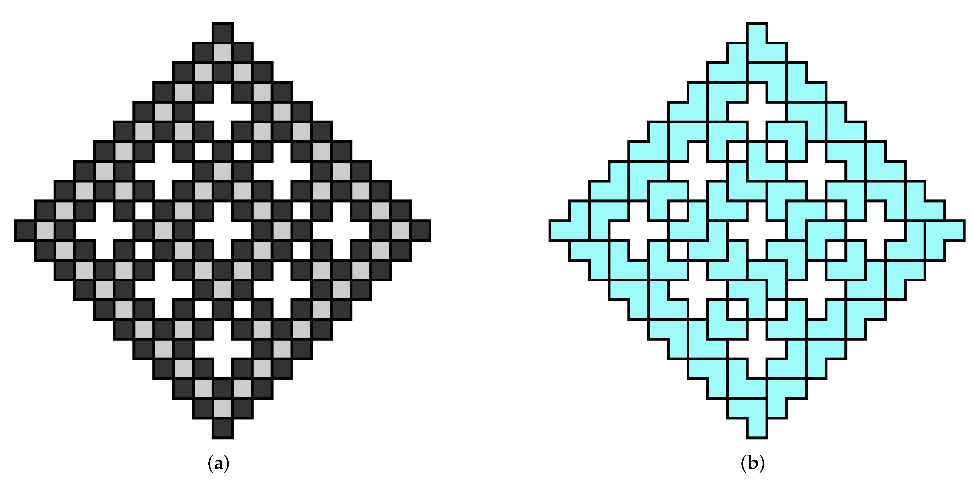
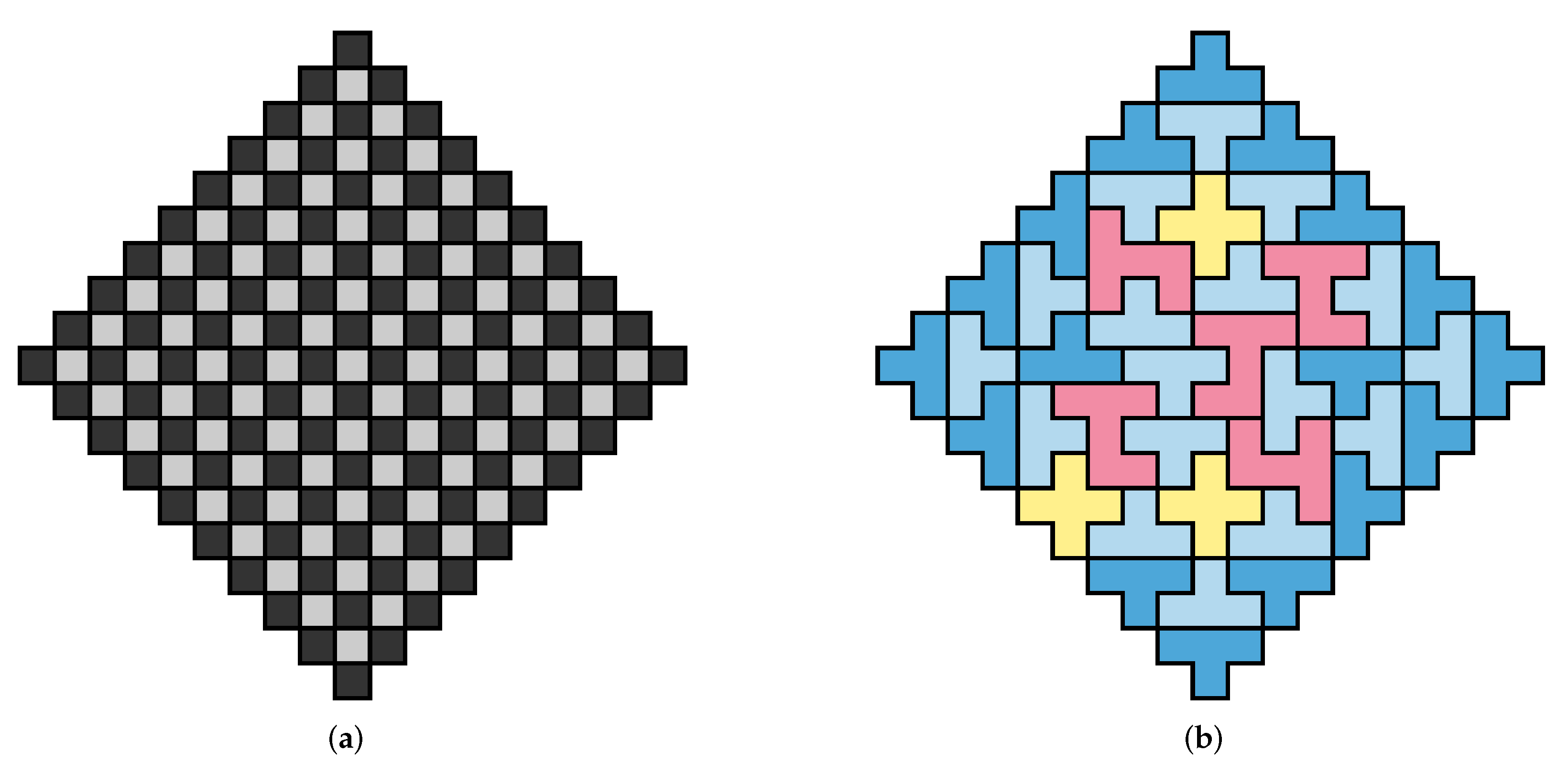
Find all ways of tiling the diamond shaped region with ‘holes’![Algorithms 15 00164 i011]() all orientations permitted. The area of R is 168, so we need 56 copies of the L-shaped trimino. The associated ILP file, constructed with the program LPMAKE_POLYOMINOES_FIGURE5, has n = 336 unknowns, m = 168 constraints, and f = 168 free variables. CPLEX found 16 solutions in 0.05 s.
all orientations permitted. The area of R is 168, so we need 56 copies of the L-shaped trimino. The associated ILP file, constructed with the program LPMAKE_POLYOMINOES_FIGURE5, has n = 336 unknowns, m = 168 constraints, and f = 168 free variables. CPLEX found 16 solutions in 0.05 s.
 all orientations permitted. The area of R is 168, so we need 56 copies of the L-shaped trimino. The associated ILP file, constructed with the program LPMAKE_POLYOMINOES_FIGURE5, has n = 336 unknowns, m = 168 constraints, and f = 168 free variables. CPLEX found 16 solutions in 0.05 s.
Using colouring techniques we wish to tile the checkerboard coloured regionshown in Figure 16a using 56 pariominoes from the set![Algorithms 15 00164 i012]() with parities , all orientations permitted. The parity of is , thus the only way to satisfy the parity equation (see Theorem 1) is to choose and . That is, the only way to tile is to use the pariominoes and we have a single pariomino tiling subproblem. We constructed the ILP file using the program LPMAKE_PARIOMINOES_FIGURE5. CPLEX found 16 solutions with in 0.02 s, thus the potential speedup when using the colouring technique is about 2.5×. However, as the runtimes are very small, this is not a particularly meaningful measure. The optimal solution of the pariomino tiling subproblem is shown in Figure 16b.
with parities , all orientations permitted. The parity of is , thus the only way to satisfy the parity equation (see Theorem 1) is to choose and . That is, the only way to tile is to use the pariominoes and we have a single pariomino tiling subproblem. We constructed the ILP file using the program LPMAKE_PARIOMINOES_FIGURE5. CPLEX found 16 solutions with in 0.02 s, thus the potential speedup when using the colouring technique is about 2.5×. However, as the runtimes are very small, this is not a particularly meaningful measure. The optimal solution of the pariomino tiling subproblem is shown in Figure 16b.
 with parities , all orientations permitted. The parity of is , thus the only way to satisfy the parity equation (see Theorem 1) is to choose and . That is, the only way to tile is to use the pariominoes and we have a single pariomino tiling subproblem. We constructed the ILP file using the program LPMAKE_PARIOMINOES_FIGURE5. CPLEX found 16 solutions with in 0.02 s, thus the potential speedup when using the colouring technique is about 2.5×. However, as the runtimes are very small, this is not a particularly meaningful measure. The optimal solution of the pariomino tiling subproblem is shown in Figure 16b.
Observe that for the polyomino tiling problem, we have n = 336 and for the pariomino tiling subproblem we have n = 224, which represent the number of ways fits in R and fits in , respectively. Thus, the number of ways fits in is , even though the single tiling solution uses only pariominoes of type .
Figure 16.
Target region and a tiling solution for Example 4: (a) the target region , a checkerboard coloured irregularly shaped region with ‘holes’; (b) successful tiling of the target region using 56 copies of an L-shaped trimino. The variants are coloured light-blue corresponding to an optimal solution of the single pariomino tiling subproblem.

Example 5.
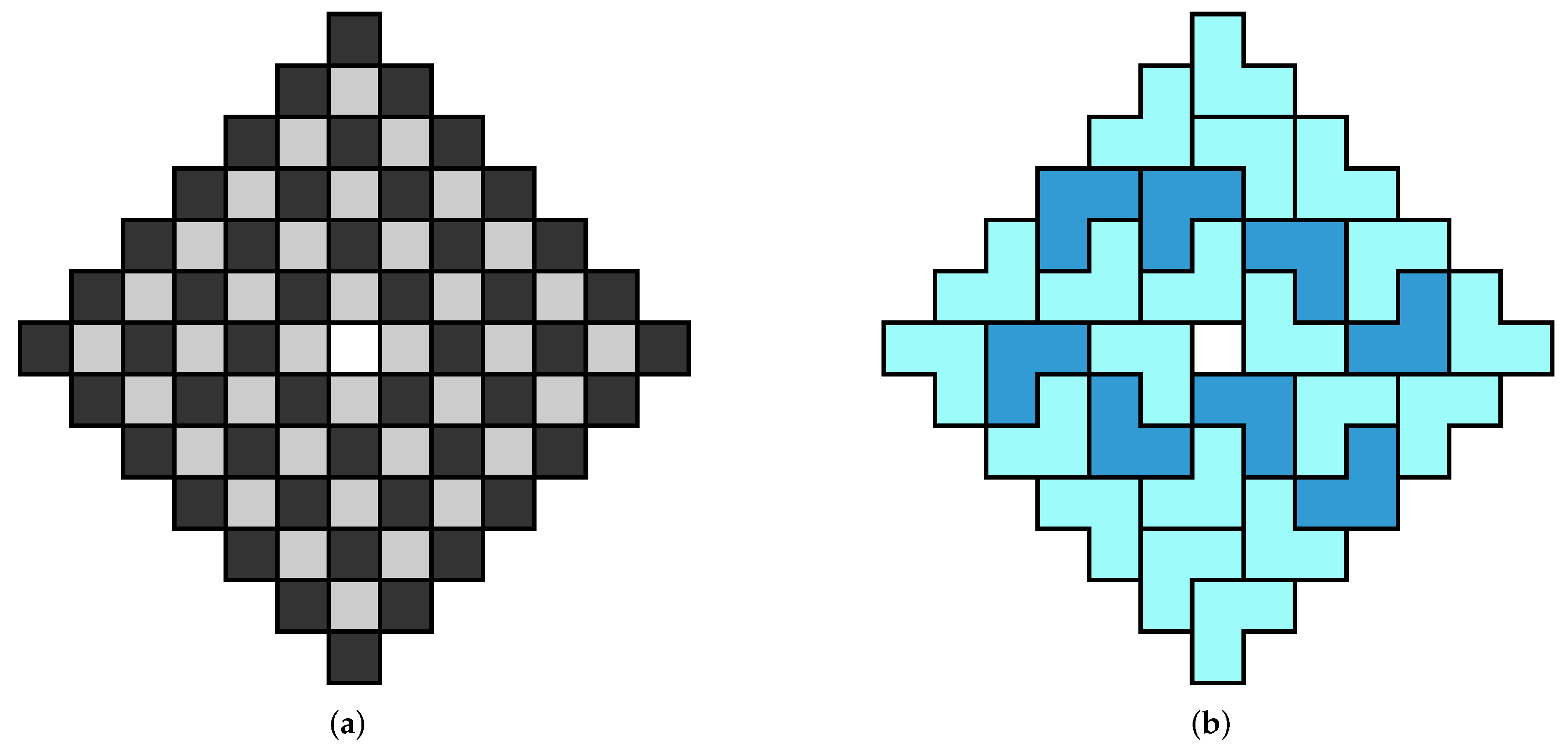
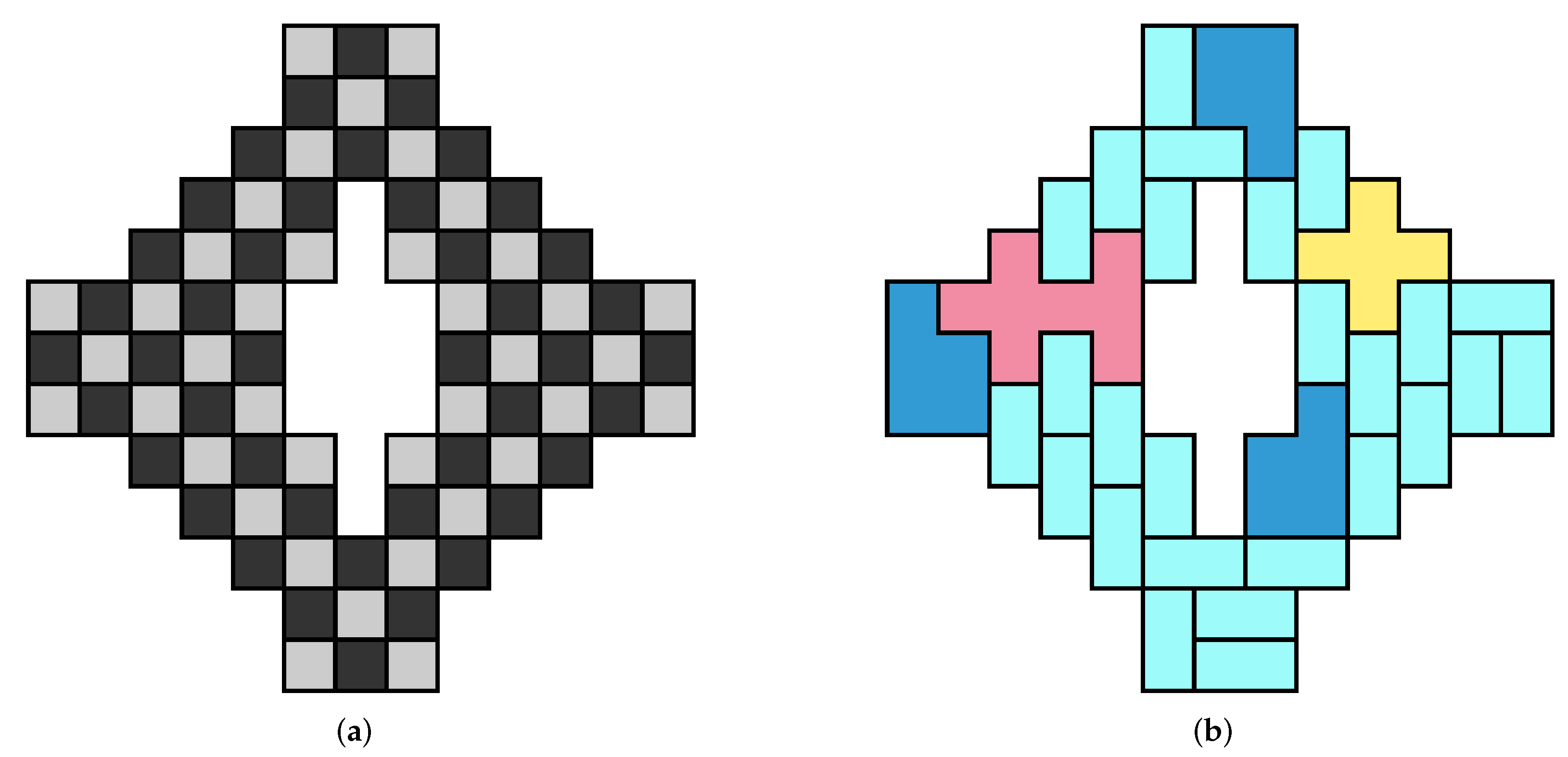
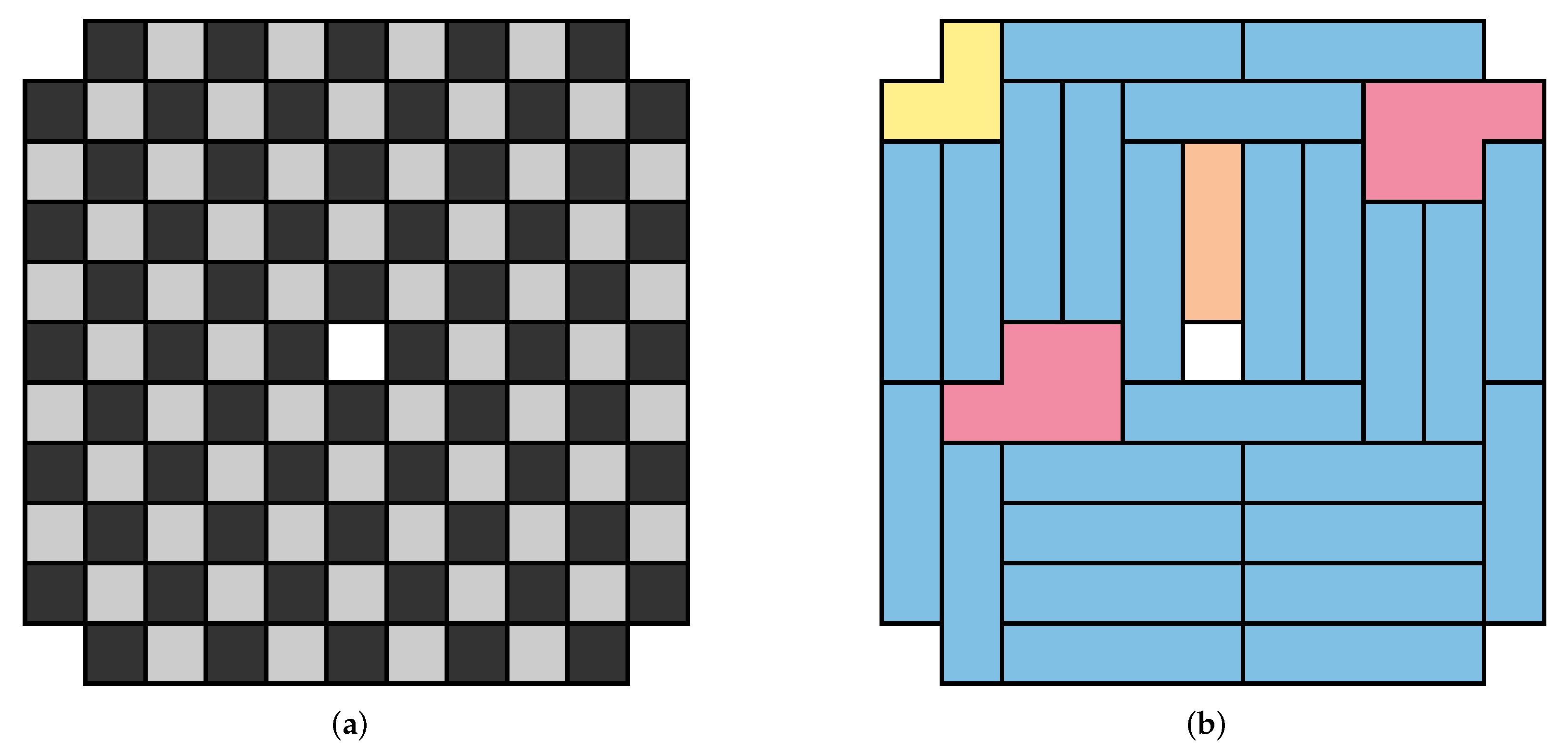
Find all ways of tiling the diamond shaped region with a single ‘hole’ in the middle![Algorithms 15 00164 i013]() all orientations permitted. The area of R is 84, so we need 28 copies of the L-shaped trimino. The associated ILP file, constructed with the programLPMAKE_POLYOMINOES_FIGURE6, has n = 252 unknowns, m = 84 constraints, and f = 168 free variables.CPLEX found 731,092 solutions in 165.78 s.
all orientations permitted. The area of R is 84, so we need 28 copies of the L-shaped trimino. The associated ILP file, constructed with the programLPMAKE_POLYOMINOES_FIGURE6, has n = 252 unknowns, m = 84 constraints, and f = 168 free variables.CPLEX found 731,092 solutions in 165.78 s.
 all orientations permitted. The area of R is 84, so we need 28 copies of the L-shaped trimino. The associated ILP file, constructed with the programLPMAKE_POLYOMINOES_FIGURE6, has n = 252 unknowns, m = 84 constraints, and f = 168 free variables.CPLEX found 731,092 solutions in 165.78 s.
Using colouring techniques we wish to tile the checkerboard coloured region shown in Figure 17a using 28 pariominoes from the set![Algorithms 15 00164 i014]() with parities , all orientations permitted. The parity of is , thus, the only way to satisfy the parity equation (see Theorem 1) is to choose and , i.e., we have a single pariomino tiling subproblem using 20 copies of and 8 copies of . The ILP file was constructed using the program LPMAKE_PARIOMINOES_FIGURE6. Solving this subproblem in CPLEX yielded 731,092 solutions with in 156.20 s, thus the potential speedup when using the colouring technique is about 1.1×. The optimal solution of the pariomino tiling subproblem is shown in Figure 17b.
with parities , all orientations permitted. The parity of is , thus, the only way to satisfy the parity equation (see Theorem 1) is to choose and , i.e., we have a single pariomino tiling subproblem using 20 copies of and 8 copies of . The ILP file was constructed using the program LPMAKE_PARIOMINOES_FIGURE6. Solving this subproblem in CPLEX yielded 731,092 solutions with in 156.20 s, thus the potential speedup when using the colouring technique is about 1.1×. The optimal solution of the pariomino tiling subproblem is shown in Figure 17b.
 with parities , all orientations permitted. The parity of is , thus, the only way to satisfy the parity equation (see Theorem 1) is to choose and , i.e., we have a single pariomino tiling subproblem using 20 copies of and 8 copies of . The ILP file was constructed using the program LPMAKE_PARIOMINOES_FIGURE6. Solving this subproblem in CPLEX yielded 731,092 solutions with in 156.20 s, thus the potential speedup when using the colouring technique is about 1.1×. The optimal solution of the pariomino tiling subproblem is shown in Figure 17b.
Figure 17.
Target region and a tiling solution for Example 5: (a) The target region , a checkerboard coloured diamond shaped region with a single ‘hole’ in the middle; (b) Successful tiling of the target region using 28 copies of an L-shaped trimino. The 20 pariominoes are coloured light-blue and the 8 pariominoes are coloured dark-blue, corresponding to an optimal solution of the single pariomino tiling subproblem.

6.2.4. Case 4
We give an example of the monohedral polyomino type, where the application of colouring techniques does not split the full (uncoloured) polyomino tiling problem into multiple pariomino tiling subproblems, and there is no reduction in complexity.
Example 6.
Find all ways of tiling the 16 × 18 rectangle with![Algorithms 15 00164 i015]() all orientations permitted. The area of R is 288, so we need 48 copies of the hexomino. The associated ILP file, constructed with the program LPMAKE_POLYOMINOES_FIGURE7, has n = 892 unknowns, m = 288 constraints, and f = 609 free variables. CPLEX found 217,266 solutions in 45.55 s.
all orientations permitted. The area of R is 288, so we need 48 copies of the hexomino. The associated ILP file, constructed with the program LPMAKE_POLYOMINOES_FIGURE7, has n = 892 unknowns, m = 288 constraints, and f = 609 free variables. CPLEX found 217,266 solutions in 45.55 s.
 all orientations permitted. The area of R is 288, so we need 48 copies of the hexomino. The associated ILP file, constructed with the program LPMAKE_POLYOMINOES_FIGURE7, has n = 892 unknowns, m = 288 constraints, and f = 609 free variables. CPLEX found 217,266 solutions in 45.55 s.
Using colouring techniques, we wish to tile the checkerboard coloured regionshown in Figure 18a using 48 pariominoes from the set![Algorithms 15 00164 i016]() all orientations permitted. We note here thatand so we only tile with copies of a single pariomino.
all orientations permitted. We note here thatand so we only tile with copies of a single pariomino.
 all orientations permitted. We note here thatand so we only tile with copies of a single pariomino.
As the hexomino and R have zero parity, the parity equation (see Theorem 1) is trivially satisfied and we obtain a single pariomino tiling subproblem. We constructed the ILP file in this case, using the program LPMAKE_PARIOMINOES_FIGURE7. Solving this subproblem in CPLEX with yielded 217,266 solutions in 50.75 s, i.e., an increase in the runtime of approximately 11.42% compared to the full (uncoloured) tiling problem. Thus we do not observe a potential speedup. An optimal solution of the pariomino tiling subproblem is illustrated in Figure 18b.
The pariomino tiling subproblem is essentially equivalent to the full polyomino tiling problem. Both formulations have the same binary matrices and no constraints of the form (4). Thus, the difference in the time taken for CPLEX to solve the polyomino tiling problem and the pariomino tiling subproblem is simply because of differences in the ordering of the unknowns in the binary linear systems. This results from the different order in which the binary matrices are constructed by our MATLAB programs for the polyomino and pariomino tiling cases. This situation also applies to any monohedral tiling problem where (so , for example, any pure domino tiling problem.
Figure 18.
Target region and a tiling solution for Example 6: (a) the target region , a rectangle; (b) successful tiling of the target region using 48 pariominoes (), coloured light-blue, corresponding to an optimal solution of the single pariomino tiling subproblem.
Figure 18.
Target region and a tiling solution for Example 6: (a) the target region , a rectangle; (b) successful tiling of the target region using 48 pariominoes (), coloured light-blue, corresponding to an optimal solution of the single pariomino tiling subproblem.

6.2.5. Case 5
We give four examples of the multihedral type, where the application of colouring techniques splits the full (uncoloured) polyomino tiling problem into multiple pariomino tiling subproblems, with a reduction in complexity.
Example 7.
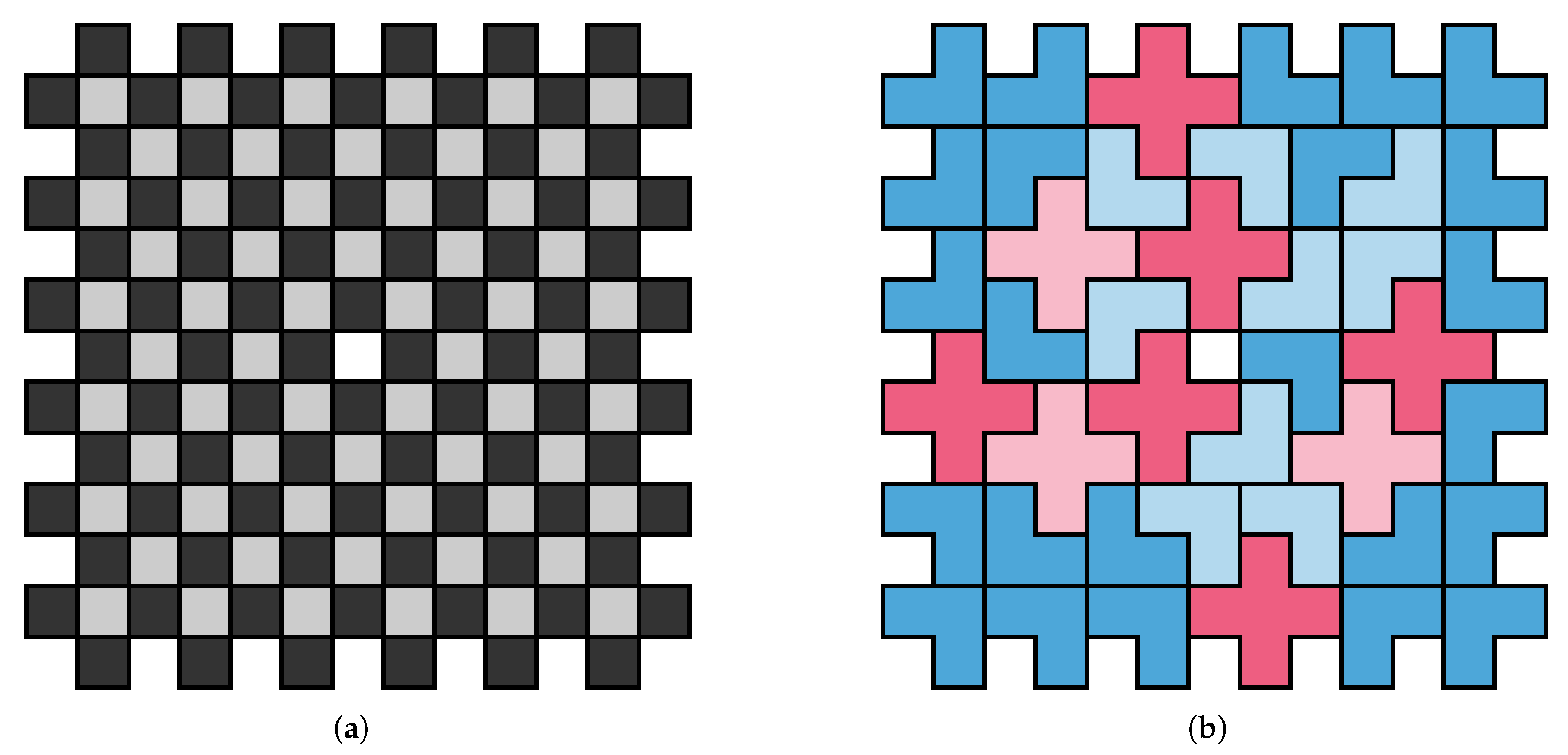
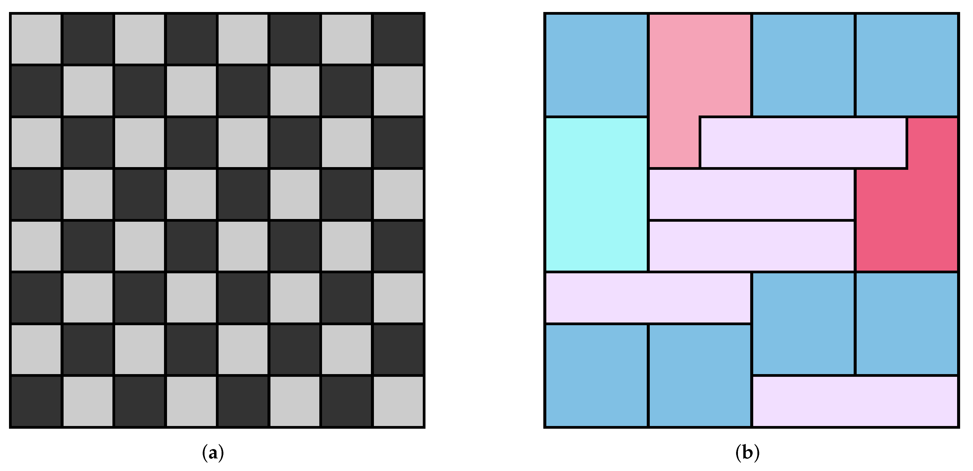
Find all ways of tiling the jagged-square shaped region with a single ‘hole’ in the middle![Algorithms 15 00164 i017]() all orientations permitted. The area of R is 144, which we aim to tile using= 33 copies of an L-shaped trimino and= 9 copies of the cross-shaped pentomino. The associated ILP file, constructed with the program
LPMAKE_POLYOMINOES_FIGURE8, has n = 528 unknowns, m = 146 constraints, and f = 383 free variables.
CPLEX
found 731,092 solutions in 165.78 s.
all orientations permitted. The area of R is 144, which we aim to tile using= 33 copies of an L-shaped trimino and= 9 copies of the cross-shaped pentomino. The associated ILP file, constructed with the program
LPMAKE_POLYOMINOES_FIGURE8, has n = 528 unknowns, m = 146 constraints, and f = 383 free variables.
CPLEX
found 731,092 solutions in 165.78 s.
 all orientations permitted. The area of R is 144, which we aim to tile using= 33 copies of an L-shaped trimino and= 9 copies of the cross-shaped pentomino. The associated ILP file, constructed with the program
LPMAKE_POLYOMINOES_FIGURE8, has n = 528 unknowns, m = 146 constraints, and f = 383 free variables.
CPLEX
found 731,092 solutions in 165.78 s.
all orientations permitted. The area of R is 144, which we aim to tile using= 33 copies of an L-shaped trimino and= 9 copies of the cross-shaped pentomino. The associated ILP file, constructed with the program
LPMAKE_POLYOMINOES_FIGURE8, has n = 528 unknowns, m = 146 constraints, and f = 383 free variables.
CPLEX
found 731,092 solutions in 165.78 s.Using colouring techniques, we wish to tile the checkerboard coloured regionshown in Figure 19a using 33 pariominoes from the set![Algorithms 15 00164 i018]() with parities, and 9 pariominoes from the set
with parities, and 9 pariominoes from the set![Algorithms 15 00164 i019]() with parities, all orientations permitted. The parity equation (see Theorem 1) is given by
with parities, all orientations permitted. The parity equation (see Theorem 1) is given by
 with parities, and 9 pariominoes from the set
 with parities, all orientations permitted. The parity equation (see Theorem 1) is given by
After noting that we obtain the linear Diophantine equation
The MATLAB
program DIOPHANTINE_ND_NONNEGATIVE_BOUNDED was used to solve this equation yielding seven pariomino tiling subproblems, solved in CPLEX
to give the data in Table 3 for the number of pariomino tiling solutions (# solns.) and
CPLEX
runtimes (sec).
Figure 19.
Target region and a tiling solution for Example 7: (a) The target region , a checkerboard coloured jagged-square shaped region with a single ‘hole’ in the middle. (b) Successful tiling of the target region using 33 copies of an L-shaped trimino and 9 copies of the cross-shaped pentomino. The optimal solution corresponds to the fourth pariomino tiling subproblem in Table 3 where we use 24 copies of , 9 copies of , 6 copies of , and 3 copies of . The pariominoes and are coloured dark blue, light blue, dark red, and light red, respectively.

Table 3.
Number of tiling solutions (# solns.) and runtimes in seconds for CPLEX to solve the seven pariomino tiling subproblems in Example 7.
Table 3.
Number of tiling solutions (# solns.) and runtimes in seconds for CPLEX to solve the seven pariomino tiling subproblems in Example 7.
| n | m | f | # Solns. | Runtime (s) | ||
| 15 | 9 | 492 | 147 | 347 | - | 0.00 |
| 18 | 8 | 528 | 148 | 382 | - | 0.04 |
| 21 | 7 | 528 | 148 | 382 | - | 0.04 |
| 24 | 6 | 528 | 148 | 382 | 62,960 | 15.21 |
| 27 | 5 | 528 | 148 | 382 | 339,224 | 106.42 |
| 30 | 4 | 528 | 148 | 382 | 16,256 | 2.84 |
| 33 | 3 | 336 | 147 | 191 | - | 0.10 |
The fifth subproblem took the longest to solve (106.42 s), thus the potential speedup when using the colouring technique is about 1.6×. We found an optimal solution using
CPLEX
for the fourth subproblem, i.e., using 24 copies of , 9 copies of , 6 copies of , and 3 copies of (see Figure 19b). We constructed the ILP file in this case, using the program
LPMAKE_PARIOMINOES_FIGURE8 (similar programs were used to construct the ILP files for the other cases).
Example 8.
Find all ways of tiling the diamond-shaped region![Algorithms 15 00164 i020]() all orientations permitted. The area of R is 181, which we aim to tile using= 34 copies of the T-shaped trimino,= 5 copies of Y-shaped hexomino, and= 3 copies of the cross-shaped pentomino. The ILP file, constructed with the program
LPMAKE_POLYOMINOES_FIGURE9, has n = 1685 unknowns, m = 184 constraints, and f = 1502 free variables.
CPLEX
found 337,680 solutions in 225.06 s.
all orientations permitted. The area of R is 181, which we aim to tile using= 34 copies of the T-shaped trimino,= 5 copies of Y-shaped hexomino, and= 3 copies of the cross-shaped pentomino. The ILP file, constructed with the program
LPMAKE_POLYOMINOES_FIGURE9, has n = 1685 unknowns, m = 184 constraints, and f = 1502 free variables.
CPLEX
found 337,680 solutions in 225.06 s.
 all orientations permitted. The area of R is 181, which we aim to tile using= 34 copies of the T-shaped trimino,= 5 copies of Y-shaped hexomino, and= 3 copies of the cross-shaped pentomino. The ILP file, constructed with the program
LPMAKE_POLYOMINOES_FIGURE9, has n = 1685 unknowns, m = 184 constraints, and f = 1502 free variables.
CPLEX
found 337,680 solutions in 225.06 s.
all orientations permitted. The area of R is 181, which we aim to tile using= 34 copies of the T-shaped trimino,= 5 copies of Y-shaped hexomino, and= 3 copies of the cross-shaped pentomino. The ILP file, constructed with the program
LPMAKE_POLYOMINOES_FIGURE9, has n = 1685 unknowns, m = 184 constraints, and f = 1502 free variables.
CPLEX
found 337,680 solutions in 225.06 s.Using colouring techniques we wish to tile the checkerboard coloured regionshown in Figure 20a using 34 pariominoes from the set![Algorithms 15 00164 i021]() with parities, and 5 pariominoes from the set
with parities, and 5 pariominoes from the set![Algorithms 15 00164 i022]() with parities, and 3 pariominoes from the set
with parities, and 3 pariominoes from the set![Algorithms 15 00164 i023]() with parities, all orientations permitted. The parity equation (see Theorem 1) is given by
with parities, all orientations permitted. The parity equation (see Theorem 1) is given by
 with parities, and 5 pariominoes from the set
 with parities, and 3 pariominoes from the set
 with parities, all orientations permitted. The parity equation (see Theorem 1) is given by
After noting that we obtain the linear Diophantine equation
The
MATLAB
program
DIOPHANTINE_ND_NONNEGATIVE_BOUNDED
was used to solve this equation yielding 12 pariomino tiling subproblems, solved in
CPLEX
to give the data in Table 4 for the number of pariomino tiling solutions and
CPLEX
runtimes.
The sixth subproblem took the longest to solve (72.09 s), and thus the potential speedup when using the colouring technique is about 3.1×. We found an optimal solution using
CPLEX
for the first subproblem, i.e., using 17 copies of , 17 copies of , 5 copies of , and 3 copies of (see Figure 20b). We constructed the ILP file in this case using the program
LPMAKE_PARIOMINOES_FIGURE9
(similar programs were used to construct the ILP files for the other cases).
Table 4.
Number of tiling solutions (# solns.) and runtimes in seconds for CPLEX to solve the 12 pariomino tiling subproblems in Example 8.
Table 4.
Number of tiling solutions (# solns.) and runtimes in seconds for CPLEX to solve the 12 pariomino tiling subproblems in Example 8.
| n | m | f | # Solns. | Runtime (s) | |||
| 17 | 5 | 3 | 1173 | 185 | 990 | 344 | 0.53 |
| 18 | 4 | 3 | 1621 | 186 | 1437 | 7528 | 8.32 |
| 19 | 3 | 3 | 1621 | 186 | 1437 | 53,144 | 43.81 |
| 20 | 2 | 3 | 1621 | 186 | 1437 | 125,104 | 72.01 |
| 20 | 5 | 1 | 1237 | 186 | 1053 | - | 0.39 |
| 21 | 1 | 3 | 1621 | 186 | 1437 | 117,192 | 72.09 |
| 21 | 4 | 1 | 1685 | 187 | 1500 | - | 1.64 |
| 22 | 0 | 3 | 1109 | 185 | 926 | 34,272 | 15.00 |
| 22 | 3 | 1 | 1685 | 187 | 1500 | 32 | 3.57 |
| 23 | 2 | 1 | 1685 | 187 | 1500 | 64 | 3.09 |
| 24 | 1 | 1 | 1685 | 187 | 1500 | - | 1.59 |
| 25 | 0 | 1 | 1173 | 186 | 989 | - | 0.68 |
Figure 20.
Target region and a tiling solution for Example 8: (a) the target region , a checkerboard coloured diamond-shaped region; (b) successful tiling of the target region using 34 copies of a T-shaped trimino, 5 copies of the Y-shaped hexomino, and 3 copies of the cross-shaped pentomino. The optimal solution corresponds to the first pariomino tiling subproblem in Table 4 using 17 copies of , 17 copies of , 5 copies of , and 3 copies of . The pariominoes , , , and are coloured dark blue, light blue, red, and yellow, respectively.

Example 9.
Find all ways of tiling the region![Algorithms 15 00164 i024]() all orientations permitted. The area of R is 80, which we aim to tile with= 26 copies of the domino,= 3 copies of the P-shaped pentomino,= 1 copies of the cross-shaped pentomino, and= 1 copies of the octomino. The associated ILP file, constructed with the program
LPMAKE_POLYOMINOES_FIGURE10, has n = 444 unknowns, m = 84 constraints, and f = 361 free variables.
CPLEX
found 105,344 solutions in 16.83 s.
all orientations permitted. The area of R is 80, which we aim to tile with= 26 copies of the domino,= 3 copies of the P-shaped pentomino,= 1 copies of the cross-shaped pentomino, and= 1 copies of the octomino. The associated ILP file, constructed with the program
LPMAKE_POLYOMINOES_FIGURE10, has n = 444 unknowns, m = 84 constraints, and f = 361 free variables.
CPLEX
found 105,344 solutions in 16.83 s.
 all orientations permitted. The area of R is 80, which we aim to tile with= 26 copies of the domino,= 3 copies of the P-shaped pentomino,= 1 copies of the cross-shaped pentomino, and= 1 copies of the octomino. The associated ILP file, constructed with the program
LPMAKE_POLYOMINOES_FIGURE10, has n = 444 unknowns, m = 84 constraints, and f = 361 free variables.
CPLEX
found 105,344 solutions in 16.83 s.
all orientations permitted. The area of R is 80, which we aim to tile with= 26 copies of the domino,= 3 copies of the P-shaped pentomino,= 1 copies of the cross-shaped pentomino, and= 1 copies of the octomino. The associated ILP file, constructed with the program
LPMAKE_POLYOMINOES_FIGURE10, has n = 444 unknowns, m = 84 constraints, and f = 361 free variables.
CPLEX
found 105,344 solutions in 16.83 s.Using colouring techniques, we wish to tile the checkerboard coloured regionshown in Figure 21a using 26 pariominoes from the set![Algorithms 15 00164 i025]() with parity, (), and three pariominoes from the set
with parity, (), and three pariominoes from the set![Algorithms 15 00164 i026]() with parities, and one pariomino from the set
with parities, and one pariomino from the set![Algorithms 15 00164 i027]() with parities, and one pariomino from the set
with parities, and one pariomino from the set![Algorithms 15 00164 i028]() with parities, all orientations permitted.
with parities, all orientations permitted.
 with parity, (), and three pariominoes from the set
 with parities, and one pariomino from the set
 with parities, and one pariomino from the set
 with parities, all orientations permitted.
Figure 21.
Target region and a tiling solution for Example 9: (a) The checkerboard coloured target region ; (b) Successful tiling of the target region using 26 copies of a domino, 3 copies of the P-shaped pentomino, one copy of the cross-shaped pentomino, and one copy of an octomino. The optimal solution corresponds to the first pariomino tiling subproblem in Table 5 using 26 copies of , three copies of , one copy of , and one copy of . The pariominoes , , , and are coloured light blue, blue, yellow and red, respectively.

The parity equation (see Theorem 1) is given by
After noting that , we obtain the linear Diophantine equation
The
MATLAB
program
DIOPHANTINE_ND_NONNEGATIVE_BOUNDED
was used to solve this equation, yielding 2 pariomino tiling subproblems, solved in
CPLEX
to give the data in Table 5 for the number of pariomino tiling solutions and
CPLEX
runtimes.
The first (and only feasible) subproblem took 14.28 s to solve, thus the potential speedup when using the colouring technique is about 1.2×. We constructed the ILP file, in this case, using the program
LPMAKE_PARIOMINOES_FIGURE10
. We found an optimal solution using
CPLEX
for the first subproblem, i.e., using 26 copies of , three copies of , one copy of , and one copy of (see Figure 21b).
Example 10.
Find all ways of tiling the 8 × 16 rectangle using the following octominoes![Algorithms 15 00164 i029]() all orientations permitted, with the following numbers of copies:
The sum of the areas of the tilesequals the area of the target region as required. The associated ILP file, constructed with the program
LPMAKE_POLYOMINOES_FIGURE11, has n = 3126 unknowns, m = 138 constraints, and f = 2989 free variables.
CPLEX
found 96 solutions in 163.95 s.
all orientations permitted, with the following numbers of copies:
The sum of the areas of the tilesequals the area of the target region as required. The associated ILP file, constructed with the program
LPMAKE_POLYOMINOES_FIGURE11, has n = 3126 unknowns, m = 138 constraints, and f = 2989 free variables.
CPLEX
found 96 solutions in 163.95 s.
 all orientations permitted, with the following numbers of copies:
Using colouring techniques, we wish to tile the checkerboard coloured regionshown in Figure 22a, usingpariominoes from the setsfor i = 1, 2, …, 7, andpariominoes from the setsfor j = 8, 9, 10, with
![Algorithms 15 00164 i030]() all orientations permitted, wherefor i = 1, 2, …, 7 andfor j = 8, 9, 10. The parities of the pariominoes are given by
all orientations permitted, wherefor i = 1, 2, …, 7 andfor j = 8, 9, 10. The parities of the pariominoes are given by
 all orientations permitted, wherefor i = 1, 2, …, 7 andfor j = 8, 9, 10. The parities of the pariominoes are given by
Figure 22.
Target region and a tiling solution for Example 10: (a) The target region , a checkerboard coloured rectangle; (b) Successful tiling of the target region using 16 octominoes. The optimal solution corresponds to the first pariomino tiling subproblem in Table 6 with . The pariomino is coloured dark green to distinguish it from , which is coloured light green.

The parity equation (see Theorem 1) is given by
After noting that we obtain the linear Diophantine equation
The
MATLAB
program
DIOPHANTINE_ND_NONNEGATIVE_BOUNDED
was used to solve this equation yielding four pariomino tiling subproblems, solved in
CPLEX
to give the data in Table 6 for the number of pariomino tiling solutions and
CPLEX
runtimes.
The fourth subproblem took the longest to solve (54.14 s), thus the potential speedup when using the colouring technique is about 3.0×. We found an optimal solution using
CPLEX
for the first subproblem, i.e., using copies of the pariominoes for i = 1, 2, …, 7, two copies of , and one copy each of , and (see Figure 22b). We constructed the ILP file in this case using the program
LPMAKE_PARIOMINOES_FIGURE11
(similar programs were used to construct the ILP files for the other cases).
6.2.6. Case 6
We could not find an example of the multihedral type, where the application of colouring techniques splits the full (uncoloured) polyomino tiling problem into multiple pariomino tiling subproblems and there is no reduction in complexity.
6.2.7. Case 7
We give an example of the multihedral polyomino type, where the application of colouring techniques does not split the full (uncoloured) polyomino tiling problem into multiple pariomino tiling subproblems and reduces the complexity.
Example 11.
Find all ways of tiling the notched square-shaped region with a single ‘hole’![Algorithms 15 00164 i031]() all orientations permitted. The area of R is 116, which we aim to tile using= 25 copies of the straight tetromino,= 1 copy of the straight trimino,= 1 copy of the L-shaped trimino, and= 2 copies of the P-shaped pentomino. The associated ILP file, constructed with the program LPMAKE_POLYOMINOES_FIGURE12, has n = 1376 unknowns, m = 120 constraints, and f = 1257 free variables.
CPLEX
found 429,800 solutions in 768.74 s.
all orientations permitted. The area of R is 116, which we aim to tile using= 25 copies of the straight tetromino,= 1 copy of the straight trimino,= 1 copy of the L-shaped trimino, and= 2 copies of the P-shaped pentomino. The associated ILP file, constructed with the program LPMAKE_POLYOMINOES_FIGURE12, has n = 1376 unknowns, m = 120 constraints, and f = 1257 free variables.
CPLEX
found 429,800 solutions in 768.74 s.
 all orientations permitted. The area of R is 116, which we aim to tile using= 25 copies of the straight tetromino,= 1 copy of the straight trimino,= 1 copy of the L-shaped trimino, and= 2 copies of the P-shaped pentomino. The associated ILP file, constructed with the program LPMAKE_POLYOMINOES_FIGURE12, has n = 1376 unknowns, m = 120 constraints, and f = 1257 free variables.
CPLEX
found 429,800 solutions in 768.74 s.
all orientations permitted. The area of R is 116, which we aim to tile using= 25 copies of the straight tetromino,= 1 copy of the straight trimino,= 1 copy of the L-shaped trimino, and= 2 copies of the P-shaped pentomino. The associated ILP file, constructed with the program LPMAKE_POLYOMINOES_FIGURE12, has n = 1376 unknowns, m = 120 constraints, and f = 1257 free variables.
CPLEX
found 429,800 solutions in 768.74 s.Using colouring techniques, we wish to tile the checkerboard coloured regionshown in Figure 23a using 25 pariominoes from the set![Algorithms 15 00164 i032]() with parity, (), and one pariomino from the set
with parity, (), and one pariomino from the set![Algorithms 15 00164 i033]() with parities, and one pariomino from the set
with parities, and one pariomino from the set![Algorithms 15 00164 i034]() with parities, and two pariomino from the set
with parities, and two pariomino from the set![Algorithms 15 00164 i035]() with parities, all orientations permitted. As the parity ofis, the only way to satisfy the parity equation (see Theorem 1) is to choose 25 copies of(=), one copy of, one copy of, and two copies of. We constructed the ILP file in this case using the program
LPMAKE_PARIOMINOES_FIGURE12. Solving this single subproblem in
CPLEX
withyielded 429,800 solutions in 156.46 s, thus the potential speedup when using the colouring technique is about 4.9×. An optimal solution of this pariomino tiling subproblem is illustrated in Figure 23b.
with parities, all orientations permitted. As the parity ofis, the only way to satisfy the parity equation (see Theorem 1) is to choose 25 copies of(=), one copy of, one copy of, and two copies of. We constructed the ILP file in this case using the program
LPMAKE_PARIOMINOES_FIGURE12. Solving this single subproblem in
CPLEX
withyielded 429,800 solutions in 156.46 s, thus the potential speedup when using the colouring technique is about 4.9×. An optimal solution of this pariomino tiling subproblem is illustrated in Figure 23b.
 with parity, (), and one pariomino from the set
 with parities, and one pariomino from the set
 with parities, and two pariomino from the set
 with parities, all orientations permitted. As the parity ofis, the only way to satisfy the parity equation (see Theorem 1) is to choose 25 copies of(=), one copy of, one copy of, and two copies of. We constructed the ILP file in this case using the program
LPMAKE_PARIOMINOES_FIGURE12. Solving this single subproblem in
CPLEX
withyielded 429,800 solutions in 156.46 s, thus the potential speedup when using the colouring technique is about 4.9×. An optimal solution of this pariomino tiling subproblem is illustrated in Figure 23b.
with parities, all orientations permitted. As the parity ofis, the only way to satisfy the parity equation (see Theorem 1) is to choose 25 copies of(=), one copy of, one copy of, and two copies of. We constructed the ILP file in this case using the program
LPMAKE_PARIOMINOES_FIGURE12. Solving this single subproblem in
CPLEX
withyielded 429,800 solutions in 156.46 s, thus the potential speedup when using the colouring technique is about 4.9×. An optimal solution of this pariomino tiling subproblem is illustrated in Figure 23b.
Figure 23.
Target region and a tiling solution for Example 11: (a) the target region , a checkerboard coloured ‘4-notched square shape’ with a single ‘hole’ in the middle; (b) successful tiling of the target region using 25 copies of the straight tetromino, one copy of the straight trimino, one copy of the L-shaped trimino, and two copies of the P-shaped pentomino. The single optimal solution uses 25 copies of (=), one copy of , one copy of , and two copies of . The pariominoes , , , and are coloured blue, orange, yellow and red, respectively.

6.2.8. Case 8
We give an example of the multihedral polyomino type, where the application of colouring techniques does not split the full (uncoloured) polyomino tiling problem into multiple pariomino tiling subproblems, and there is no reduction in complexity.
Example 12.
Find all ways of tiling the 8 × 8 square with![Algorithms 15 00164 i036]() all orientations permitted. We aim to tile R using= 5 copies of the straight tetromino,= 7 copies of the 2 × 2 square,= 1 copies of the 2 × 3 rectangle, and= 2 copies of the P-shaped pentomino. The ILP file, constructed with the program
LPMAKE_POLYOMINOES_FIGURE13, has n = 549 unknowns, m = 68 constraints, and f = 482 free variables.
CPLEX
found 157,288 solutions in 78 s.
all orientations permitted. We aim to tile R using= 5 copies of the straight tetromino,= 7 copies of the 2 × 2 square,= 1 copies of the 2 × 3 rectangle, and= 2 copies of the P-shaped pentomino. The ILP file, constructed with the program
LPMAKE_POLYOMINOES_FIGURE13, has n = 549 unknowns, m = 68 constraints, and f = 482 free variables.
CPLEX
found 157,288 solutions in 78 s.
 all orientations permitted. We aim to tile R using= 5 copies of the straight tetromino,= 7 copies of the 2 × 2 square,= 1 copies of the 2 × 3 rectangle, and= 2 copies of the P-shaped pentomino. The ILP file, constructed with the program
LPMAKE_POLYOMINOES_FIGURE13, has n = 549 unknowns, m = 68 constraints, and f = 482 free variables.
CPLEX
found 157,288 solutions in 78 s.
all orientations permitted. We aim to tile R using= 5 copies of the straight tetromino,= 7 copies of the 2 × 2 square,= 1 copies of the 2 × 3 rectangle, and= 2 copies of the P-shaped pentomino. The ILP file, constructed with the program
LPMAKE_POLYOMINOES_FIGURE13, has n = 549 unknowns, m = 68 constraints, and f = 482 free variables.
CPLEX
found 157,288 solutions in 78 s.Using colouring techniques, we wish to tile the checkerboard coloured regionshown in Figure 24a using five pariominoes from the set![Algorithms 15 00164 i037]() with parity, (), and seven pariominoes from the set
with parity, (), and seven pariominoes from the set![Algorithms 15 00164 i038]() with parities, (), and one pariomino from the set
with parities, (), and one pariomino from the set![Algorithms 15 00164 i039]() with parities, (), and two pariominoes from the set
with parities, (), and two pariominoes from the set![Algorithms 15 00164 i040]() with parities, all orientations permitted. As the parity ofis zero, the only way to satisfy the parity equation (see Theorem 1) is to choose five copies of(=), seven copies of(=), one copy of(=), and one copy each ofand. We constructed the ILP file in this case using the program
LPMAKE_PARIOMINOES_FIGURE13. Solving this single subproblem in
CPLEX
withyielded 157,288 solutions in 85.3 s, which is an increase in the runtime of about 9.4% compared to the full (uncoloured) tiling problem. Thus, no potential speedup is observed. An optimal solution of this pariomino tiling subproblem is illustrated in Figure 24b.
with parities, all orientations permitted. As the parity ofis zero, the only way to satisfy the parity equation (see Theorem 1) is to choose five copies of(=), seven copies of(=), one copy of(=), and one copy each ofand. We constructed the ILP file in this case using the program
LPMAKE_PARIOMINOES_FIGURE13. Solving this single subproblem in
CPLEX
withyielded 157,288 solutions in 85.3 s, which is an increase in the runtime of about 9.4% compared to the full (uncoloured) tiling problem. Thus, no potential speedup is observed. An optimal solution of this pariomino tiling subproblem is illustrated in Figure 24b.
 with parity, (), and seven pariominoes from the set
 with parities, (), and one pariomino from the set
 with parities, (), and two pariominoes from the set
 with parities, all orientations permitted. As the parity ofis zero, the only way to satisfy the parity equation (see Theorem 1) is to choose five copies of(=), seven copies of(=), one copy of(=), and one copy each ofand. We constructed the ILP file in this case using the program
LPMAKE_PARIOMINOES_FIGURE13. Solving this single subproblem in
CPLEX
withyielded 157,288 solutions in 85.3 s, which is an increase in the runtime of about 9.4% compared to the full (uncoloured) tiling problem. Thus, no potential speedup is observed. An optimal solution of this pariomino tiling subproblem is illustrated in Figure 24b.
with parities, all orientations permitted. As the parity ofis zero, the only way to satisfy the parity equation (see Theorem 1) is to choose five copies of(=), seven copies of(=), one copy of(=), and one copy each ofand. We constructed the ILP file in this case using the program
LPMAKE_PARIOMINOES_FIGURE13. Solving this single subproblem in
CPLEX
withyielded 157,288 solutions in 85.3 s, which is an increase in the runtime of about 9.4% compared to the full (uncoloured) tiling problem. Thus, no potential speedup is observed. An optimal solution of this pariomino tiling subproblem is illustrated in Figure 24b.
Figure 24.
Target region and a tiling solution for Example 12: (a) the target region , a checkerboard coloured square; (b) successful tiling of the target region using five copies of the straight tetromino, seven copies of the square, one copy of the rectangle, and two copies of the P-shaped pentomino. The single optimal solution uses five copies of (=), seven copies of (=), one copy of (=), and one copy each of and . The pariominoes , , , , and are coloured violet, blue, light blue, red, and light red, respectively.

6.3. Tiling Examples Where We Seek a Single Solution
In this section, we are concerned with finding a single (optimal) solution to the ILP problems associated with tiling. Using checkerboard colouring techniques, we are interested in the pariomino tiling subproblem that yields a feasible solution in the least amount of time. If this is less than the time to find an optimal solution for the full (uncoloured) tiling problem, then we have reduced the complexity of this tiling problem.
We give a single example to illustrate this approach.
Example 13.
Find a single way of tiling the 60 × 64 rectangle with![Algorithms 15 00164 i041]() all orientations permitted. We aim to tile R using= 384 copies of the V-shaped pentomino, and= 384 copies of the L-shaped pentomino. The associated ILP file, constructed with the program
LPMAKE_POLYOMINOES_FIGURE14, has n = 43,144 unknowns, m = 3842 constraints, and f = 39,303 free variables.
CPLEX
found an optimal solution in approximately 24 h.
all orientations permitted. We aim to tile R using= 384 copies of the V-shaped pentomino, and= 384 copies of the L-shaped pentomino. The associated ILP file, constructed with the program
LPMAKE_POLYOMINOES_FIGURE14, has n = 43,144 unknowns, m = 3842 constraints, and f = 39,303 free variables.
CPLEX
found an optimal solution in approximately 24 h.
 all orientations permitted. We aim to tile R using= 384 copies of the V-shaped pentomino, and= 384 copies of the L-shaped pentomino. The associated ILP file, constructed with the program
LPMAKE_POLYOMINOES_FIGURE14, has n = 43,144 unknowns, m = 3842 constraints, and f = 39,303 free variables.
CPLEX
found an optimal solution in approximately 24 h.
all orientations permitted. We aim to tile R using= 384 copies of the V-shaped pentomino, and= 384 copies of the L-shaped pentomino. The associated ILP file, constructed with the program
LPMAKE_POLYOMINOES_FIGURE14, has n = 43,144 unknowns, m = 3842 constraints, and f = 39,303 free variables.
CPLEX
found an optimal solution in approximately 24 h.Using colouring techniques, we wish to tile the 60 × 64 checkerboard coloured regionusing 384 pariominoes from the set![Algorithms 15 00164 i042]() with parities, and 384 pariominoes from the set
with parities, and 384 pariominoes from the set![Algorithms 15 00164 i043]() with parities, all orientations permitted. In the interests of space, we do not illustrate; however, it is sufficient to note that the top left square is white. The parity equation (see Theorem 1) is given by
with parities, all orientations permitted. In the interests of space, we do not illustrate; however, it is sufficient to note that the top left square is white. The parity equation (see Theorem 1) is given by
 with parities, and 384 pariominoes from the set
 with parities, all orientations permitted. In the interests of space, we do not illustrate; however, it is sufficient to note that the top left square is white. The parity equation (see Theorem 1) is given by
After noting that , we obtain the linear Diophantine equation
with 385 solutions . Due to time constraints, we only solved a single subproblem corresponding to , i.e., using 384 copies each of and . We constructed the ILP file in this case using the program
LPMAKE_PARIOMINOES_FIGURE14. Using
CPLEX
yielded an optimal solution in 2.6 h, with . Thus the potential speedup when using the colouring technique is at least 9.2×. The optimal solution is illustrated in Figure 25.
7. Performance Analysis
We make some observations about the numerical results presented in Section 6; however, it is hard to make general conclusions because of the many situations that arise (see Figure 12). Some problems do not split into subproblems, or do not do so usefully. We give a summary of the potential speedup results in Table 7.
Most problems do split into multiple, smaller subproblems. This has advantages if we are seeking a single solution, or all solutions because we can work in parallel. When a problem splits into multiple pariomino tiling subproblems, the experiments show that the CPLEX runtimes for the subproblems roughly correlate with the number of solutions found (see Example 8). Thus a subproblem with the greatest runtime is more likely to be small compared to the runtime of the full problem if the total number of solutions is uniformly distributed among the subproblems. We also saw that the runtimes for infeasible subproblems were much less than the runtimes for the feasible ones.
How a problem splits into subproblems depends on whether we are working with a multihedral or monohedral tiling problem. There are two different situations that yield a splitting of a polyomino tiling problem into multiple pariomino tiling subproblems. In the monohedral case, when tiling with copies of a polyomino where and , we automatically obtain subproblems to consider (see Example 1). The second situation that yields a splitting is in the multihedral case, where the parity equation in Theorem 1 has multiple solutions. However, we can easily create multihedral problems that do not split by using mostly tiles where and hence . For example, Example 12 behaves essentially like a monohedral problem with two P-shaped pentominoes, as zero parity tiles play no part in the parity equation of Theorem 1. In the monohedral case when using tiles with non-zero parity, or where (so ), the parity equation is trivially solved, which implies there is no splitting of the polyomino tiling problem.
The numerical results for the multihedral problems uniformly show a reduction in complexity, as measured by the longest runtime to solve a pariomino tiling subproblem. Indeed, we could not find a tiling problem in this situation that did not yield a reduction in complexity. We obtained the greatest gains when the number of unknowns n and the number of free variables f for the pariomino tiling subproblem is small compared to the corresponding values of the polyomino tiling problem.
For monohedral problems, the results were less dramatic. When the full polyomino tiling problem is split into multiple pariomino tiling subproblems, we may (see Example 1) or may not (see Example 2) get a reduction in complexity. In the monohedral case, when we use copies of a tile with non-zero parity and apply checkerboard colouring techniques, this has little effect on the associated ILP problem. Thus, any gains in the potential speedup will probably be small. A case in point is Example 5 where both the full polyomino tiling problem and the single associated pariomino tiling subproblem had unknowns and free variables. We carefully constructed the monohedral Examples 3 and 4 to represent Cases 2 and 3 of the decision tree in Figure 12. Because these are contrived cases, they do not represent typical tiling problems.
Regarding tiling problems where we seek a single (optimal) solution with ILP, preliminary results (see Example 13) show excellent promise in reducing the problem complexity in the multihedral case. With many pariomino tiling subproblems, the likelihood increases that there will be a subproblem solved faster than it takes to solve the full (uncoloured) tiling problem. The advantage of this is that we might find tiling solutions to problems that are larger than we could solve without the colouring techniques.
8. Concluding Remarks
The novel parallelizable ILP approach presented in this article shows excellent promise in yielding a parallel speedup for solving large tiling problems. This is particularly true when we seek a single (optimal) solution.
A potential drawback of our approach when seeking all tiling solutions is that the number of pariomino tiling subproblems we need to solve is often very large. The current fastest supercomputers have millions of computer cores [66], although the typical user may only have access to thousands of cores. Thus, we expect that parallel computing techniques [67] can solve reasonably large tiling problems. However, the number of pariomino tiling subproblems can grow exponentially with the size of a tiling problem, and thus, for very large problems, finding all solutions is impractical. When we seek a few solutions, we can choose to solve only a fraction of the subproblems that we expect will yield solutions in a reasonable amount of time.
There are several possible directions for future research regarding the checkerboard colouring strategy presented in this article. For example, we could explore the computational benefits of adapting these techniques so that they apply to other types of problems with different geometries, such as polyiamonds and polyhexes [21]. Another type of problem with complex geometry that might benefit from the application of our colouring techniques is the ‘Eternity puzzle’ [68]. The aim of this puzzle is to tile a large dodecagon-shaped board with 209 distinct ‘polydrafters’, which are puzzle pieces constructed from 12 30-60-90 triangles placed edge-to-edge. Because of the fundamental intractability of this puzzle, only two solutions have been found since its introduction in 1999.
Another potential area for future research is computational methods for exact cover problems, for which Donald Knuth devised the ‘Dancing Links’ algorithm [50,69]. As tiling with polyominoes is an example of an exact cover problem, it might be possible to adapt our checkerboard colouring approach to that class of problems, which includes Sudoku [70], the N-queens problem [71], and edge-matching puzzles [72].
The traditional algorithmic approach to tiling with polyominoes uses backtracking, which is a recursive procedure in computer science for finding the solutions to a combinatorial search problem [50,51,52]. A different approach for tiling used evolutionary computation with a fitness function [26]. It would be interesting to compare the performance of our parallelizable ILP method to tiling with that of the backtracking and evolutionary computation approaches.
Author Contributions
Conceptualization, M.R.G.; methodology, M.R.G. and J.B.; software, J.B.; validation, M.R.G. and J.B.; formal analysis, M.R.G.; writing—original draft preparation, M.R.G.; writing—review and editing, M.R.G. and J.B.; funding acquisition, M.R.G. All authors have read and agreed to the published version of the manuscript.
Funding
The research of M.R.G. was supported by NSERC Discovery Grant # 400159.
Institutional Review Board Statement
Not applicable.
Informed Consent Statement
Not applicable.
Data Availability Statement
Not applicable.
Conflicts of Interest
The authors declare no conflict of interest.
Appendix A. Satisfiability Problem (SAT) Approach
If a tiling problem is formulated in the ILP format, assume there are m equations labeled through , each corresponding to a cell in the target region to be covered, and k equations, labeled through , each specifying the number of times we use a particular tile. Assume there are n variables, each associated with a placement of a particular tile in the region. This results in a (typically sparse) linear system of size , to which we must impose the additional constraints that the entries of the solution x are binary.
From a satisfiability problem (SAT) standpoint, the variables x are Boolean, so this constraint is automatically imposed. Each covering equation becomes a clause, joined by AND operators (∩) in a single Boolean formula, whose first part is as follows:
For example, if a covering equation had the form:
then the corresponding Boolean clause combines these variables using the OR operator (∪) is as follows:
In fact, if the Boolean statement is true, then we have guaranteed that we have covered all the cells in the region. However, in fact, SAT seeks any and all values of the variables that make the statement true; one such value has all the variables true, resulting in all the cells being covered, but many times. The correct formulation of the problem must impose the additional constraint that each tile can only be used a certain number of times, which guarantees that any solution will cover each cell exactly once. Thus, it is crucial to specify the number of times we use each tile.
If for a given tile, this limit is 1, then we could replace each ∪ in the Boolean clause by an exclusive OR operator, and we would be done. However, SAT has no exclusive OR operator. Moreover, this idea would fail if the limit was greater than 1.
Thus, for each tile, we need to impose a corresponding count constraint within the limited grammar allowed by SAT. If a tile count constraint is 1, and the tile has 100 possible placements in the region, this means we need to attach 100 clauses to the SAT formula for this single tile. Suppose we represent these tile placements by the variables through , these clauses become:
Of course, we will need to add such a string of clauses for every single tile. However, if a tile with 100 configurations has a larger count constraint, say 2, then we need to write such clauses and append these to our Boolean sentence. Things grow radically worse as the constraint and tile placement counts grow. In some of our problems, the number of tile placements of a single tile may run into the thousands, and the number of count constraints may be in the hundreds.
Thus, the SAT formulation of our problem would only be suitable for problems of very restricted size, and much smaller than we can handle using the ILP approach.
References
- Castiglione, G.; Frosini, A.; Restivo, A.; Rinaldi, S. Enumeration of L-convex polyominoes by rows and columns. Theoret. Comput. Sci. 2005, 347, 336–352. [Google Scholar] [CrossRef] [Green Version]
- Del Lungo, A.; Duchi, E.; Frosini, A.; Rinaldi, S. On the generation and enumeration of some classes of convex polyominoes. Electron. J. Combin. 2004, 11, 1–46. [Google Scholar] [CrossRef] [Green Version]
- Delest, M.P.; Viennot, G. Algebraic languages and polyominoes enumeration. Theoret. Comput. Sci. 1984, 34, 169–206. [Google Scholar] [CrossRef] [Green Version]
- Feretić, S. A perimeter enumeration of column-convex polyominoes. Discrete Math. Theor. Comput. Sci. 2007, 9, 57–83. [Google Scholar] [CrossRef]
- Golomb, S.; Klarner, D. Polyominoes. In Handbook of Discrete and Computational Geometry, 2nd ed.; Goodman, J., O’Rourke, J., Eds.; Chapman & Hall/CRC: Atlanta, GA, USA, 2004; pp. 331–352. [Google Scholar] [CrossRef]
- Goupil, A.; Cloutier, H.; Nouboud, F. Enumeration of polyominoes inscribed in a rectangle. Discrete Appl. Math. 2010, 158, 2014–2023. [Google Scholar] [CrossRef] [Green Version]
- Guttman, A. History and introduction to polygon models and polyominoes. In Polygons, Polyominoes and Polycubes; Lecture Notes in Physics; Guttman, A., Ed.; Springer: Dordrecht, The Netherlands, 2009; Volume 775. [Google Scholar] [CrossRef]
- Klarner, D.; Rivest, R. A procedure for improving the upper bound for the number of n-ominoes. Can. J. Math. 1973, 25, 585–602. [Google Scholar] [CrossRef] [Green Version]
- Klarner, D.; Rivest, R. Asymptotic bounds for the number of convex n-ominoes. Can. J. Math. 1974, 8, 31–40. [Google Scholar] [CrossRef] [Green Version]
- Leroux, P.; Rassart, E.; Robitaille, A. Enumeration of symmetry classes of convex polyominoes in the square lattice. Adv. Appl. Math. 1998, 21, 343–380. [Google Scholar] [CrossRef] [Green Version]
- Bousquet-Mélou, M. Codage des polyominos convexes et équations pour l‘énumération suivant l‘aire. Discrete Appl. Math. 1994, 48, 21–43. [Google Scholar] [CrossRef] [Green Version]
- Redelmeier, D. Counting polyominoes: Yet another attack. Discrete Math. 1981, 36, 191–203. [Google Scholar] [CrossRef] [Green Version]
- Golomb, S. Polyominoes; Scribner: New York, NY, USA, 1965. [Google Scholar]
- Golomb, S. Polyominoes, 2nd ed.; Princeton University Press: Princeton, NJ, USA, 1994. [Google Scholar] [CrossRef]
- Grünbaum, B.; Shephard, G. Tilings and Patterns; W.H. Freeman and Company: New York, NY, USA, 1987; Chapter 9. [Google Scholar]
- Grünbaum, B.; Shephard, G. Tilings and Patterns, 2nd ed.; Dover Publications: New York, NY, USA, 2016. [Google Scholar]
- Berger, R. The undecidability of the domino problem. Mem. Am. Math. Soc. 1966, 66, 1–72. [Google Scholar] [CrossRef]
- Fontaine, A.; Martin, G. Polymorphic Polyominoes. Math. Mag. 1984, 57, 275–283. [Google Scholar] [CrossRef]
- Golomb, S. Tiling with Sets of Polyominoes. J. Comb. Theory 1970, 9, 60–71. [Google Scholar] [CrossRef] [Green Version]
- Gruslys, V.; Leader, I.; Tan, T. Tiling with arbitrary tiles. Proc. Lond. Math. Soc. 2016, 3, 1019–1039. [Google Scholar] [CrossRef]
- Rhoads, G. Planar tilings by polyominoes, polyhexes, and polyiamonds. J. Comput. Appl. Math. 2005, 174, 329–353. [Google Scholar] [CrossRef] [Green Version]
- Schattschneider, D. Will It Tile? Try the Conway Criterion! Math. Mag. 1980, 53, 224–233. [Google Scholar] [CrossRef]
- Winslow, A. An optimal algorithm for tiling the plane with a translated polyomino. In Proceedings of the 26th International Symposium, ISAAC 2015, Nagoya, Japan, 9–11 December 2015; Volume 9472, pp. 3–13. [Google Scholar] [CrossRef] [Green Version]
- Ardila, F.; Stanley, R. Tilings. Math. Intell. 2010, 32, 32–43. [Google Scholar] [CrossRef]
- Ash, J.; Golomb, S. Tiling Deficient Rectangles with Trominoes. Math. Mag. 2004, 77, 46–55. [Google Scholar] [CrossRef]
- Ashlock, D.; Taylor, L. Evolving Polyomino Puzzles. In Proceedings of the 2016 IEEE Congress on Evolutionary Computation, Vancouver, BC, Canada, 24–29 July 2016; pp. 327–334. [Google Scholar] [CrossRef]
- Bodini, O. Tiling a Rectangle with Polyominoes. In Proceedings of the Conference of Discrete Models for Complex Systems, DMCS’03, Lyon, France, 16–19 June 2003; pp. 81–88. [Google Scholar] [CrossRef]
- Golomb, S. Checker boards and polyominoes. Am. Math. Mon. 1954, 61, 675–682. [Google Scholar] [CrossRef]
- Golomb, S. Tiling with Polyominoes. J. Comb. Theory 1966, 1, 280–296. [Google Scholar] [CrossRef] [Green Version]
- Golomb, S. Polyominoes Which Tile Rectangles. J. Combin. Theory Ser. A 1989, 51, 117–124. [Google Scholar] [CrossRef] [Green Version]
- Golomb, S. Tiling rectangles with polyominoes. Math. Intell. 1996, 18, 38–47. [Google Scholar]
- Klarner, D. Packing a rectangle with congruent n-ominoes. J. Comb. Theory 1969, 7, 107–115. [Google Scholar] [CrossRef] [Green Version]
- Marshall, W. Packing Rectangles with Congruent Polyominoes. J. Combin. Theory Ser. A 1997, 77, 181–192. [Google Scholar] [CrossRef] [Green Version]
- Moore, C.; Robson, J. Hard Tiling Problems with Simple Tiles. Discrete Comput. Geom. 2001, 26, 573–590. [Google Scholar] [CrossRef] [Green Version]
- Rawsthorne, D. Tiling complexity of small n-ominoes (n<10). Discrete Math. 1988, 70, 71–75. [Google Scholar] [CrossRef]
- Reid, M. Tiling Rectangles and Half Strips with Congruent Polyominoes. J. Combin. Theory Ser. A 1997, 80, 106–123. [Google Scholar] [CrossRef] [Green Version]
- Reid, M. Klarner systems and tiling boxes with polyominoes. J. Combin. Theory Ser. A 2005, 111, 89–105. [Google Scholar] [CrossRef] [Green Version]
- Reid, M. Asymptotically Optimal Box Packing Theorems. Electron. J. Combin. 2008, 15, 1–19. [Google Scholar] [CrossRef]
- Reid, M. Many L-Shaped Polyominoes Have Odd Rectangular Packings. Ann. Comb. 2014, 18, 341–357. [Google Scholar] [CrossRef]
- Wagon, S. Fourteen Proofs of a Result About Tiling a Rectangle. Am. Math. Mon. 1987, 94, 601–617. [Google Scholar] [CrossRef]
- Korte, B.; Vygen, J. Combinatorial Optimization: Theory and Algorithms, 6th ed.; Algorithms and Combinatorics; Springer: Berlin/Heidelberg, Germany, 2018; Volume 21. [Google Scholar]
- Takabatake, K.; Yanagisawa, K.; Akiyama, Y. Solving Generalized Polyomino Puzzles Using the Ising Model. Entropy 2022, 24, 354. [Google Scholar] [CrossRef]
- Greenwood, G. Finding solutions to NP problems: Philosophical differences between quantum and evolutionary search algorithms. In Proceedings of the 2001 Congress on Evolutionary Computation (IEEE Cat. No. 01TH8546), Seoul, Korea, 27–30 May 2001; Volume 2, pp. 815–822. [Google Scholar] [CrossRef] [Green Version]
- Lilly, D. Complexity of solvable cases of the decision problem for predicate calculus. In Proceedings of the 19th Annual Symposium on Foundations of Computer Science, Ann Arbor, MI, USA, 16–18 October 1978; pp. 35–47. [Google Scholar] [CrossRef]
- Demaine, E.; Demaine, M. Jigsaw Puzzles, Edge Matching, and Polyomino Packing: Connections and Complexity. Graphs Comb. 2007, 23, 195–208. [Google Scholar] [CrossRef] [Green Version]
- Garvie, M.R.; Burkardt, J. A new mathematical model for tiling finite regions of the plane with polyominoes. Contrib. Discret. Math. 2020, 15, 95–131. [Google Scholar] [CrossRef]
- Garvie, M.R.; Burkardt, J. A New Algorithm Based on Colouring Arguments for Identifying Impossible Polyomino Tiling Problems. Algorithms 2022, 15, 65. [Google Scholar] [CrossRef]
- Busche, M. Solving Polyomino and Polycube Puzzles. Algorithms, Software, and Solutions. Available online: http://www.mattbusche.org/blog/article/polycube/ (accessed on 20 March 2022).
- Fletcher, J. A program to solve the Pentomino problem by the recursive use of macros. Commun. ACM 1965, 8, 621–623. [Google Scholar] [CrossRef]
- Knuth, D. Dancing Links. In Millennial Perspectives in Computer Science, Proceedings of the 1999 Oxford-Microsoft Symposium in honour of Professor Sir Antony Hoare, Oxford University, Oxford, UK, September 1999; Cornerstones of Computing; Davies, J., Roscoe, B., Woodcock, J., Eds.; Red Globe Press: Oxford, UK, November 2000; p. 432. [Google Scholar]
- Golomb, S.; Baumert, L. Backtrack Programming. J. ACM 1965, 12, 516–524. [Google Scholar] [CrossRef]
- Knuth, D. The Art of Computer Programming, Fascicle 5: Mathematical Preliminaries Redux; Introduction to Backtracking; Dancing Links; Addison-Wesley: Boston, MA, USA, 2020; Volume 4. [Google Scholar]
- Gwee, B.; Lim, M. Polyominoes tiling by a genetic algorithm. Comput. Optim. Appl. 1996, 6, 273–291. [Google Scholar] [CrossRef]
- Conway, J.; Lagarias, J. Tiling with polyominoes and combinatorial group theory. J. Combin. Theory Ser. A 1990, 53, 183–208. [Google Scholar] [CrossRef] [Green Version]
- Reid, M. Tile homotopy groups. L’Enseign. Math. 2003, 49, 123–155. [Google Scholar] [CrossRef]
- Thurston, W. Conway’s Tiling Groups. Am. Math. Mon. 1990, 97, 757–773. [Google Scholar] [CrossRef]
- Aho, A.; Hopcroft, J.; Ullman, J. The Design and Analysis of Computer Algorithms, 1st ed.; Addison-Wesley: Reading, MA, USA, 1974. [Google Scholar]
- Marek, V. Introduction to Mathematics of Satisfiability, 1st ed.; CRC Press: New York, NY, USA, 2009. [Google Scholar]
- Biere, A.; Heule, M.; Maaren, H.V.; Walsh, T. Handbook of Satisfiability, 2nd ed.; Frontiers in Artificial Intelligence and Applications; IOS Press: Amsterdam, The Netherlands, 2021; Volume 336. [Google Scholar] [CrossRef]
- Kirillovs, J. Polyomino coloring and complex numbers. Theoret. Comput. Sci. 2008, 400, 100–112. [Google Scholar] [CrossRef] [Green Version]
- Garey, M.; Johnson, D. Computers and Intractability: A Guide to the Theory of NP-Completeness; W. H. Freeman and Company: San Francisco, CA, USA, 1979. [Google Scholar]
- Mordell, L. Diophantine Equations, 1st ed.; Pure and Applied Mathematics; Academic Press: London, UK, 1969; Volume 30. [Google Scholar]
- Onn, S. Geometry, complexity, and combinatorics of permutation polytopes. J. Combin. Theory Ser. A 1993, 64, 31–49. [Google Scholar] [CrossRef] [Green Version]
- Ziegler, G. Lectures on Polytopes, 7th ed.; Graduate Texts in Mathematics; Springer: New York, NY, USA, 1995; Volume 152. [Google Scholar] [CrossRef]
- Quinn, M. Parallel Programming in C with MPI and OpenMP, 1st ed.; McGraw-Hill: Boston, MA, USA, 2003. [Google Scholar]
- Alsop, T. “Number of Computer Cores in the 10 Fastest Supercomputers in the World in 2020” From Statista—A Web Resource for Market and Consumer Data. Available online: https://0-www-statista-com.brum.beds.ac.uk/statistics/268280/number-of-computer-cores-in-selected-supercomputers-worldwide. (accessed on 20 March 2022).
- Czech, Z.J. Introduction to Parallel Computing, 1st ed.; Cambridge University Press: Cambridge, UK, 2017. [Google Scholar]
- Weisstein, E. “Eternity”. From MathWorld—A Wolfram Web Resource. Available online: https://mathworld.wolfram.com/Eternity.html (accessed on 20 March 2022).
- Knuth, D. Dancing Links. Available online: https://arxiv.org/abs/cs/0011047 (accessed on 20 March 2022).
- Rosenhouse, J.; Taalman, L. Taking Sudoku Seriously. The Math behind the World’s Most Popular Pencil Puzzle; Oxford University Press: Oxford, UK, 2011. [Google Scholar]
- Bell, J.; Stevens, B. A survey of known results and research areas for n-queens. Discret. Math. 2009, 309, 1–31. [Google Scholar] [CrossRef] [Green Version]
- Kovalsky, S.; Glasner, D.; Basri, R. A Global Approach for Solving Edge-Matching Puzzles. SIAM J. Imaging Sci. 2015, 8, 916–938. [Google Scholar] [CrossRef] [Green Version]
Figure 1.
Possible placements of a tetromino in R and the associated variables.

Figure 2.
The two possible ways to tile R: (a) first tiling solution; (b) second tiling solution.

Figure 3.
Checkerboard coloured region to be tiled with coloured tetrominoes.

Figure 4.
Possible placements of a coloured tetromino in R and the associated variables. The tetrominoes are outlined in red.
Figure 4.
Possible placements of a coloured tetromino in R and the associated variables. The tetrominoes are outlined in red.

Figure 5.
Examples of pariominoes. (a,b) with ; (c,d) with ; (e,f) with .

Figure 6.
The 4 possible orientations of a tetromino
.

Figure 7.
The 8 possible orientations of the pariomino () corresponding to the tetromino of Figure 6.
Figure 7.
The 8 possible orientations of the pariomino () corresponding to the tetromino of Figure 6.

Figure 8.
Constructing the binary matrix for R: (a) the target region R; (b) binary matrix B.

Figure 9.
Constructing the binary matrices for two placements of a tetromino in R: (a) first placement of ; (b) binary matrix ; (c) second placement of ; (d) binary matrix .
Figure 9.
Constructing the binary matrices for two placements of a tetromino in R: (a) first placement of ; (b) binary matrix ; (c) second placement of ; (d) binary matrix .

Figure 10.
Constructing the binary matrix for a checkerboard coloured region R: (a) the target region R; (b) binary matrix B.
Figure 10.
Constructing the binary matrix for a checkerboard coloured region R: (a) the target region R; (b) binary matrix B.

Figure 11.
Constructing the binary matrices for two placements of a pariomino in a checkerboard coloured region R: (a) first placement of ; (b) binary matrix ; (c) second placement of ; (d) binary matrix . The pariominoes are outlined in red.
Figure 11.
Constructing the binary matrices for two placements of a pariomino in a checkerboard coloured region R: (a) first placement of ; (b) binary matrix ; (c) second placement of ; (d) binary matrix . The pariominoes are outlined in red.

Figure 12.
A decision tree for the following alternatives: monohedral polyomino tiling problem versus multihedral polyomino tiling problem; checkerboard colouring technique applied to a tiling problem splits the problem into multiple (≥2) tiling pariomino subproblems versus no splitting; checkerboard colouring technique applied to a tiling problem yields a reduction in complexity of the associated pariomino tiling subproblem(s) versus no reduction in complexity.

Figure 25.
The tiling solution for Example 13 using 384 copies of the V-shaped pentomino, and 384 copies of the L-shaped pentomino. The optimal solution uses 384 copies of (coloured blue) and 384 copies of (coloured yellow). The target region is a checkerboard coloured rectangle with the top left square white.

Table 5.
Number of tiling solutions (# solns.) and runtimes in seconds for CPLEX to solve the two pariomino tiling subproblems in Example 9.
Table 5.
Number of tiling solutions (# solns.) and runtimes in seconds for CPLEX to solve the two pariomino tiling subproblems in Example 9.
| n | m | f | # Solns. | Runtime (s) | |||
| 0 | 1 | 1 | 282 | 84 | 200 | 105,344 | 14.28 |
| 3 | 0 | 1 | 302 | 84 | 220 | - | 0.03 |
Table 6.
Number of tiling solutions (# solns.) and runtimes in seconds for CPLEX to solve the four pariomino tiling subproblems in Example 10.
Table 6.
Number of tiling solutions (# solns.) and runtimes in seconds for CPLEX to solve the four pariomino tiling subproblems in Example 10.
| n | m | f | # Solns. | Runtime (s) | |||
| 0 | 1 | 1 | 2682 | 139 | 2545 | 48 | 47.33 |
| 1 | 0 | 1 | 2718 | 139 | 2581 | - | 33.35 |
| 1 | 2 | 0 | 2718 | 139 | 2581 | - | 49.31 |
| 2 | 1 | 0 | 2682 | 139 | 2545 | 48 | 54.14 |
Table 7.
Summary of the potential speedups for Examples 1–13. Examples of questionable significance are marked with (*).
Table 7.
Summary of the potential speedups for Examples 1–13. Examples of questionable significance are marked with (*).
| Example | 1 | 2 (*) | 3 (*) | 4 (*) | 5 | 6 | 7 |
|---|---|---|---|---|---|---|---|
| Problem Type | Case 1 | Case 2 | Case 2 | Case 3 | Case 3 | Case 4 | Case 5 |
| Potential speedup | <1.0× | <1.0× | <1.0× | ||||
| Example | 8 | 9 | 10 | 11 | 12 | 13 | - |
| Problem type | Case 5 | Case 5 | Case 5 | Case 7 | Case 8 | - | - |
| Potential speedup | <1.0× | ≥9.2× | - |
Publisher’s Note: MDPI stays neutral with regard to jurisdictional claims in published maps and institutional affiliations. |
© 2022 by the authors. Licensee MDPI, Basel, Switzerland. This article is an open access article distributed under the terms and conditions of the Creative Commons Attribution (CC BY) license (https://creativecommons.org/licenses/by/4.0/).
Share and Cite
MDPI and ACS Style
Garvie, M.R.; Burkardt, J. A Parallelizable Integer Linear Programming Approach for Tiling Finite Regions of the Plane with Polyominoes. Algorithms 2022, 15, 164. https://0-doi-org.brum.beds.ac.uk/10.3390/a15050164
AMA Style
Garvie MR, Burkardt J. A Parallelizable Integer Linear Programming Approach for Tiling Finite Regions of the Plane with Polyominoes. Algorithms. 2022; 15(5):164. https://0-doi-org.brum.beds.ac.uk/10.3390/a15050164
Chicago/Turabian StyleGarvie, Marcus R., and John Burkardt. 2022. "A Parallelizable Integer Linear Programming Approach for Tiling Finite Regions of the Plane with Polyominoes" Algorithms 15, no. 5: 164. https://0-doi-org.brum.beds.ac.uk/10.3390/a15050164
Note that from the first issue of 2016, this journal uses article numbers instead of page numbers. See further details here.