Research on an Optimal Path Planning Method Based on A* Algorithm for Multi-View Recognition

Abstract

In order to obtain the optimal perspectives of the recognition target, this paper combines the motion path of the manipulator arm and camera. A path planning method to find the optimal perspectives based on an A* algorithm is proposed. The quality of perspectives is represented by means of multi-view recognition. A binary multi-view 2D kernel principal component analysis network (BM2DKPCANet) is built to extract features. The multi-view angles classifier based on BM2DKPCANet + Softmax is established, which outputs category posterior probability to represent the perspective recognition performance function. The path planning problem is transformed into a multi-objective optimization problem by taking the optimal view recognition and the shortest path distance as the objective functions. In order to reduce the calculation, the multi-objective optimization problem is transformed into a single optimization problem by fusing the objective functions based on the established perspective observation directed graph model. An A* algorithm is used to solve the single source shortest path problem of the fused directed graph. The path planning experiments with different numbers of view angles and different starting points demonstrate that the method can guide the camera to reach the viewpoint with higher recognition accuracy and complete the optimal observation path planning.

1. Introduction

With the rapid development of artificial intelligence, it is an inevitable trend to realize intelligence for robots that integrate machine vision technology. Different images observed from different perspectives provide information on different features. Information in a certain direction from a fixed perspective cannot satisfy recognition requirements. Dynamic observation from high-quality multi-view angles can obtain more comprehensive features of the target, which can improve the recognition accuracy greatly. Series linkage robots are widely used in the industrial field with simple structures and flexible operations. It depends on the path planning of the manipulator whether the mechanical arm can complete tasks efficiently and accurately in the workspace. Therefore, in order to improve the target recognition accuracy of the robot in different environments, it is of great significance to plan the motion of the manipulator to obtain the optimal multi-view observation path of the target.

Selection of perspectives, motion of cameras and path planning of mechanical arms have been researched separately in general. For the selection of perspectives, the traditional selection methods can be divided into two types, based on geometric features and semantic features according to the different measurement criteria. Viewpoint metrics based on geometric features include profile curvature [1], depth map [2], region of interest [3], curvature variation of target projection on viewpoint-related imaging plane [4], etc. Local geometric features reflect details which cannot represent the main content of the target. Scholars have proposed some methods based on information theory, such as viewpoint interaction information [5], relative entropy [6], viewpoint visibility KL distance [7], and surrogate information [8]. These methods can be used to further measure global features based on geometrical property measurement. For features such as texture and functionality, which are called semantic features, the proposed viewpoint metrics methods include discernibility region [9], upright direction [10], implication segmentation [11], Schelling Points [12], etc. The viewpoint metrics method based on geometric feature detection is simple and fast, but the measurement quality is far from expected. The method based on semantic feature detection can generally obtain good results, but its operation is complex and inefficient. With the development of artificial intelligence, deep learning is also gradually applied to the study of viewpoint selection. With the introduction of long short-term memory networks (LSTM) [13], multi-loop-view convolutional neural networks (MLVCNN) [14], the hierarchical multi-view context modeling method (HMVCM) [15] and others combined with compact 3D shape descriptors, Wei et al. [16] presented a view-based convolution neural network (view-GCN), and aggregated the multi-view features as a global shape descriptor. Zhou et al. [17] proposed a multi-view saliency guided depth neural network, which consisted of a model projection-rendering module, visual context learning module and multi-view learning module. In the visual context learning module, convolutional neural network was used to extract the visual features of a single view, and then the salient LSTM was used to select the representative view adaptively. Multi-view learning modules generated compiling three-dimensional object descriptors using the designed LSTM classification. The method utilized a multi-view context to select representative views and measure similarity. Meng et al. [18] proposed a target detection model based on a convolution neural network, which was combined with a three-dimensional CAD model to select viewpoints. The above viewpoints were preset, all views were entered into the network, and the best performance could be achieved by using all views. In order to reduce calculation, RotationNet [19] only needed a few images. The perspective variable was used as the optimized latent variable in the training process, which could obtain the ability to establish the corresponding viewpoint for the input views. The pose and the category label of the object were estimated. Then, the base axis of the object determined in an unsupervised mean based on the appearance was added to achieve alignment, and the views were enhanced [20]. However, this method mainly finds the corresponding viewpoint for the input view, and still needs to contain a predefined complete multi-view image set. Inspired by the attention mechanism, Chen et al. [21] proposed a view-enhanced recurrent attention model (VERAM), which was a real active viewpoint selection mechanism. It contained a camera module, observation sub-network, cyclic subnet, viewpoint evaluation subnet and classification subnet. The information flow of the reverse gradient was added to balance the perspective prediction network and classification sub-network. The reward and loss functions were designed to improve the performance of view classification and perspective selection. The network can select the shortest view sequence independently and input it into a three-dimensional shape classification network with the active camera viewpoint selection ability. However, the problems appear easily in this mixed system such as too many parameters lead to fit, and difficult to balance the subnets. It is not difficult to find that perspectives selection methods based on deep learning describe the features of the observed objects more comprehensively and the selection results are more representative.

For the study of camera motion planning, Sokolov et al. [22] used a greedy algorithm to obtain the optimal viewpoint set. A method of camera auto-roaming guidance based on a good viewpoint set was proposed, and it was optimized based on semantic distance. Alam et al. [23] planned a virtual camera in an all-round way using heuristic methods to solve the viewpoint coverage problem. Yao et al. [24] fixed the viewpoint height, optimized the camera layout, and converted the three-dimensional problem into a two-dimensional discrete coverage problem. Amriki et al. [25] proposed a SmarkMax algorithm, which achieved maximum coverage with a minimum number of viewpoints. Marchand et al. [26] proposed a camera relocation method based on multiple output learning. Valentin et al. [27] studied the uncertainty in forest regression to achieve accurate camera positioning. Lan et al. [28] proposed a viewpoint selection evaluation method based on the Kullback–Leibler Divergence method. The aesthetic evaluation method was interpreted by the three-point method and diagonal composition method, and the probability density formula with the existence of the target was defined. The optimal viewpoint for searching scenes in the robot photography system was constructed. Qiu et al. [29] proposed a framework for answering questions in human-computer interaction by iteratively observing scenes. Yokomatsu et al. [30] proposed a spatial search method combining Gaussian process and particle swarm optimization (PSO) algorithm for indoor UAV photography, whose objective was to effectively predict the heuristic optimal viewpoint with short time. With regard to camera motion planning, it can be found that some of the research results do not consider the choice of the optimal perspective, and camera motion planning considering the optimal perspective do not consider factors such as camera motion time and efficiency.

For the path planning of the manipulator, the research achievements are mainly focused on the path planning of the manipulator end in Cartesian space and the trajectory optimization of joints in joints space. The purpose of this paper is to optimize the view angle of the camera driven by the end of the manipulator; therefore, only the path planning of the manipulator in Cartesian space is studied in this paper. Currently, the path planning algorithms proposed by domestic and foreign scholars can be divided into sample-based planning algorithms and search-based combined planning algorithms. Sample-based planning algorithms capture the connectivity properties in an infinite number of free spaces approximately according to the conditions to be met using a countable set of sampling points or sampling sequences. Some classical methods include the Probabilistic Road Map (PRM), Rapid-Exploring Random Tree (RRT), Artificial Potential Field (APF), etc. PRM [31] is a typical global planning algorithm, and map information (including all barrier information) is fully known. The PRM algorithm can be directly used in the path planning of different tasks under the constant obstacle environment with simple operation and probability completeness. It is suitable for static offline planning. However, the PRM algorithm requires a lot of time and memory. The more degrees of freedom the manipulator has, the more complex random sampling and collision detection are. RRT, as a one-way query global path planning algorithm uses a tree structure for node-to-target planning [32,33]. The algorithm satisfies probability completeness and has lower planning efficiency for high-dimensional sampling space. The methods based on APF [34,35] calculate the force of gravity and repulsion to drive the robot to the target point. They are suitable for low-dimensional and high-dimensional space planning with simple models. Meanwhile, deficiencies also exist, such as to the danger of falling into local optimum and insensitivity to dynamic obstacle avoidance.

The search-based combinatorial programming algorithm searches a path after constructing a topological graph in free space using a graph search algorithm. The commonly used algorithms include Dijkstra [36] and A* algorithms [37]. The Dijkstra algorithm generally solves the shortest path problem in directed graph. It works by using greedy algorithms. Each iteration, it traverses a vertex nearest to the starting point, and each iteration traverses adjacent vertices from vertices that have not been visited, until it extends to the target point. The A* algorithm combines information from the Dijkstra algorithm with the Breadth-First Search (BFS) algorithm for path searching. The A* algorithm is also often used to solve the shortest path in a static road network, which is one of the commonly used heuristic algorithms.

In recent years, with the rise of in-depth learning, some scholars have applied machine learning methods in the path planning of mechanical arms, and have accomplished more achievements. Qureshi et al. [38] proposed motion planning networks (MPNets) based on deep neural networks, which achieve end-to-end planning. However, the data depended on the RRT algorithm and had some limitations. Li et al. [39] transformed the shortest path problem of the manipulator path planning into a linear programming problem, which was solved using a zeroing neural network (ZNN). A zero-return neurodynamic method was constructed, and a ZNN model was established for the shortest path problem of the manipulator. Then, the stability of the ZNN model was proved by the Lyapunov method. Finally, the ZNN model was applied in the path planning of the manipulator to generate the optimal planning path. Zhang et al. [40] combined reinforcement learning with an intelligent optimization algorithm, and proposed a deep deterministic policy gradient-adaptive ant colony optimization algorithm (DDPG-AACO) for complex parts of welding manipulators. Deep deterministic policy gradient (DDPG) training was used to learn local path planning strategies to control the safe movement of a welding manipulator between two weld endpoints. Then, global path planning, with the shortest path length and traversing all seams under the constraint of the welding direction, was achieved using an adaptive ant colony optimization algorithm (AACO) that manually alters the pheromone value. The simulation results showed the effectiveness of this method. Hua et al. [41] proposed a deep learning training method for motion decoupling solution of redundant mechanical arm. Zou et al. [42] set up a multi-objective decision optimization function for route planning based on the idea of reinforcement learning. Wang et al. [43] proposed a hybrid bidirectional rapidly exploring random tree H-BRRT algorithm based on reinforcement learning to solve problems such as slow random generation and convergence generated by the rapidly exploring random tree (RRT) algorithm. Target gravity strategy was introduced to model the random exploration process. Enhanced learning was applied to improved target gravity exploration strategies, and adaptive switch operations were carried out based on cumulative performance. Experiments showed that this strategy improved the search efficiency and shortened the generated path. Santos et al. [44] established a multi-objective optimization formula considering the maneuverability of the manipulator and the maximum torque. The trajectory of the space manipulator was optimized by the machine learning. Fang et al. [45] presented a snake tongue algorithm based on a slope potential field, which was combined with the genetic algorithm (GA) to complete a shorter path search. The reinforcement learning (RL) was further fused to reduce the number of path points, which achieved efficient collision-free path planning for the robot.

Sampling-based methods, such as PRM and RRT algorithms, have the characteristic of probability completeness; that is, the solution can be guaranteed, but not necessarily the optimal solution in the presence of solutions as long as the planning or searching took. Compared with the machine learning method, the traditional planning methods can directly plan the route and find the near-optimal path more effectively, but they also face the problems that complex calculation and poor planning timeliness. The A* algorithm has the advantages of rapid response to the environment and direct path search. As a direct search algorithm, it is widely used in path planning problems. In order to ensure the real-time performance in the process of path planning and reducing the speed of planning, this paper established a directed-graph path-planning model. The nodes search method based on directed graph was selected. The A* algorithm has both the features of the fast speed in the depth and obtaining the optimal solution in the width by adding the evaluation function. It has the maximum probability to find the optimal solution and can reduce the redundancy time. Therefore, the A* algorithm was selected for path planning.

From the above analysis, it is clear that the current research does not combine the optimal viewpoint selection, camera motion and path planning of mechanical arms. The current path planning studies are generally conducted on the premise of setting the path and obstacle avoidance functions given the starting point and end point, which have no awareness of autonomous end point selection. In order to make the most widely used linkage robots in the industrial field complete the accurate identification of the operated target and have the awareness of autonomous viewpoint selection with the help of machine vision technology, this paper integrates the camera and the end of the robot arm together, and combines the optimal viewpoint selection, camera motion and path planning of the mechanical arm to conduct the research on viewpoint-seeking path planning technology. Specifically, the main contributions of this paper are as follows:

(1)

A multi-view feature extraction model based on the BM2DKPCANet is constructed and a multi-view classifier combing with Softmax is built. The output category posterior probability is used to characterize the viewpoint performance.

(2)

The recognition performance and interval distance are abstracted as directed graph models and the multi-objective optimization problem is transformed into a single optimization problem by fusing two adjacency matrices. The single-source shortest path problem of the fused directed graph based on the A* algorithm is solved to complete the optimal observation path planning, satisfying the shortest distance requirement.

(3)

Observation path planning experiments are implemented based on the UR5 robot manipulator with different observation viewpoints and different path starting points. The results demonstrated the effectiveness of the A* algorithm for perspective-seeking path planning. The effect of viewpoint number on recognition results is analyzed and discussed.

The remainder of this paper is structured as follow. Section 2 presents the related research on multi-view target recognition. Section 3 establishes the target observation model, determines the objective function characterizing the viewpoint recognition performance and shortest path, and studies in detail the A* algorithm-based multi-viewpoint recognition optimal path planning. Different path starting points are selected for perspective-seeking path planning experiments in Section 4. The research content of this paper is summarized in Section 5.

2. Related Works

2.1. Multi-View Target Recognition

The view-based approach is widely used in the 3D object recognition, that is, 3D object recognition problem is transformed into the recognition of multiple 2D images. Features are captured from multiple viewpoints and fused to improve the recognition rate. Due to the dimensionality reduction, 2D images only need 2D convolution filters for feature learning, which greatly reduces the computation. The images acquired from different viewpoints can also complement the detailed features of the target. Therefore, the view-based multi-view target recognition method with excellent adaptability and flexibility has become a common method for three-dimensional object recognition and detection, and has gained the attention of many research scholars.

The model, based on the multi-view convolutional neural network (MVCNN) [46], is a milestone in multi-view target recognition. It plays a pioneering role by fusing features from multiple views through a maximum pooling layer to generate a simple and efficient descriptor. Gao et al. [47] unified feature extraction and target recognition into a CNN, and proposed an end-to-end pairwise multi-view convolutional neural network. Slice and Concat layers were added and a multi-view pairwise recognition model [48] was established, which could discriminate multiple batches of inputs to improve the robustness of feature extraction. Lin et al. [49] built an end-to-end multi-view three-dimensional fingerprint learning model based on full convolutional networks and Siamese networks. Han et al. [50] developed a SeqViews2SeqLabels model. An attention module was used to assign weights for each view. Sequential views were further aggregated to improve the recognition accuracy. Xu et al. [51] proposed a lightweight multi-view network (PVLNet) based on a parametric view learning mechanism. Views are directly constructed as parameters of PVLNet under the guidance of the parametric view learning mechanism. The gradient descent method was used for automatic optimization. A simplified microscopic deep graph generator was used to ensure the gradient propagation of the images, and the global maximum pooling was used to aggregate the multi-view features extracted by the CNN. The recognition efficiency was significantly improved.

In addition, the fusion of view features is one of the research trends used to reduce the number of operations. Zhang et al. [52] proposed a classification method based on semi-supervised learning, which included CNN-LP (label propagation) with label propagation capability and multi-view fusion strategy based on expectation maximization. Zhang et al. [53] designed a multi-view based local information fusion network (MV-LFN) for a 3D shape recognition task. A local relevance attention mechanism was introduced to generate more efficient view descriptors. Local information was effectively extracted and maintained by hierarchical aggregation of multi-view feature maps, which significantly improved the recognition capability. Fei et al. [54] coded the multi-view feature projections as binary codes, and assembled them into block statistical features as recognition descriptors. Liang et al. [55] proposed a new multi-view based hierarchical fusion pooling method (MHFP) for 3D model identification, which hierarchically fused features from multiple views into a compact descriptor. A 3D attention module was designed to mine the correlation between views. Redundant information was removed effectively, and a large amount of essential information was retained. Considering the complex structure and long training period of target recognition algorithms based on deep learning, we proposed the binary multi-view kernel principal component analysis network (BMKPCANet) model [56] and binary multi-view two-dimensional kernel principal component analysis network (BM2DKPCANet) model [57] successively based on the principal component analysis network (PCANet) model [58]. The BM2DKPCANet model can directly perform feature extraction on two-dimensional images. Features are clustered and fused through binary encoding, obtaining better recognition and computational efficiency. This paper conducts a characterization study of viewpoint recognition performance based on BM2DKPCANet model.

2.2. Feature Extraction Based on BM2DKPCANet Model

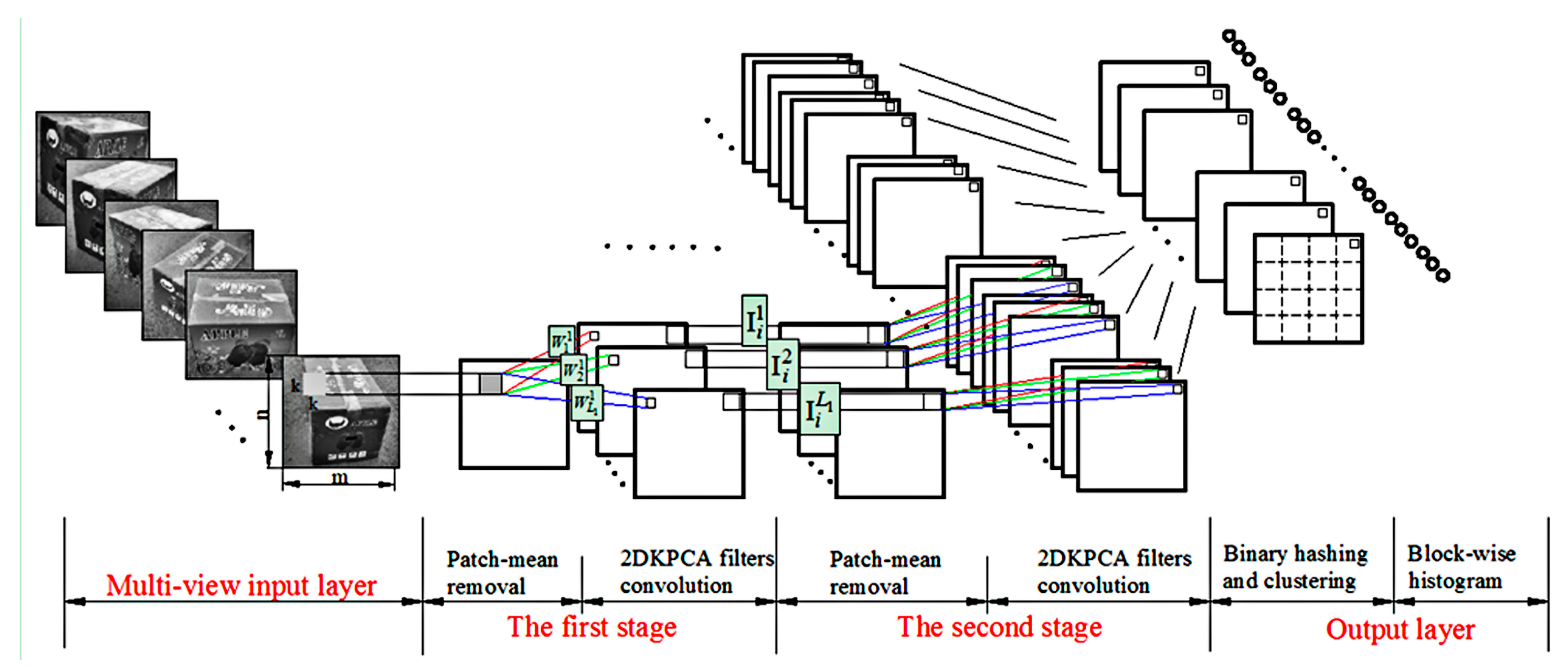
The BM2DKPCANet model for feature extraction of the input sequence images is divided into three stages. As shown in Figure 1, the output features are binary hashed and clustered after two-layer 2DKPCA convolutional filtering, followed by histogram features output.

The process of 2DKPCA convolutional filtering for the first filtering layer is described as follows. Suppose that there are S multi-view image sequences I_i (i = 1, 2, …, S) $\in$ R^{m × n} as samples for training. S local feature matrices T_i sized k² × mn are obtained after k × k windows for block sliding sampling. Then, the column direction kernel matrix dimension is Smn × Smn when performing centralized learning training. To reduce the computation, the average column vector is computed instead of the original column vector to obtain a nonlinear mapping sample ${\overline{T}}_i$, which is mapped to the kernel feature space as follow:

$${\Phi }_1=[\varphi ({\overline{T}}_1),\varphi ({\overline{T}}_2),\dots ,\varphi ({\overline{T}}_S)]$$

(1)

The kernel matrix can be expressed as:

$$K_1={\Phi }_1{}^T{\Phi }_1=[k({\overline{T}}_s,{\overline{T}}_s)]=[\langle \varphi ({\overline{T}}_s),\varphi ({\overline{T}}_s)\rangle ]$$

(2)

The dimensionality is reduced to S × S. The kernel matrix is centralized such that

$${\overline{K}}_1=K_1-\frac{1}{S}{K}_{1}1-\frac{1}{S}1K_1+\frac{1}{S^2}1K_{1}1$$

(3)

where 1 is the s-order matrix with all 1 components. The eigenvectors corresponding to the first L₁ largest eigenvalues are taken as 2DKPCA filter banks W_l¹ = [w₁, w₂,…, w_L1], which are convolved with the training sample I_i after the zero-filled boundary and then output the first-layer filtering:

$${{\rm I}}_i^l={{\rm I}}_i\ast W_l^1,i=1,2,\dots ,S;l=1,2,\dots ,L1$$

(4)

where $\ast$ is two-dimensional convolution.

It is also used as input for the second stage of convolutional filtering to further explore the effective classification features. The same steps as described previously are used to obtain the second stage filter set convolution kernel $W_{\ell }^2$ = [w₁, w₂, …, w_L2], The second layer filtering output is obtained by convolving the training samples ${{\rm I}}_i^l$ with the zero-padding boundary.

$$\begin{array}{l}{O}_i^l={{\rm I}}_i^l\ast W_{\ell }^2={{\rm I}}_i^{}\ast W_l^1\ast W_{\ell }^2,\\ s.t.i=1,2,\dots ,S;l=1,2,\dots ,L_1;\ell =1,2,\dots ,L_2\end{array}$$

(5)

In order to reduce the data redundancy caused in the process of multi-view image acquisition and reduce the computation time and storage space to solve problems such as large data storage and long-time operation of multiple views, the binary multi-view clustering algorithm [45] is used to optimize the binary encoding and cluster of multiple views jointly. The total optimization function is written as:

$$\begin{array}{l}\min F(U^{m^{\prime }},B^{\prime },C,G,\alpha )\\ ={\displaystyle {\sum }_{m^{\prime }=1}^M{({\alpha }^{m^{\prime }})}^r}({\Vert B^{\prime }-U^{m^{\prime }}\varphi (O^{l^{m^{\prime }}})\Vert }_F^2+\beta {\Vert U^{m^{\prime }}\Vert }_F^2\\ -\raisebox{1ex}{$\gamma $}\!\left/ \!\raisebox{-1ex}{$n^{\prime }$}\right.tr((U^{m^{\prime }}\varphi (O^{l^{m^{\prime }}})){(U^{m^{\prime }}\varphi (O^{l^{m^{\prime }}}))}^T)+\lambda {\Vert B^{\prime }-CG\Vert }_F^2\\ s.t.C^{T}1=0,{\displaystyle {\sum }_{m^{\prime }}{\alpha }^{m^{\prime }}=1},{\alpha }^{m^{\prime }}>0,B^{\prime }\in {\left\{-1,1\right\}}^{q^{\prime }\times n^{\prime }},\\ C\in {\left\{-1,1\right\}}^{q^{\prime }\times c},G\in {\left\{0,1\right\}}^{c\times n^{\prime }},{\displaystyle {\sum }_j{g}_j{}_i}=1.\end{array}$$

(6)

where ${\alpha }^{m^{\prime }}$ is the weight of the m^′th perspective of some fruit box, m^′ = 1, ..., M. Different perspectives have different weights. r > 1 is the scalar controlling the weight. $B^{\prime }=\left[b_1,\dots ,b_{n^{\prime }}\right]$, $b_i$ is the collaborative binary code for the ith instance. Each code b is represented by the product of clustering centroids C and indicator vector g. $U^{m^{\prime }}$ is the mapping matrix under the m^′th perspective. $\varphi ({\mathrm{O}}^{l^{m^{\prime }}})$ is the kernel function based on nonlinear RBF mapping of the output features after the second layer KPCA and randomly selected sample points from the m^′th perspective. $\gamma$ is a non-negative constant. $G=\left[g_1,\dots ,g_{n^{\prime }}\right]$ and $\lambda$ are the regularization parameters.

Each of the clustering characteristics after the above optimization is transformed into decimal:

$$T_i^{l^{m^{\prime }}}={\displaystyle {\sum }_{l=1}^{L_2}{2}^{l-1}}\left(h_i^{l^{m^{\prime }}}\right)$$

(7)

Each pixel of $T_i^{l^{m^{\prime }}}$($l\in [1,L_1]$) is an integer, and the range is $[0,2^{L_2-1}]$. Each $T_i^{l^{m^{\prime }}}$ is divided into Z blocks. For each block, histogram statistics are conducted. Full connection is taken to obtain:

$$f_i^{m^{\prime }}={[Zhist(T_i^{1^{m^{\prime }}}),\cdot \cdot \cdot ,Zhist(T_i^{L_1^{m^{\prime }}})]}^T\in {ℝ}^{(2^{L_2})L_{1}Z}$$

(8)

$f_i^{m^{\prime }}$ is the BM2DKPCANet feature of the ith sample from the m^′th perspective.

3. Optimal Path Planning for Multi-View Recognition Based on the A* Algorithm

3.1. Geometric Model for Target Observation

To search for the best path for accurate identification of multi-view targets, a geometry model for target observation is first built. Then, the best path search problem is transformed into a solving optimization problem.

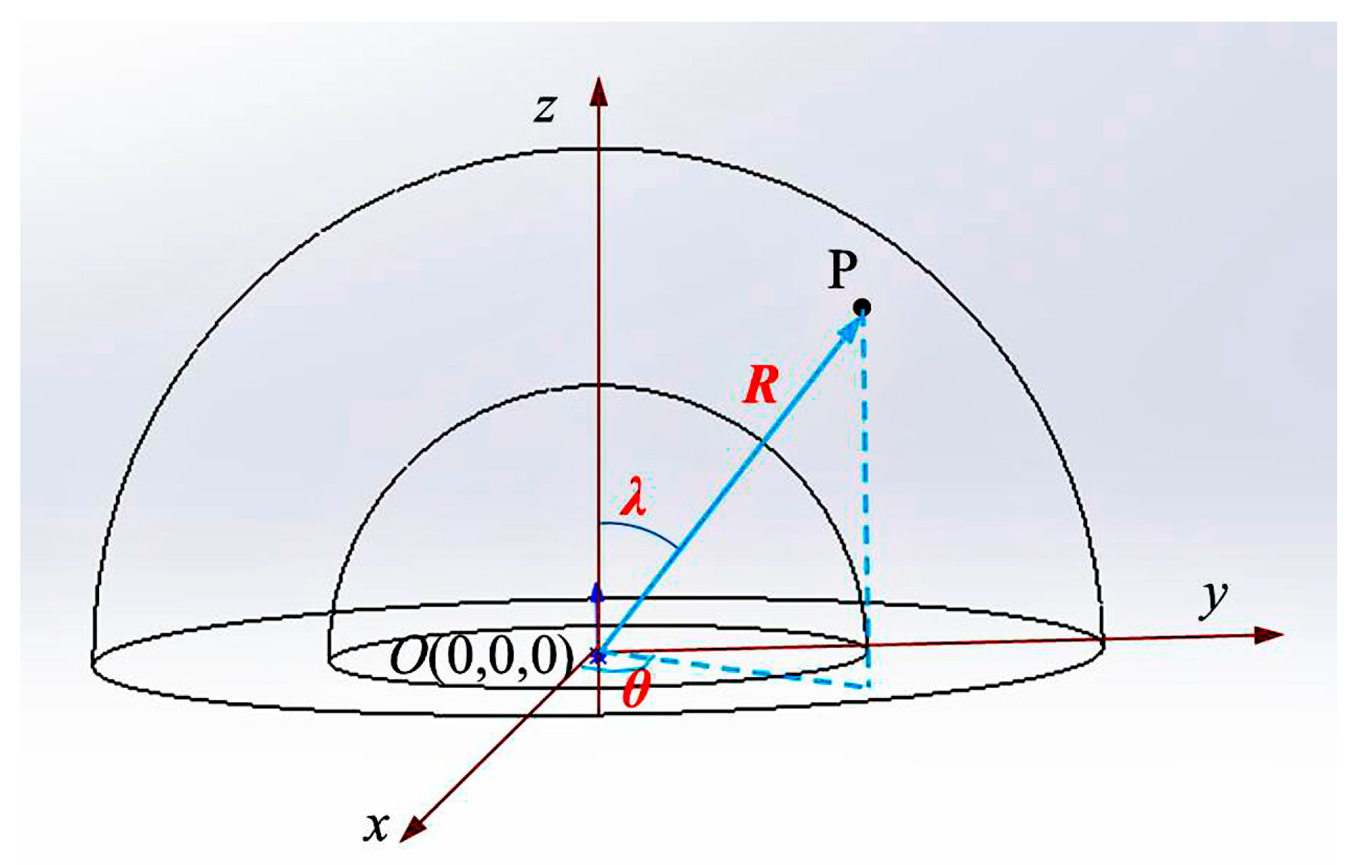
Within the working space of the robot arm, the observation geometry model is constructed as large as possible to obtain a better observation path. For meeting the requirements, an outer envelope sphere of the target is constructed. The radius range of the observation model is 3–5 times the radius of the outer envelope sphere. The hemispherical ring observation model shown in Figure 2 is constructed based on the target center position. The minimum and maximum observation circle radii of the observation area boundary are R_min and R_max, respectively. Suppose that the target centroid is located at the origin of coordinates O(0,0,0) and R is the distance of the camera viewpoint from the coordinate origin, that is, arc radius of perspective. Due to the specificity of the target observation model, a spherical coordinate system is used for position representation. Then, the viewpoint imaging coordinates of point P are denoted as P (R, λ, θ,), λ is the angle between the positive direction of z-axis and the directed line segment OP, 0 ≤ λ ≤ π/2, and θ (0 ≤ θ ≤ 2π) is the angle between the positive direction of the x-axis and the projection of the directed line segment OP on the xOy plane. The right-angle coordinate system is converted as:

$$\{\begin{array}{l}x=R\sin \lambda \cos \theta \\ y=R\sin \lambda \sin \theta \\ z=R\cos \lambda \end{array}$$

(9)

The conversion relation from a right-angle coordinate system to a spherical coordinate system is

$$\{\begin{array}{l}R=\sqrt{x^2+y^2+z^2}\\ \lambda =\arccos \frac{z}{R}\\ \theta =\arctan \frac{y}{x}\end{array}$$

(10)

The location of the optimal viewpoint is optimized by MHWOA, and the camera observation path passes through a series of imaging points and is planned as a polynomial function for interpolation to form a smooth curve. The camera observation path can be expressed as a sequence of coordinates as:

$${\mathrm{P}}_c=\left\{{\mathrm{P}}_1^v,{\mathrm{Q}}_1,{\mathrm{Q}}_2,\dots ,{\mathrm{Q}}_{n_1},{\mathrm{P}}_2^v,{\mathrm{Q}}_{n_1+1},{\mathrm{Q}}_{n_1+2},\dots ,{\mathrm{Q}}_{n_2},\dots ,{\mathrm{P}}_{k-1}^v,{\mathrm{Q}}_{n_{k-2}+1},\dots ,{\mathrm{Q}}_{n_{k-1}},{\mathrm{P}}_k^v\right\}$$

(11)

where ${\mathrm{P}}_p^v$ = (Rp, θp, λp), p = 1, 2, ..., k, are the coordinates of each imaging point, Q_q = (θ_q, λ_q, R_q) (q = 1, 2, …, n_k−1) are coordinates of the interpolation points between each imaging point.

The coordinate set of obstacles in the observation scene are set as B = {B1,B2,..., BE}, where Be = (Re, λe, Re), (e = 1, 2, ..., E) is the position coordinate of the eth surface obstacle. As one of the important measurement parameters, the influence range of obstacles on the path of manipulator can be expressed as parameter vector β (β₁, β₂, …, β_E).

The observation area is uniformly divided according to the latitude and longitude regions. Assuming that the longitude direction is uniformly divided into M_lo regions, and the dimensional direction is uniformly divided into M_la regions, then the observation model is divided into M_lo × M_la arc cone regions, and at most one imaging point is defined to exist in each arc region.

3.2. Objective Functions and Constraints

The path planning of viewpoints only needs to consider the shortest movement route and high efficiency of viewpoint recognition. The objective function of the mathematical model that transforms the viewpoint seeking path planning problem into a multi-objective optimization problem at this point can be expressed as:

$$\{\begin{array}{l}\max \stackrel{⌢}{R}(X)\\ \min \stackrel{⌢}{D}({\mathrm{P}}_c,{\mathrm{P}}_1)\end{array}$$

(12)

where the monotonically increasing function $\stackrel{⌢}{R}(X)$ represents the recognition performance of the multi-view target recognition system. The larger the function value is, the higher the recognition accuracy is. The information contained in the images obtained from different viewpoints at different locations is different, and the function $\stackrel{⌢}{R}(X)$ is also different. $\stackrel{⌢}{D}({\mathrm{P}}_c,{\mathrm{P}}_1)$ denotes the distance from the starting point P₁ of the observation path to the target point P_c.

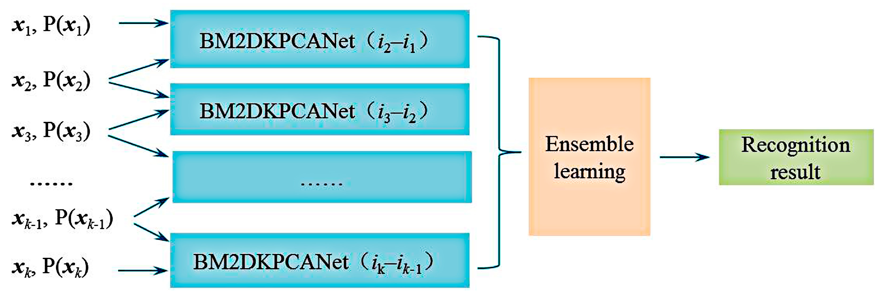
It is very difficult to find a specific analytic function to represent to characterize the recognition performance of the system theoretically. Based on the previous study of multi-view recognition of targets, this section selects the Softmax classifier for classification and outputs the category posterior probabilities to characterize the recognition performance. For more accurate identification, while the design of the classifier is further improved, combined with integrated learning theory, the single classifier is effectively combined, as shown in Figure 3 for the basic structure of BM2DKPCANet network-integrated multi-view classification. x_i is the original image acquired by the camera, and the imaging viewpoint of the pair of factors is P(x_i) = (R_p, θ_p, λ_p). The multi-viewpoint image is decomposed into image pairs and input to the two-viewpoint base classifier for classification and recognition, and then all the reco_gnition results are fused using an integrated learning method.

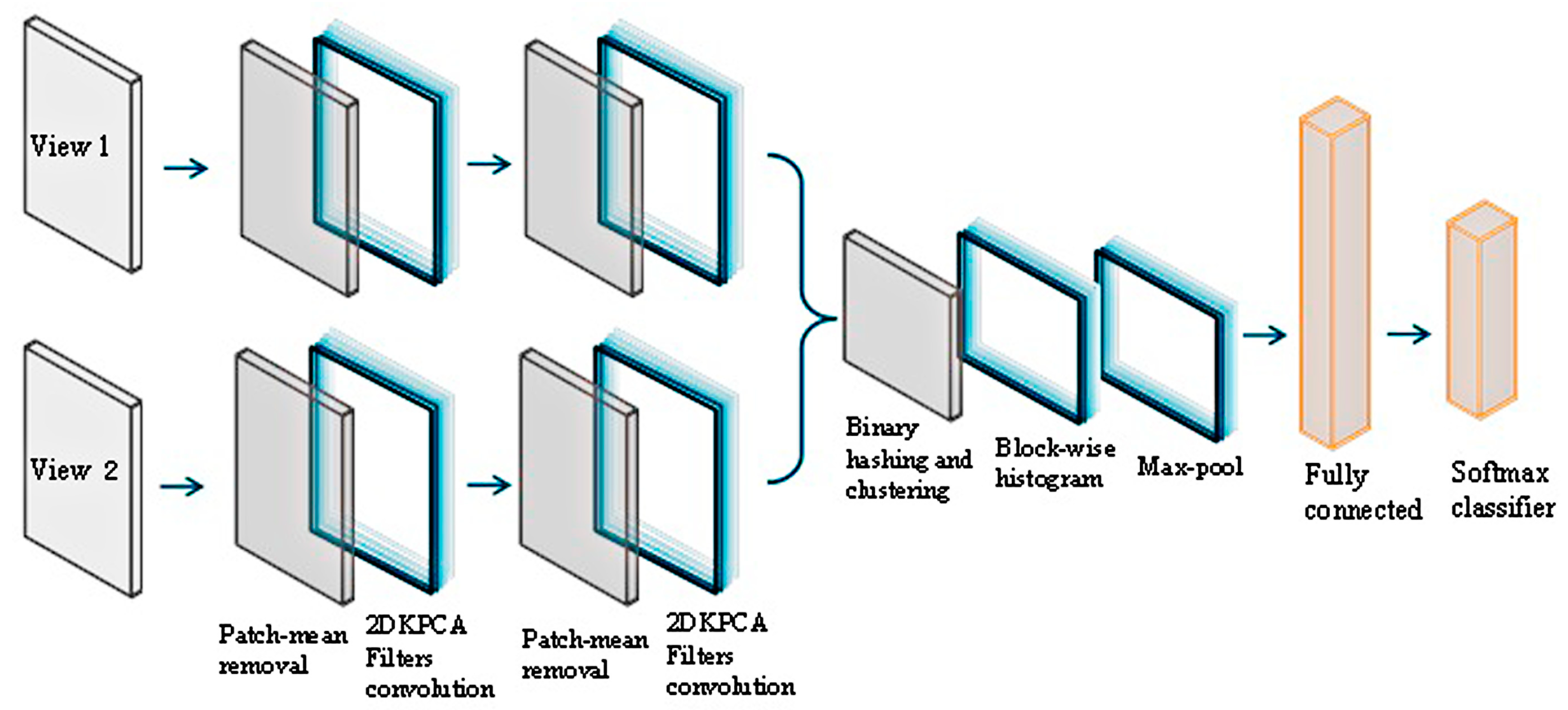
The structure of the two-view classifier network is shown in Figure 4. To better describe the recognition performance optimization function, the Softmax classifier is chosen to calculate the posterior probability to classify the image attributes.

In order to reduce the planning complexity and the number of divided intervals, this paper sets that the subsequent planning is carried out along the sphere with R as the radius when the viewpoint enters within the allowed boundary region, i.e., R is between R_l and R_u. According to the region division of the target observation model, the sphere is homogenized into M_lo·M_la regions, and the set of view intervals can be expressed as:

$$\begin{array}{l}\left\{({\theta }_i,{\lambda }_j)|{\theta }_i=\left[\frac{2\pi \cdot (i-1)}{{\mathrm{M}}_{la}},\frac{2\pi \cdot i}{{\mathrm{M}}_{la}}\right],{\lambda }_j=\left[\frac{\pi \cdot (i-1)}{2{\mathrm{M}}_{lo}},\frac{\pi \cdot i}{2{\mathrm{M}}_{lo}}\right]\right\}\\ s.t.i=1,2,\dots ,{\mathrm{M}}_{la},j=1,2,\dots ,{\mathrm{M}}_{lo}\end{array}$$

(13)

${\varphi }_{ij}$ is used to express the above perspective range. The set of perspective range can be further expressed as:

$$\left\{{\varphi }_{ij}|{\varphi }_{ij}=({\theta }_i,{\lambda }_j)\right\}$$

(14)

Each original image x_i belongs to only one of the view intervals. The classifier classifies only the image pairs within the viewpoint interval, and the original data set is reorganized into a series of image pairs as:

$$\left\{(x_u,x_v)|x_u\in X_i,x_v\in X_{i+d},\mathrm{P}(X_i)\in {\varphi }_{ij},\mathrm{P}(X_{i+d})\in {\varphi }_{(i+d_{\theta })(j+d_{\lambda })}\right\}$$

(15)

where d_θ is perspective interval difference in the dimensional direction and d_λ is perspective interval difference in longitude.

Some of these image pairs are randomly selected as training samples, and other image pairs are used as test samples to evaluate the recognition performance of the constructed BM2DKPCANet + Softmax classifier.

Based on the above approach, the final recognition results of the multi-view classifier after integrated learning can be expressed by the following equation:

$$\stackrel{⌢}{R}(x_1,x_2,\dots ,x_k)=\prod ({\displaystyle \sum _{i=1}^{k-1}{\mathbf{p}}_i(\mathbf{y}|x_i,x_{i+1})})$$

(16)

where {x₁, x₂, …, x_k} is a sequence of input multi-view images. $\prod (\cdot )$ is the index of the position of the maximum element of the input vector. p_i(y|x_i, x_i+1) is the C-dimensional posterior probability vector derived from the image classification by the base classifier, expressed as

$$p_i(y|x_i,x_i{}_{+1})=\left[\begin{array}{c}{p}_i(y_1|x_i,x_i{}_{+1})\\ p_i(y_2|x_i,x_i{}_{+1})\\ ⋮\\ \begin{array}{l}{p}_i(y_{C-1}|x_i,x_i{}_{+1})\\ p_i(y_C|x_i,x_i{}_{+1})\end{array}\end{array}\right]$$

(17)

where $p_i(y_h|x_i,x_i{}_{+1})$ (h = 1, 2,…,C) is the category posterior probability recognized of the input image by the basic classifier. It can be expressed as:

$$p_i(y_h|x_i,x_i{}_{+1})=p_i(y_h|z)=\frac{\exp (z_h)}{{\displaystyle \sum _{c=1}^C\exp (z_c)}}$$

(18)

where $z$ is the input of the classifier of the i-th identification network.

The constraint of viewpoint seeking path planning for robotic arms requires that the planned path points are in the target observation space, and also belong to the reachable workspace of the robotic arm. The difference in viewpoints between adjacent path points cannot exceed the number of base classifiers. The arm joint angles are within the joint limit angles. The speed, acceleration and pulse speed of each joint cannot exceed the corresponding maximum value. In summary, the mathematical model for transforming the viewpoint seeking path planning problem into a multi-objective optimization problem can be expressed as:

$$\begin{array}{l}\{\begin{array}{l}\max \stackrel{⌢}{R}(X)=\max (\stackrel{⌢}{R}({\mathrm{P}}_1^v,{\mathrm{P}}_2^v,\dots ,{\mathrm{P}}_k^v))=\max ({\displaystyle \sum R^{^\dot{d}}({\varphi }_{ij},{\varphi }_{(i+d_{\theta })(j+d_{\lambda })})})\\ \min \stackrel{⌢}{D}({\mathrm{P}}_c,{\mathrm{P}}_1)\end{array}\\ s.t.\{\begin{array}{l}\left\{{\mathrm{P}}_1^v,{\mathrm{P}}_2^v,\dots ,{\mathrm{P}}_k^v\right\}\in \mathsf{\Omega }\in \mathrm{W}\\ {\mathrm{P}}_f^v\in {\varphi }_{ij},{\mathrm{P}}_{f+1}^v\in {\varphi }_{(i+d_{\theta })(j+d_{\lambda })},f=1,2,\dots ,k-1,d_{\theta }\le {\mathrm{C}}_l,d_{\lambda }\le {\mathrm{C}}_l\\ {\theta }_s^d\le {\theta }_s\le {\theta }_s^u\\ |{\dot{\theta }}^s(t)|\le V_{\max }^s\\ |{\ddot{\theta }}^s(t)|\le A_{\max }^s\\ |{\stackrel{⃛}{\theta }}^s(t)|\le J_{\max }^s\end{array}\end{array}$$

(19)

where $\mathsf{\Omega }$ is the viewpoint position search space, W is the accessible workspace of the manipulator, ${\varphi }_{ij}$ is the range of view angle, $d_{\theta }$ is the view angle difference of latitude, $d_{\lambda }$ is the view angle difference of longitude, k is the number of view angles in path planning, ${\mathrm{C}}_l$ is the number of basic classifiers, ${\theta }_s$ is the joint angle of the sth joint, ${\theta }_s^d$ and ${\theta }_s^u$ are the upper and lower boundary of the angle movement for the sth joint, respectively. ${\dot{\theta }}^s(t)$, ${\ddot{\theta }}^s(t)$ and ${\stackrel{⃛}{\theta }}^s(t)$ are the actual velocity, acceleration and pulse of the sth joint of the manipulator at t time, respectively. $V_{\max }^s$, $A_{\max }^s$ and $J_{\max }^s$ are respectively the maximum velocity, maximum acceleration and maximum pulse of the sth joint of the manipulator.

3.3. Optimal Path Planning Based on A* Algorithm for Multi-View Recognition

This section abstracts the recognition performance distribution of the base classifier as a directed graph model for planning. The defined recognition rate of the base classifier for image pairs with inputs from the set of view intervals {${\varphi }_{ij}$, ${\varphi }_{(i+d_{\theta })(j+d_{\lambda })}$} is denoted as $R^{^}({\varphi }_{ij},{\varphi }_{(i+d_{\theta })(j+d_{\lambda })})$. The recognition performance directed graph model built when the number of base classifiers C_l = 3 is shown in Figure 5. The hemispherical view interval faces are expanded and displayed in the form of a plane, and the set of view intervals {${\varphi }_{11}$, ${\varphi }_{12}$, …, ${\varphi }_{1{\mathrm{M}}_{lo}}$,${\varphi }_{21}$,…, ${\varphi }_{{2\mathrm{M}}_{lo}}$,…, ${\varphi }_{{\mathrm{M}}_{la}1}$,…, ${\varphi }_{{\mathrm{M}}_{la}{\mathrm{M}}_{lo}}$} constitute the vertices of the directed graph. To avoid confusion, only the first row and the first column are shown in this figure; the remaining rows and columns are the same as the first row and the first column respectively. Angle interval difference is define as $\dot{d}$, and then $\dot{d}$ is set 1,2,3. The orange line represents the direction at $\dot{d}$ = 1, the blue curve represents the direction at $\dot{d}$ = 2, the purple curve represents the direction at $\dot{d}$ = 3, the green line represents the direction diagonally at $\dot{d}$ = 2, and the red line represents the direction diagonally at $\dot{d}$ = 3. The recognition rates of image pairs with different sets of view intervals $R^{^\dot{d}}({\varphi }_{ij},{\varphi }_{(i+d_{\theta })(j+d_{\lambda })})$ are the edge weights of the directed graph.

The adjacency matrix corresponding to the recognition accuracy of the directed graph is:

$$A_R=\left[\begin{array}{ccccccc}{A}_{11}& A_{12}& A_{13}& \cdots & A_{1({\mathrm{M}}_{la}-2)}& A_{1({\mathrm{M}}_{la}-1)}& A_{1{\mathrm{M}}_{la}}\\ A_{21}& A_{22}& A_{23}& \cdots & A_{2({\mathrm{M}}_{la}-2)}& A_{2({\mathrm{M}}_{la}-1)}& A_{2{\mathrm{M}}_{la}}\\ A_{31}& A_{32}& A_{33}& \cdots & A_{3({\mathrm{M}}_{la}-2)}& A_{3({\mathrm{M}}_{la}-1)}& A_{{3\mathrm{M}}_{la}}\\ ⋮& ⋮& ⋮& \ddots & ⋮& ⋮& ⋮\\ A_{({\mathrm{M}}_{la}-2)1}& A_{({\mathrm{M}}_{la}-2)2}& A_{({\mathrm{M}}_{la}-2)3}& \cdots & A_{({\mathrm{M}}_{la}-2)({\mathrm{M}}_{la}-2)}& A_{({\mathrm{M}}_{la}-2)({\mathrm{M}}_{la}-1)}& A_{({\mathrm{M}}_{la}-2){\mathrm{M}}_{la}}\\ A_{({\mathrm{M}}_{la}-1)1}& A_{({\mathrm{M}}_{la}-1)2}& A_{({\mathrm{M}}_{la}-1)3}& \cdots & A_{({\mathrm{M}}_{la}-1)({\mathrm{M}}_{la}-2)}& A_{({\mathrm{M}}_{la}-1)({\mathrm{M}}_{la}-1)}& A_{({\mathrm{M}}_{la}-1){\mathrm{M}}_{la}}\\ A_{{\mathrm{M}}_{la}1}& A_{{\mathrm{M}}_{la}2}& A_{{\mathrm{M}}_{la}3}& \cdots & A_{{\mathrm{M}}_{la}({\mathrm{M}}_{la}-2)}& A_{{\mathrm{M}}_{la}({\mathrm{M}}_{la}-1)}& A_{{\mathrm{M}}_{la}{\mathrm{M}}_{la}}\end{array}\right]$$

(20)

where $A_R\in {ℝ}^{{\mathrm{M}}_{lo}{\mathrm{M}}_{la}\times {\mathrm{M}}_{lo}{\mathrm{M}}_{la}}$, $A_{ij}\in {ℝ}^{{\mathrm{M}}_{lo}\times {\mathrm{M}}_{lo}}$.

When i = j, the matrix A_ij = A_ii is shown in Equation (21). C_l is defined as the number of basic classifiers. $\dot{d}$ = 1,2..., Cl. When j = i + $\dot{d}$ ≤ M_la, the specific elements of matrix A_ij = A_{i(i+ $\dot{d}$)} is shown in Equation (22). When i ≥ M_la − $\dot{d}$ + 1 and j = i + $\dot{d}$ − M_la, the specific elements of matrix A_ij = $A_{i(i+\dot{d}-M_{la})}$ are shown in Equation (23). A_ij of the other cases is the 0 matrix f M_lo × M_lo.

$$A_{ii}=\left[\begin{array}{cccccccc}0& R_{[i1,i2]}^{^1}& R_{[i1,i3]}^{^2}& \cdots & R_{[i1,i(1+\dot{d})]}^{^\dot{d}}& 0& \cdots & 0\\ 0& 0& R_{[i2,i3]}^{^1}& R_{[i2,i4]}^{^2}& \cdots & R_{[i2,i(2+\dot{d})]}^{^\dot{d}}& 0& \cdots \\ 0& 0& 0& R_{[i3,i4]}^{^1}& R_{[i3,i5]}^{^2}& \cdots & 0& \cdots \\ ⋮& ⋮& ⋮& ⋮& ⋮& ⋮& ⋮& ⋮\\ 0& 0& 0& 0& R_{[i(M_{lo}-\dot{d}),i(M_{lo}-\dot{d}+1)]}^{^1}& \cdots & R_{[i(M_{lo}-\dot{d}),i(M_{lo}-1)]}^{^\dot{d}-1}& R_{[i(M_{lo}-\dot{d}),i{M}_{lo}]}^{^\dot{d}}\\ 0& 0& 0& 0& 0& R_{[i(M_{lo}-\dot{d}+1),i(M_{lo}-\dot{d}+2)]}^{^1}& \cdots & R_{[i(M_{lo}-\dot{d}+1),i{M}_{lo}]}^{^\dot{d}-1}\\ ⋮& ⋮& ⋮& ⋮& ⋮& ⋮& ⋮& ⋮\\ 0& 0& 0& 0& 0& 0& 0& R_{[i(M_{lo}-1),i{M}_{lo}]}^{^1}\\ 0& 0& 0& 0& 0& 0& 0& 0\end{array}\right]$$

(21)

$$A_{i(i+\dot{d})}=\left[\begin{array}{ccccccccc}{R}_{[i1,(i+\dot{d})1]}^{^\dot{d}}& 0& \cdots & 0& R_{[i1,(i+\dot{d})(1+\dot{d})]}^{^\dot{d}}& 0& 0& \cdots & 0\\ 0& R_{[i2,(i+\dot{d})2]}^{^\dot{d}}& 0& \cdots & 0& R_{[i2,(i+\dot{d})(2+\dot{d})]}^{^\dot{d}}& 0& \cdots & 0\\ 0& 0& R_{[i3,(i+\dot{d})3]}^{^\dot{d}}& 0& \cdots & 0& R_{[i3,(i+\dot{d})(3+\dot{d})]}^{^\dot{d}}& 0& \cdots \\ ⋮& ⋮& ⋮& ⋮& ⋮& ⋮& ⋮& ⋮& ⋮\\ 0& 0& 0& 0& R_{[i(M_{lo}-\dot{d}),(i+\dot{d})(M_{lo}-\dot{d})]}^{^\dot{d}}& 0& \cdots & 0& R_{[i(M_{lo}-\dot{d}),(i+\dot{d})M_{lo}]}^{^\dot{d}}\\ 0& 0& 0& 0& 0& R_{[i(M_{lo}-\dot{d}+1),(i+\dot{d})(M_{lo}-\dot{d}+1)]}^{^\dot{d}}& 0& \cdots & 0\\ 0& 0& 0& 0& 0& 0& R_{[i(M_{lo}-\dot{d}+2),(i+\dot{d})(M_{lo}-\dot{d}+2)]}^{^\dot{d}}& \cdots & 0\\ ⋮& ⋮& ⋮& ⋮& ⋮& ⋮& ⋮& ⋮& ⋮\\ 0& 0& 0& 0& 0& 0& 0& 0& R_{[i{M}_{lo},(i+\dot{d})M_{lo}]}^{^\dot{d}}\end{array}\right]$$

(22)

$$A_{i(i+\dot{d}-M_{la})}=\left[\begin{array}{ccccccccc}{R}_{[i1,(i+\dot{d}-M_{la})1]}^{^\dot{d}}& 0& \cdots & 0& R_{[i1,(i+\dot{d}-M_{la})(1+\dot{d})]}^{^\dot{d}}& 0& 0& \cdots & 0\\ 0& R_{[i2,(i+\dot{d}-M_{la})2]}^{^\dot{d}}& 0& \cdots & 0& R_{[i2,(i+\dot{d}-M_{la})(2+\dot{d})]}^{^\dot{d}}& 0& \cdots & 0\\ 0& 0& R_{[i3,(i+\dot{d}-M_{la})3]}^{^\dot{d}}& 0& \cdots & 0& R_{[i3,(i+\dot{d}-M_{la})(3+\dot{d})]}^{^\dot{d}}& 0& \cdots \\ ⋮& ⋮& ⋮& ⋮& ⋮& ⋮& ⋮& ⋮& ⋮\\ 0& 0& 0& 0& R_{[i(M_{lo}-\dot{d}),(i+\dot{d}-M_{la})(M_{lo}-\dot{d})]}^{^\dot{d}}& 0& \cdots & 0& R_{[i(M_{lo}-\dot{d}),(i+\dot{d}-M_{la})M_{lo}]}^{^\dot{d}}\\ 0& 0& 0& 0& 0& R_{[i(M_{lo}-\dot{d}+1),(i+\dot{d}-M_{la})(M_{lo}-\dot{d}+1)]}^{^\dot{d}}& 0& \cdots & 0\\ 0& 0& 0& 0& 0& 0& R_{[i(M_{lo}-\dot{d}+2),(i+\dot{d}-M_{la})(M_{lo}-\dot{d}+2)]}^{^\dot{d}}& \cdots & 0\\ ⋮& ⋮& ⋮& ⋮& ⋮& ⋮& ⋮& ⋮& ⋮\\ 0& 0& 0& 0& 0& 0& 0& 0& R_{[i{M}_{lo},(i+\dot{d}-M_{la})M_{lo}]}^{^\dot{d}}\end{array}\right]$$

(23)

Given the starting imaging point, the multi-view target viewpoint optimization path planning in barrier-free environment is equivalent to the directed graph path search problem with a given starting point. The number of nodes to be searched is k − 1, and the maximum path corresponding to the sum of edge weights is the search path. In order to facilitate the graph search, the problem of maximizing the sum of edge weights is transformed into the problem of minimizing the sum of search path weights by finding the reciprocal and normalized to (0,1):

$$R_e({\varphi }_{ij},{\varphi }_{(i+d_{\theta })(j+d_{\lambda })})=\frac{\frac{1}{R^{^}({\varphi }_{ij},{\varphi }_{(i+d_{\theta })(j+d_{\lambda })})}-R_{e\min }^{^}}{R_{e\max }^{^}-R_{e\min }^{^}}+\epsilon$$

(24)

where $R_{e\max }^{^}$,$R_{e\min }^{^}$ are the maximum and minimum values of the reciprocal of edge weights, respectively. ε is the parameter to ensure the continuity of directed edges.

The transformed matrix R_e becomes a new recognition performance matrix. In addition to recognition performance, it also ensures the shortest end running distance to improve operation efficiency. When the end enters the set observation radius range, the fixed radius does not move, and the path planning is carried out on the semicircular sphere with this radius as the radius. Similarly, viewpoint intervals are set as the vertexes of the directed graph, and the distances between two viewpoints are defined as the edge weights of the directed graph. The adjacency matrix D_R is constructed, which can be expressed as:

$$D_R=\left[\begin{array}{ccccccc}{D}_{11}& D_{12}& D_{13}& \cdots & D_{1({\mathrm{M}}_{la}-2)}& D_{1({\mathrm{M}}_{la}-1)}& D_{1{\mathrm{M}}_{la}}\\ D_{21}& D_{22}& D_{23}& \cdots & D_{2({\mathrm{M}}_{la}-2)}& D_{2({\mathrm{M}}_{la}-1)}& D_{2{\mathrm{M}}_{la}}\\ D_{31}& D_{32}& D_{33}& \cdots & D_{3({\mathrm{M}}_{la}-2)}& D_{3({\mathrm{M}}_{la}-1)}& D_{{3\mathrm{M}}_{la}}\\ ⋮& ⋮& ⋮& \ddots & ⋮& ⋮& ⋮\\ D_{({\mathrm{M}}_{la}-2)1}& D_{({\mathrm{M}}_{la}-2)2}& D_{({\mathrm{M}}_{la}-2)3}& \cdots & D_{({\mathrm{M}}_{la}-2)({\mathrm{M}}_{la}-2)}& D_{({\mathrm{M}}_{la}-2)({\mathrm{M}}_{la}-1)}& D_{({\mathrm{M}}_{la}-2){\mathrm{M}}_{la}}\\ D_{({\mathrm{M}}_{la}-1)1}& D_{({\mathrm{M}}_{la}-1)2}& D_{({\mathrm{M}}_{la}-1)3}& \cdots & D_{({\mathrm{M}}_{la}-1)({\mathrm{M}}_{la}-2)}& D_{({\mathrm{M}}_{la}-1)({\mathrm{M}}_{la}-1)}& D_{({\mathrm{M}}_{la}-1){\mathrm{M}}_{la}}\\ D_{{\mathrm{M}}_{la}1}& D_{{\mathrm{M}}_{la}2}& D_{{\mathrm{M}}_{la}3}& \cdots & D_{{\mathrm{M}}_{la}({\mathrm{M}}_{la}-2)}& D_{{\mathrm{M}}_{la}({\mathrm{M}}_{la}-1)}& D_{{\mathrm{M}}_{la}{\mathrm{M}}_{la}}\end{array}\right]$$

(25)

where $D_R\in {ℝ}^{{\mathrm{M}}_{lo}{\mathrm{M}}_{la}\times {\mathrm{M}}_{lo}{\mathrm{M}}_{la}}$,$D_{ij}\in {ℝ}^{{\mathrm{M}}_{lo}\times {\mathrm{M}}_{lo}}$, i = 1,2,…,M_la, j = 1,2,…,M_la.

When i = j, the specific elements of D_ij = D_ii are shown in Equation (26). $\dot{d}$ = 1, 2, …, C_l, 0 < r^{^1} < r^{^2} < ...< r^{^$\dot{d}$} ≤ 1 are the normalized weight set proportional to the distance between viewpoints.

$$D_{ii}=\left[\begin{array}{cccccccc}0& r^{^1}& r^{^2}& \cdots & r^{^\dot{d}}& 0& \cdots & 0\\ 0& 0& r^{^1}& r^{^2}& \cdots & r^{^\dot{d}}& 0& \cdots \\ 0& 0& 0& r^{^1}& r^{^2}& \cdots & 0& \cdots \\ ⋮& ⋮& ⋮& ⋮& ⋮& ⋮& ⋮& ⋮\\ 0& 0& 0& 0& r^{^1}& \cdots & r^{^(\dot{d}-1)}& r^{^\dot{d}}\\ 0& 0& 0& 0& 0& r^{^1}& \cdots & r^{^(\dot{d}-1)}\\ ⋮& ⋮& ⋮& ⋮& ⋮& ⋮& ⋮& ⋮\\ 0& 0& 0& 0& 0& 0& 0& r^{^1}\\ 0& 0& 0& 0& 0& 0& 0& 0\end{array}\right]$$

(26)

When j = i + $\dot{d}$ ≤ M_la, matrix D_ij = D_{i(i+ $\dot{d}$)}, specific elements are listed in Equation (27). When i ≥ M_la − $\dot{d}$ + 1 and j = i + $\dot{d}$ − M_la, specific elements of matrix $D_{i(i+\dot{d}-M_{la})}$ are listed in Equation (27). The difference of two non-0 elements in each row is $\dot{d}$ columns. D_ij of the other cases are M_lo × M_lo 0 matrix.

$$D_{i(i+\dot{d})}=D_{i(i+\dot{d}-M_{la})}=\left[\begin{array}{ccccccccc}{r}^{^\dot{d}}& 0& \cdots & 0& r^{^\dot{d}}& 0& 0& \cdots & 0\\ 0& r^{^\dot{d}}& 0& \cdots & 0& r^{^\dot{d}}& 0& \cdots & 0\\ 0& 0& r^{^\dot{d}}& 0& \cdots & 0& r^{^\dot{d}}& 0& \cdots \\ ⋮& ⋮& ⋮& ⋮& ⋮& ⋮& ⋮& ⋮& ⋮\\ 0& 0& 0& 0& r^{^\dot{d}}& 0& \cdots & 0& r^{^\dot{d}}\\ 0& 0& 0& 0& 0& r^{^\dot{d}}& 0& \cdots & 0\\ 0& 0& 0& 0& 0& 0& r^{^\dot{d}}& \cdots & 0\\ ⋮& ⋮& ⋮& ⋮& ⋮& ⋮& ⋮& ⋮& ⋮\\ 0& 0& 0& 0& 0& 0& 0& 0& r^{^\dot{d}}\end{array}\right]$$

(27)

Considering the two optimization problems of optimal recognition performance and shortest planning path, based on the same directed graph model, the weight ω is introduced to adjust the recognition performance and planning path distance to further transform the problem into a single optimization problem, which is the shortest path search on the directed graph. The directed graph is defined as G = (ϕ_ij,A), then the fused adjacency matrix can be expressed as:

$$A=\omega \cdot R_e+(1-\omega )D_R$$

(28)

As a typical heuristic search algorithm in artificial intelligence, the A* algorithm has been widely used in path solving. The algorithm introduces the path evaluation formula when selecting nodes:

$$f(n)=g(n)+h(n)$$

(29)

where g(n) is actual cost from initial state to state n, h(n) is the estimation cost of the optimal path from the state n to the target state.

In this section, the A* algorithm is used to solve the single-source shortest path problem of the fused directed graph, and the sum of the edge weights of the fused directed graph is defined as the cost function to complete the viewpoint optimization path planning in a barrier-free environment. The specific search process is shown in Figure 6. The A* algorithm uses two lists of openList and closeList to place the nodes to be examined and the nodes that have been examined, and sets the subsequent node table to store the subsequent nodes. Through the above operations, k viewpoints with the minimum sum of edge weights in P can be obtained. However, since the path searched by the A* algorithm is a spatial straight-line segment, in order to prevent the jitter and vibration of the manipulator during operation, the B-spline curve is used for interpolation and smoothing between the viewpoints of the end path to obtain the continuous and stable optimal observation path of the target, and the target recognition results are obtained through the classifier mentioned above.

4. Experimental Verification and Analysis

4.1. Construction of Experimental Platform

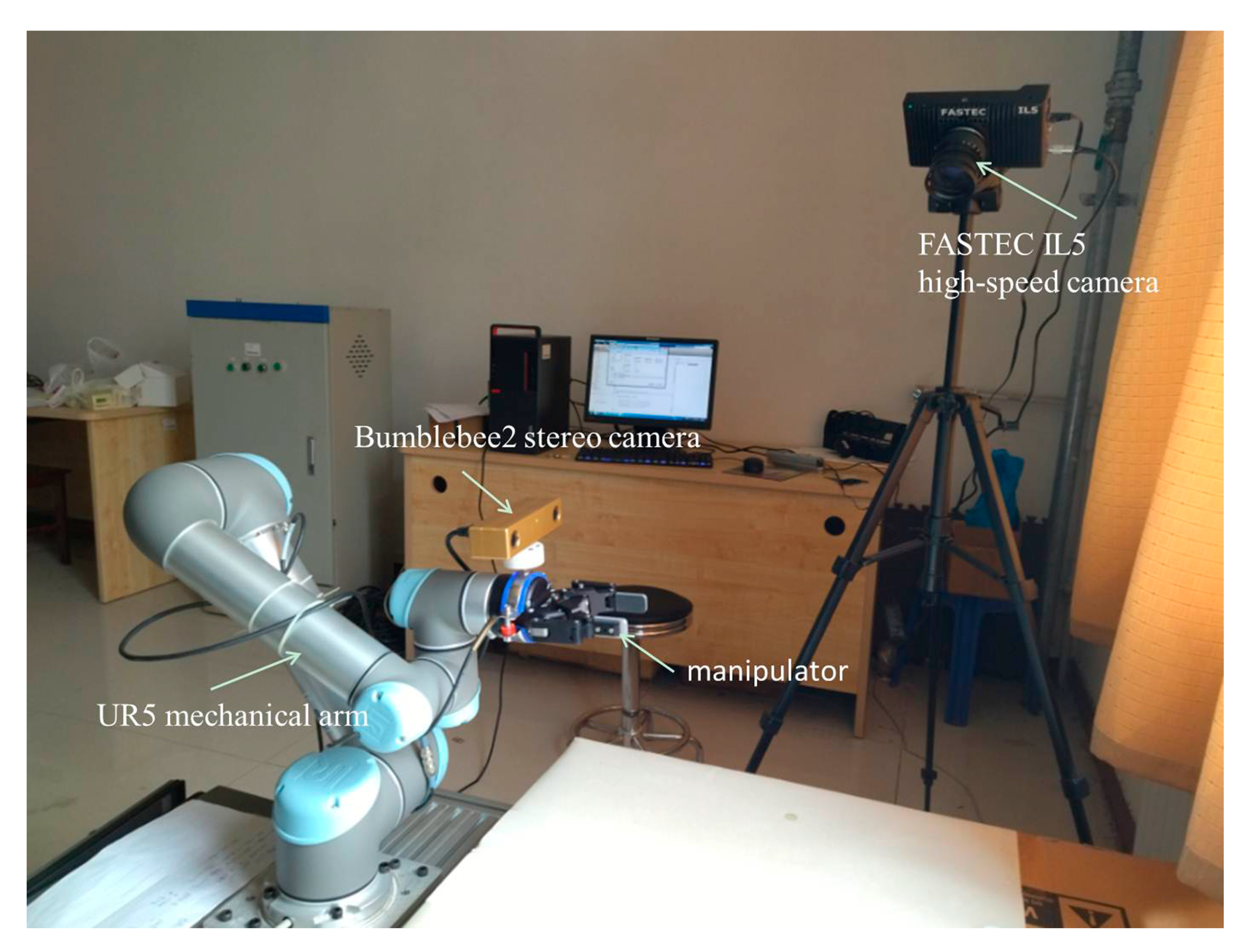
The experimental platform include the UR5 six degree of freedom industrial robot developed by Universal Robots, the stereo vision Bumblebee2 binocular camera developed by Point Grey Research of Canada, the Fastec IL5 high-speed camera, the 2F-85 ROBOTIQ double finger electric gripper, the image acquisition card matching the UR5 robot, etc., which are shown in Figure 7.

UR5 manipulator is a cooperative manipulator with small shape, simple programming, flexible action and safe use. It can complete loading, unloading, sorting, assembly and other work in production. Its effective load is 5 ± 0.5 kg, the maximum working range can reach the sphere space with 850 mm radius, the motion range of each joint is (−2π, 2π), and the maximum motion speed is 180°/s. Two kinds of cameras are used in this experiment. Fastec IL5 high-speed camera is fixed and used as a global camera for monitoring. Combined with the experimental content, it will not be introduced here. The Bumblebee2 binocular camera is fixed at the end of the manipulator to obtain the local features of the target and the depth information of the point cloud, and complete the viewpoint optimization path.

4.2. Camera Calibration and Motion Control

4.2.1. Camera Calibration

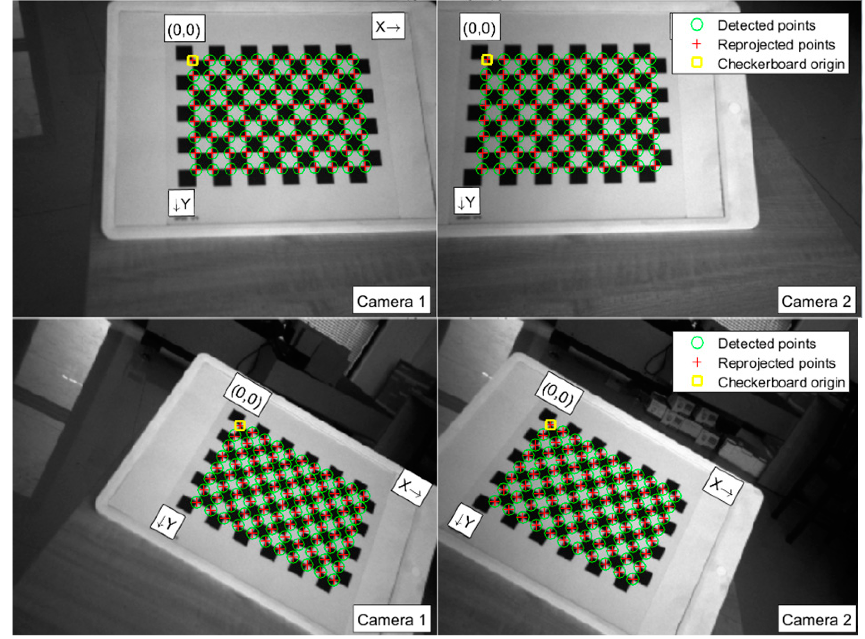
The binocular camera is connected to the end of the manipulator by a fixed clip to ensure that there is no relative motion between the manipulator and the camera during the motion. The calibration plate is fixed in front of the manipulator to calibrate the ‘eye on hand’. Under the premise of ensuring that the left and right cameras can observe a complete chessboard, the manipulator is controlled to reach 25 different poses, and the images are collected. The images collected by the left and right cameras are saved respectively, and calibrated based on Matlab. Some calibration results are shown in Figure 8. After removing the image pairs with large errors in the calibration process, the average calibration error is 0.15 pixels. Camera parameters are then exported. The internal parameter matrix of camera 1 is:

$$M_1=\left[\begin{array}{ccc}661.1927& 0& 258.8510\\ 0& 660.7811& 196.0307\\ 0& 0& 1\end{array}\right]$$

(30)

Its radial distortion parameter K1 = 0.0325, K2 = −0.0619. Tangential distortion parameters P1 and P2 are 0. The internal parameter matrix of camera 2 is:

$$M_2=\left[\begin{array}{ccc}661.8001& 0& 249.2579\\ 0& 661.1257& 196.2485\\ 0& 0& 1\end{array}\right]$$

(31)

Its radial distortion parameters K1 = 0.0203 and K2 = −0.0815. Tangential distortion parameters P1 and P2 are 0.

4.2.2. Control of Manipulator

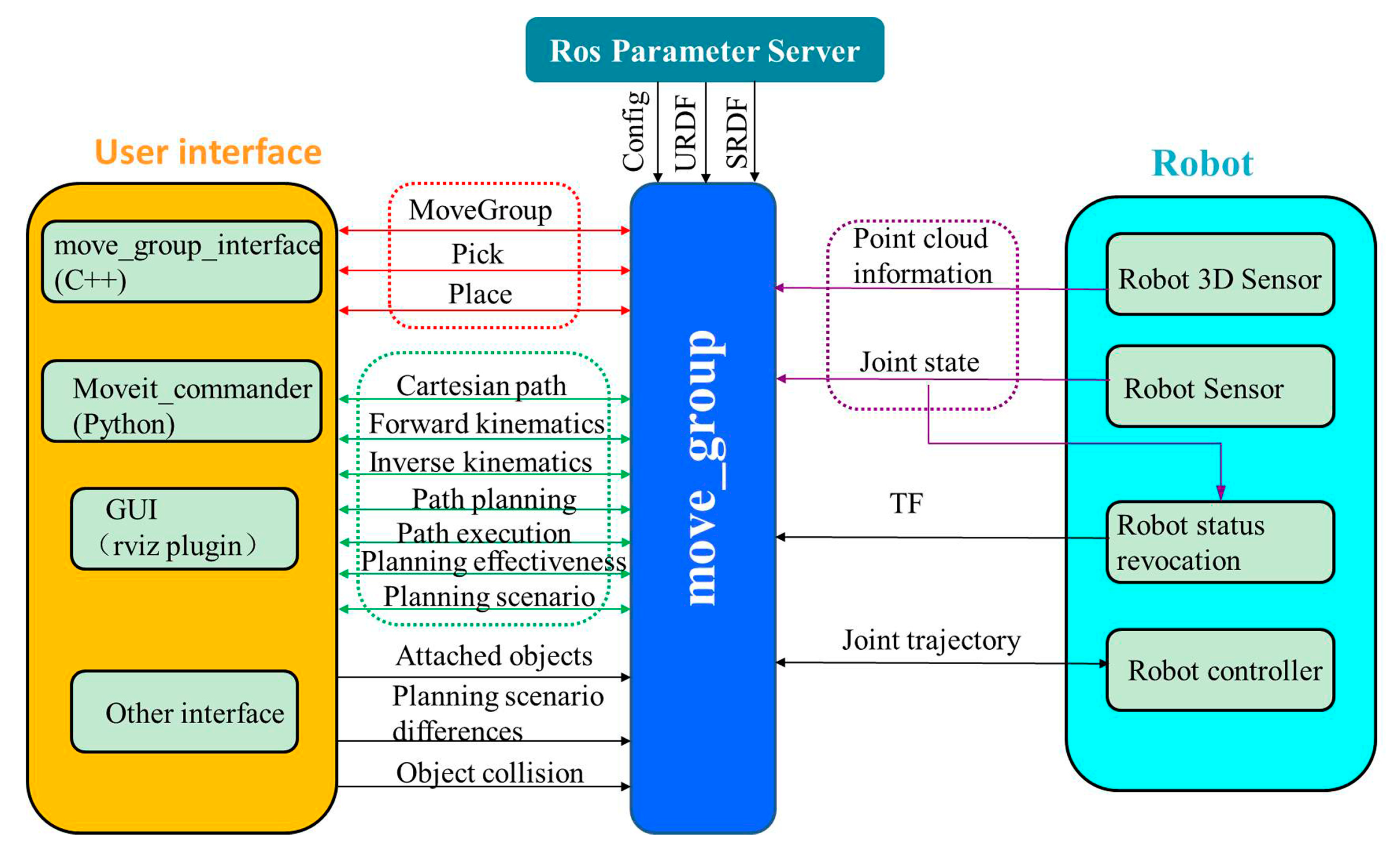
The UR5 manipulator is controlled based on the ROS system in Linux environment. The system includes motion planning, 3D perception and other functional modules. The MoveIt! module for manipulator controlling can realize modeling, kinematics calculation, path obstacle avoidance planning, etc. The structure is shown in Figure 9. The core node is move_group, which connect to plug-ins to implement various functions. The Ubuntu version used in this experiment is 16.04, and the ROS version is Kinetic. The used toolkits are listed as follows. The ros_kinetic_ur_description contains the model information of UR series robots. The ur5_ros_controllers are connected with the robot hardware interface to obtain the robot information data in real time, which are sent to the manipulator driving part for path planning. The ROS Param Server is a parameter server which is used to define setting parameters, model files and configuration files. The Robot 3D sensors can obtain the image data from the camera, which are used to identify location, positioning, grasping, obstacle avoidance, etc. The User interface provides a series of API for function customization. The ur_ros_ sensors can obtain the sensor data of the manipulator and calculate the motion state of the robot.

4.3. Optimization Path Planning for Multi-View Recognition

In order to test the performance of the proposed multi-view target optimal view path planning method in barrier free environment, this section takes the medicine box as the recognition object and generates the training set and verification set. Different starting points and different numbers of view angles are set to verify.

4.3.1. Path Planning with Different Perspectives

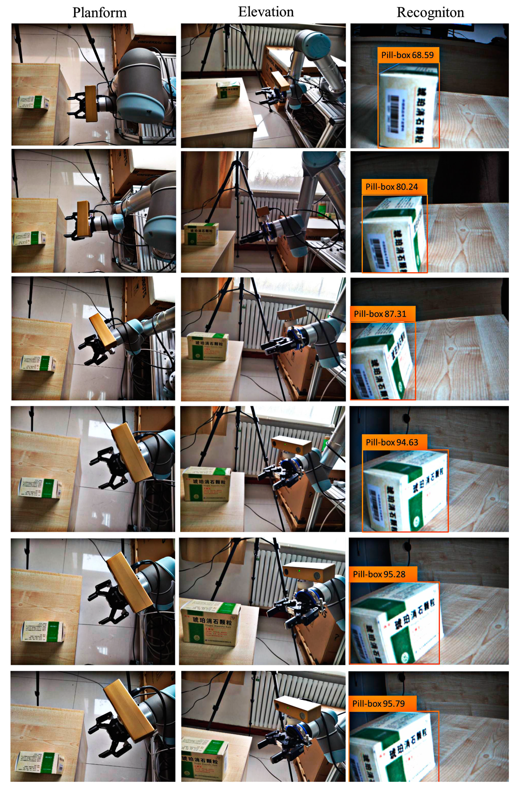
The viewing angle interval is divided into 36 parts in the latitude direction and nine parts in the longitude direction. The number of divided viewing angle intervals of the target observation model is 324. The images of the medicine box are collected, the data set corresponding to the viewing angle interval ϕ_ij(i = 1, 2, …, 36; j = 1, 2, …, 9) is reorganized, obtaining 324 groups of data. There are 15 original images in each group of data, and any two groups of data can generate 15 × 15 image pairs, which are used for classification training and verification of basic classifiers. Set the number of basic classifiers C_l = 3. The input image size is 128 × 128. The sampling block size is 5 × 5. The size of histogram block is 8 × 8. The block overlap rate is 0.5. Gaussian kernel function is selected. In adjacency matrix D_i, d^¹ = 0.3, d^² = 0.6, d^³ = 1, ω = 0.5, ε = 1 × 10⁻⁶. Firstly, the starting point is set to interval ϕ₁₁, and the number of viewing angles k = 3, 4, 5 are taken respectively. The observed viewpoint optimization path is shown in Figure 10.

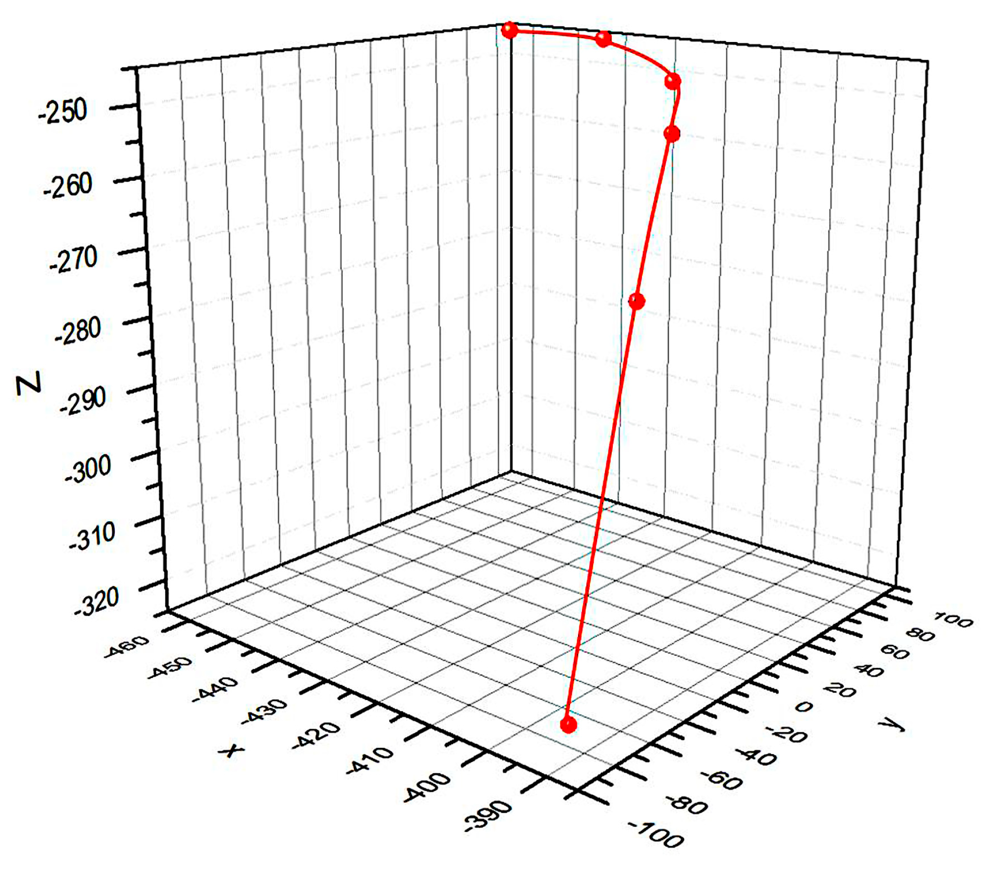
Figure 10 lists the top view, front view and camera recognition view that can characterize the position relationship with the target object at different viewpoints in path planning. The first line is the starting viewpoint. When the number of viewing angles is selected as three, the planned camera will reach the position of lines 2, 3 and 4 from the position of line 1 one by one. Similarly, increasing the number of viewing angles, the manipulator adds the planning to the position of line 5 and line 6. According to the image recognition results, when the number of viewing angles is three, the recognition accuracy has reached 94.63%. Increasing the number of viewing angles, although the recognition accuracy has increased, it has little change. When the number of viewing angles is 5, the planned path is shown in Figure 11. It can be seen that the initial path is mainly the elevation in the Z-axis direction, and then move in the X-axis and Y-axis. The target is observed in multiple directions to improve the recognition accuracy.

4.3.2. Path Planning with Different Starting Points

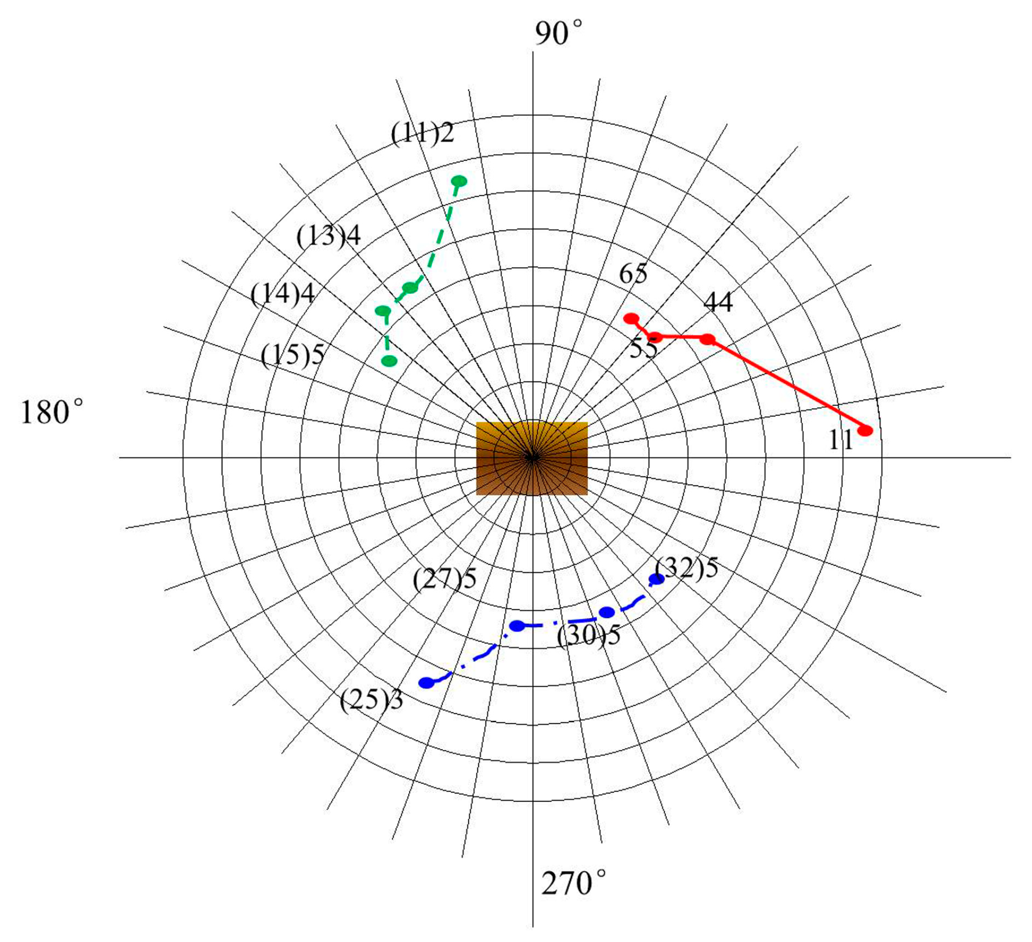
Different starting points are selected to determine the optimal viewpoint path planning. The top views of the observation models are shown in Figure 12, Figure 13 and Figure 14. Figure 12 shows the optimal path when the number of viewing angles is three. The starting point of the red real line track is ϕ₁₁, the starting point of the green dotted line track is ϕ₍₁₁₎₂, and the starting point of the blue dotted line track is ϕ₍₂₅₎₃.

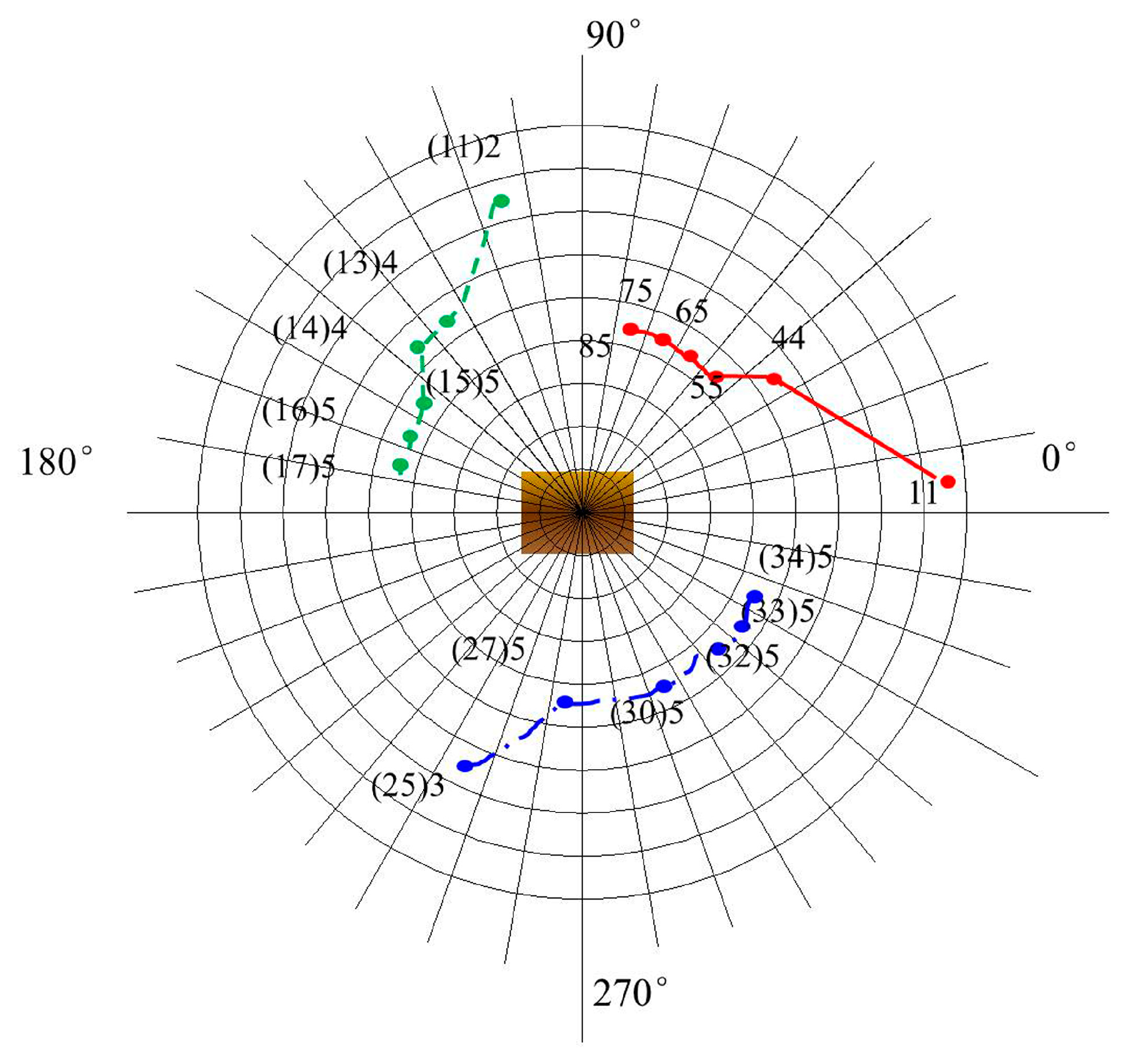
Figure 13 is the optimal path with viewing angles = 4, Figure 14 is the optimal path with viewing angles = 5, and the color and track starting point is consistent with Figure 12. By comparing the three figures, it can be seen that the planned path can quickly reach the better viewing point. With the bottom as the benchmark, the longitude direction is about 50°, and then the trend is mainly planned along the latitude direction. When the angle of view is 3, the path planning can complete the identification of two sides and top surfaces. Increasing the viewpoint angles, the movement is mainly along the latitude direction. It can be concluded that this method can well complete the viewpoint optimization path planning under different starting points and different viewing angle constraints in the barrier free environment, and effectively complete the optimal balance between recognition performance and search speed.

The performance of target recognition is compared with different starting viewpoints and different viewing angles. When the number of viewing angles is 3, the recognition accuracy of different starting viewpoints is shown in

Table 1. Recognition with different starting points with 3 viewing angles.

	Longitude	1	2	3	4	5	6	7	8	9
Latitude
1		95.82	96.35	96.47	96.38	96.27	95.28	89.21	85.07	84.24
2		96.04	96.28	96.34	96.56	96.48	96.03	90.24	86.07	84.56
3		96.59	96.64	96.69	96.78	96.71	95.86	91.2	84.32	83.74
4		96.21	96.33	96.48	96.52	96.54	95.29	93.21	85.14	83.22
5		90.28	91.97	91.98	91.55	91.49	89.23	87.42	83.21	82.89
6		90.37	90.58	91.24	91.28	90.97	89.86	88.47	82.89	82.67
7		91.58	92.48	92.77	92.64	92.85	91.87	87.65	83.11	82.9
8		94.05	94.62	94.77	96.58	95.69	93.21	88.56	83.09	82.97
9		94.21	94.53	94.71	96.57	96.09	94.54	88.96	85.27	83.04
10		94.19	94.62	94.85	95.98	96.11	94.49	88.89	85.07	82.72
11		94.25	95.65	95.69	96.23	96.54	95.68	88.74	84.75	83.01
12		95.23	95.67	95.98	96.37	96.84	96.71	90.23	85.02	82.91
13		94.62	94.95	95.01	95.06	95.79	95.68	89.64	84.65	82.54
14		95.36	95.47	95.78	96.24	96.59	95.25	89.07	84.32	82.46
15		95.24	95.37	95.69	96.14	96.23	95.02	88.65	83.72	82.64
16		95.14	95.28	95.47	95.95	95.86	94.84	88.22	83.59	82.75
17		95.08	95.23	95.36	95.64	95.18	94.62	88.07	83.25	82.61
18		95.11	95.19	95.28	95.64	95.68	94.96	88.69	83.61	82.56
19		95.01	95.21	95.49	95.77	95.94	94.87	88.54	83.54	82.45
20		95.3	95.48	95.57	96.04	96.25	94.66	87.99	83.09	82.64
21		95.34	95.66	96.08	96.24	96.37	94.72	87.78	82.98	82.49
22		94.49	95.18	95.62	96.03	96.54	94.93	88.06	83.24	82.56
23		90.25	90.54	90.68	90.75	90.59	88.96	88.32	83.64	82.57
24		90.46	90.85	90.96	90.89	90.32	89.05	87.84	83.77	82.59
25		90.04	90.22	90.12	90.35	91.26	90.67	87.76	83.89	82.67
26		94.21	94.67	95.11	95.24	95.87	94.98	88.22	84.05	82.79
27		94.33	94.52	94.69	95.61	96.04	95.06	88.05	83.95	82.98
28		95.38	95.67	96.14	96.22	96.35	95.08	88	83.26	83.02
29		95.46	95.62	95.69	96.34	96.58	94.65	87.96	82.96	82.85
30		95.63	95.89	96.01	96.26	96.57	94.88	87.94	82.69	82.79
31		94.32	94.65	95.23	95.92	96.29	94.97	88.06	82.94	82.68
32		95.02	95.39	95.77	96.05	96.38	94.99	88.29	83.25	82.65
33		95.06	95.28	95.41	96.35	96.26	95.06	88.65	83.56	82.62
34		95.14	95.39	95.65	96.25	96.09	95.08	88.97	84.12	82.67
35		94.01	94.85	95.26	95.61	95.78	95	88.65	83.97	82.84
36		94.03	94.67	95.24	95.54	95.66	95.02	88.53	83.65	82.91
Average		94.23	94.63	94.87	95.27	95.36	94.20	88.69	83.77	82.87

. The data is the identification accuracy starting from the intersection area of longitude and latitude. It can be seen that the recognition accuracy is different at different starting points. As can be seen from the average, when the longitude is 5, that is, 75° from the horizontal bottom, the average recognition rate is the highest. Taking it as the boundary, the longitude value decreases gradually, and the recognition accuracy decreases gradually. When the longitude value is greater than 5, the higher the longitude and the higher the recognition angles, the recognition accuracy gradually decreases.

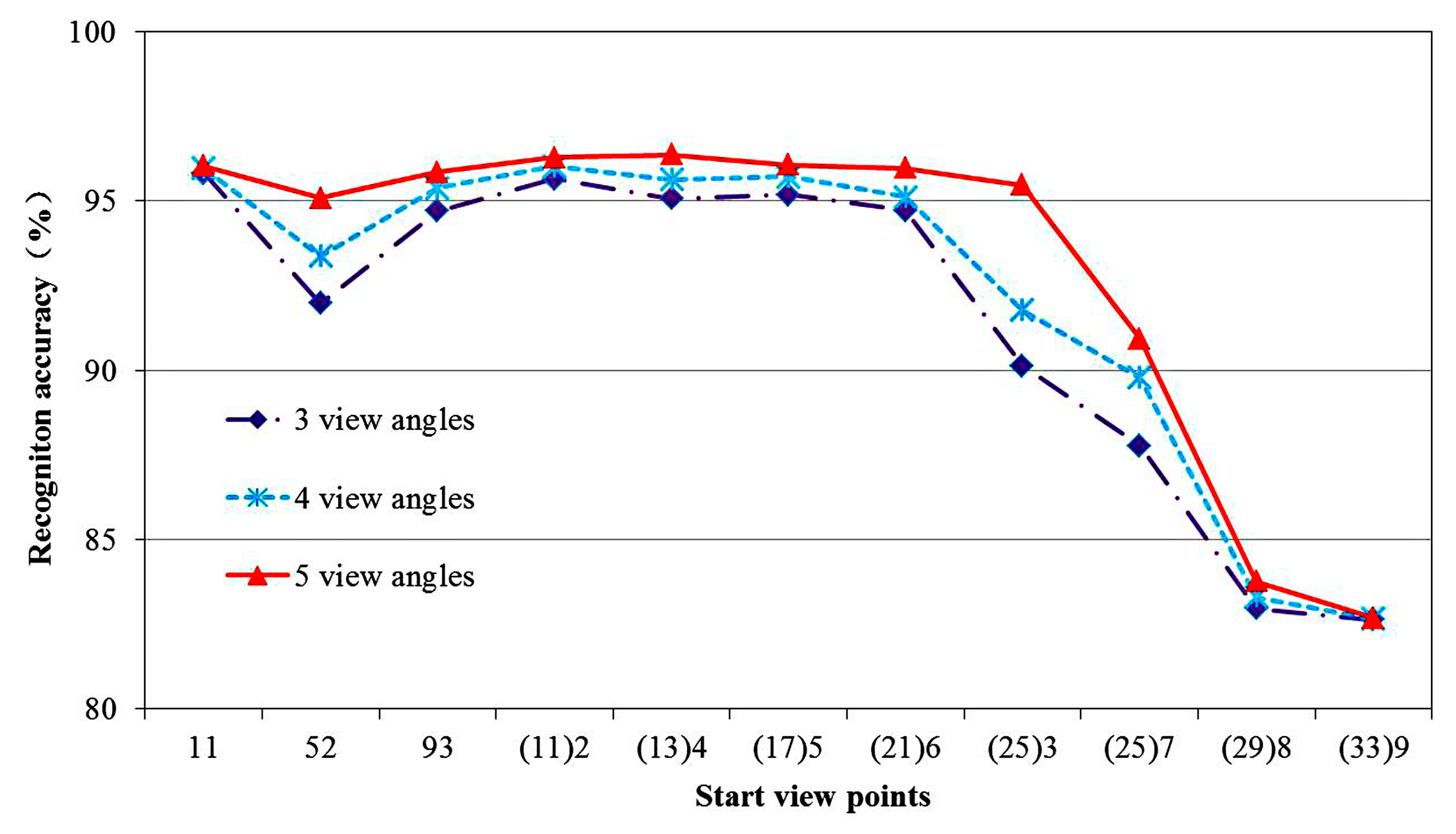
Representative starting points of different regions are selected to carry out the influence of different viewing angles on the recognition effect. As shown in Figure 15, the abscissa is the interval where the starting viewpoint is located, and the ordinate is the corresponding recognition rate. The dotted line with diamond mark represents the recognition rate with 3 viewing angles, the dotted line with * mark represents the recognition rate with 4 viewing angles, and the solid line with triangle mark represents the recognition rate with 5 view angles.

It can be seen from the Figure 15 that the recognition accuracy has a gradual downward trend, tending to the vertex of the hemisphere of the starting point. The starting point is at the 8th and 9th layers of longitude especially, because the set directed graph model is in a single direction. The more it tends to the vertex, the less the observation surface is, and the less the extracted features are. Even if the perspective is increased, the increase in recognition effect is not obvious due to the particularity of its location. Therefore, in practical application, try to avoid a starting point close to the top position. However, on the whole, the average recognition rate is 91.51% in the case of three viewing angles, 92.25% in the case of four viewing angles and 93.13% in the case of five viewing angles. The results show that the more viewing angles, the higher the target recognition rate. This method can obtain a higher recognition rate in an obstacle-free environment.

Through the above experimental analysis, it can be concluded that the proposed directed graph perspective optimization path planning method based on the A* algorithm considering the performance and efficiency of target recognition is feasible, and can obtain more accurate recognition results in a shorter path.

5. Conclusions

In order to enhance the robustness of vision-based robots in natural environment, a dynamic recognition method was used to improve the recognition performance. For the common linkage robots in industry, the end-camera was driven by a manipulator to complete the target observation with high accuracy efficiently in this paper. The perspective optimization path planning of the manipulator was studied, and the path planning method for finding optimal view angles based on the A* algorithm was proposed. An observation geometry model was established and the viewing angle intervals were divided. Based on the active viewpoint selection mechanism, a multi-view classifier based on BM2DKPCANet and Softmax was constructed. The output class probability was set as the viewpoint measure. The best identification performance and the shortest distances were taken as the objective functions of path planning. The directed graph programming model was constructed, and the directed graph adjacency matrix based on the planning distance was determined. The multi-objective optimization problem was transformed into the single-objective optimization problem by fusing the two adjacent matrices. The shortest path was planned based on the A* algorithm. The experiments were performed with different view count and different starting viewpoints. The results demonstrated that the method could plan the optimal path with higher recognition accuracy and efficiency.

References

- Vieira, T.; Bordignon, A.; Peixoto, A. Learning good views through intelligent galleries. Comput. Graph. Forum 2009, 28, 717–726. [Google Scholar] [CrossRef]
- Vázquez, P.P. Depth-based Automatic view selection through view stability analysis. Vis. Comput. 2009, 25, 441–449. [Google Scholar] [CrossRef] [Green Version]
- Leifman, G.; Shtrom, E.; Tal, A. Surface regions of interest for viewpoint selection. IEEE Trans. Pattern Anal. Mach. Intell. 2016, 38, 2544–2556. [Google Scholar] [CrossRef] [Green Version]
- Wang, W.; Yang, L.; Wang, D. Finding canonical views by measuring features on the viewing plane. In Proceedings of the Asia-Pacific Signal & Information Processing Association Annual Summit and Conference (APSIPA ASC), Hollywood, CA, USA, 3–6 December 2012; pp. 1–7. [Google Scholar]
- Feixas, M.; Sbert, M.; Gonzalez, F. A unified information-theoretic framework for viewpoint selection and mesh saliency. ACM Trans. Appl. Percept. 2009, 6, 1–23. [Google Scholar] [CrossRef]
- Sbert, M.; Plemenos, D.; Feixas, M.; Gonzalez, F. Viewpoint quality: Measures and applications. In Proceedings of the First Eurographics Conference on Computational Aesthetics in Graphics, Visualization and Imaging, Girona, Spain, 18–20 May 2005; pp. 185–192. [Google Scholar]
- Serin, E.; Sumengen, S.; Balcisoy, S. Representational image generation for 3D objects. Vis. Comput. 2013, 29, 675–684. [Google Scholar] [CrossRef]
- Gao, T.H.; Wang, W.C.; Han, H.L. Efficient view selection by measuring proxy information. Comput. Animat. Virtual Worlds 2016, 27, 351–357. [Google Scholar] [CrossRef]
- Shilane, P.; Funkhouser, T. Distinctive regions of 3D surfaces. ACM Trans. Graph. 2007, 26, 7. [Google Scholar] [CrossRef]
- Fu, H.B.; Cohen-Or, D.; Dror, G. Upright orientation of man-made objects. ACM Trans. Graph. 2008, 27, 42. [Google Scholar] [CrossRef] [Green Version]
- Mortara, M.; Spagnuolo, M. Semantics-driven best view of 3D shapes. Comput. Graph. 2009, 33, 280–290. [Google Scholar] [CrossRef]
- Chen, X.B.; Saparov, A.; Pang, B. Schelling points on 3D surface meshes. ACM Trans. Graph. 2012, 31, 29. [Google Scholar] [CrossRef]
- Hochreiter, S.; Schmidhuber, J. Long short-term memory. Neural Comput. 1997, 9, 1735–1780. [Google Scholar] [CrossRef] [PubMed]
- Li, J.; Chen, B.M.; Lee, G.H. So-net: Self-organizing network for point cloud analysis. In Proceedings of the IEEE Conference on Computer Vision and Pattern Recognition, Salt Lake City, UT, USA, 18–23 June 2018; pp. 9397–9406. [Google Scholar]
- Liu, A.A.; Zhou, H.; Nie, W.; Liu, Z.; Liu, W.; Xie, H.; Mao, Z.; Li, X.; Song, D. Hierarchical multi-view context modelling for 3d object classification and retrieval. Inf. Sci. 2021, 547, 984–995. [Google Scholar] [CrossRef]
- Wei, X.; Yu, R.; Sun, J. View-GCN: View-based Graph Convolutional Network for 3D Shape Analysis. In Proceedings of the 2020 IEEE/CVF Conference on Computer Vision and Pattern Recognition (CVPR), Seattle, WA, USA, 13–19 June 2020; pp. 1847–1856. [Google Scholar]
- Zhou, H.Y.; Liu, A.A.; Nie, W.Z.; Nie, J. Multi-View Saliency Guided Deep Neural Network for 3D Object Retrieval and Classification. IEEE Trans. Multimed. 2020, 22, 1496–1506. [Google Scholar] [CrossRef]
- Meng, F.; Xu, Y.; Huang, Z.; Wang, L. Optimal view selection method based on object detection. J. Phys. Conf. Ser. 2020, 1650, 032141. [Google Scholar] [CrossRef]
- Kanezaki, A.; Matsushita, Y.; Nishida, Y. Rotationnet: Joint object categorization and pose estimation using multiviews from unsupervised viewpoints. In Proceedings of the IEEE Conference on Computer Vision and Pattern Recognition, Salt Lake City, UT, USA, 18–23 June 2018; pp. 5010–5019. [Google Scholar]
- Kanezaki, A.; Matsushita, Y.; Nishida, Y. Rotationnet for joint object categorization and unsupervised pose estimation from multi-view images. IEEE Trans. Pattern Anal. Mach. Intell. 2019, 43, 269–283. [Google Scholar] [CrossRef] [Green Version]
- Chen, S.; Zheng, L.; Zhang, Y.; Sun, Z.; Xu, K. VERAM: View-Enhanced Recurrent Attention Model for 3D Shape Classification. IEEE Trans. Vis. Comput. Graph. 2019, 25, 3244–3257. [Google Scholar] [CrossRef] [Green Version]
- Sokolov, D.; Plemenos, D.; Tamine, K. Methods and data structures for virtual world exploration. Vis. Comput. 2006, 22, 506–516. [Google Scholar] [CrossRef]
- Alam, M.S.; Goodwin, S.D. Control of Constraint Weights for a 2D Autonomous Camera. In Canadian AI 2009: Advances in Artificial Intelligence, Proceedings of the Canadian Conference on Artificial Intelligence, Kelowna, BC, Canada, 25–27 May 2009; Springer: Berlin/Heidelberg, Germany, 2009; pp. 121–132. [Google Scholar] [CrossRef]
- Yao, Y.; Chen, C.H.; Koschan, A.; Abidi, M. Adaptive online camera coordination for multi-camera multi-target surveillance. Comput. Vis. Image Underst. 2010, 114, 463–474. [Google Scholar] [CrossRef]
- Amriki, K.A.; Atrey, P.K. Bus surveillance: How many and where cameras should be placed. Multimed. Tools Appl. 2014, 71, 1051–1085. [Google Scholar] [CrossRef]
- Guzman-Rivera, A.; Kohli, P.; Glocker, B.; Shotton, J.; Sharp, T.; Fitzgibbon, A.; Izadi, S. Multi-output learning for camera relocalization. In Proceedings of the 2014 IEEE Conference on Computer Vision and Pattern Recognition, Columbus, OH, USA, 23–28 June 2014; pp. 1114–1121. [Google Scholar] [CrossRef]
- Valentin, J.; Nießner, M.; Shotton, J.; Fitzgibbon, A.; Izadi, S.; Torr, P. Exploiting uncertainty in regression forests for accurate camera relocalization. In Proceedings of the IEEE Conference on Computer Vision and Pattern Recognition (CVPR), Boston, MA, USA, 7–12 June 2015; pp. 4400–4408. [Google Scholar] [CrossRef]
- Lan, K.; Sekiyama, K. Optimal Viewpoint Selection Based on Aesthetic Composition Evaluation Using Kullback-Leibler Divergence. In Proceedings of the International Conference on Intelligent Robotics and Applications ICIRA 2016: Intelligent Robotics and Applications, Tokyo, Japan, 22–24 August 2016; pp. 433–443. [Google Scholar]
- Qiu, Y.; Satoh, Y.; Suzuki, R.; Iwata, K.; Kataoka, H. Multi-View Visual Question Answering with Active Viewpoint Selection. Sensors 2020, 20, 2281. [Google Scholar] [CrossRef] [Green Version]
- Yokomatsu, T.; Sekiyama, K. Optimal viewpoint selection for indoor drones using PSO and Gaussian Processes. In Proceedings of the 2021 60th Annual Conference of the Society of Instrument and Control Engineers of Japan (SICE), Tokyo, Japan, 8–10 September 2021; pp. 634–639. [Google Scholar]
- Zou, Y.; Li, L.; Gao, Z. Obstacle avoidance path planning for harvesting robot arm based on improved PRM. Transducer Microsyst. Technol. 2019, 38, 52–56. [Google Scholar]
- Yuan, C.; Liu, G.; Zhang, W. An efficient RRT cache method in dynamic environments for path planning. Robot. Auton. Syst. 2020, 131, 103595. [Google Scholar] [CrossRef]
- Dai, W.; Li, C.; Yang, C.; Ma, X. Manipulator path planning using fusion algorithm of low difference sequence and rapidly exploring random tree. Control Theory Appl. 2022, 39, 130–144. [Google Scholar]
- Zhao, M.; Lv, X. Improved Manipulator Obstacle Avoidance Path Planning Based on Potential Field Method. J. Robot. 2020, 2020, 1701943. [Google Scholar] [CrossRef]
- Xu, T.; Zhou, H.; Tan, S.; Li, Z.; Ju, X.; Peng, Y. Mechanical arm obstacle avoidance path planning based on improved artificial potential field method. Ind. Robot 2022, 49, 271–279. [Google Scholar] [CrossRef]
- Fink, W.; Baker, V.R.; Brooks, A.J.-W.; Flammia, M.; Dohm, J.M.; Tarbell, M.A. Globally optimal rover traverse planning in 3D using Dijkstra’s algorithm for multi-objective deployment scenarios. Planet. Space Sci. 2019, 179, 104707. [Google Scholar] [CrossRef]
- Jia, Q.; Chen, G.; Sun, H.; Zheng, S. Path Planning for Space Manipulator to Avoid Obstacle Based on A* Algorithm. J. Mech. Eng. 2010, 46, 109–115. [Google Scholar] [CrossRef]
- Qureshi, A.H.; Simeonov, A.; Bency, M.J.; Yip, M.C. Motion planning networks. In Proceedings of the 2019 International Conference on Robotics and Automation (ICRA), Montreal, QC, Canada, 20–24 May 2019; pp. 2118–2124. [Google Scholar]
- Li, Y.; Liu, K. Two-degree-of-freedom manipulator path planning based on zeroing neural network. In Proceedings of the 2019 International Conference on Computer Science Communication and Network Security (CSCNS), Sanya, China, 22–23 December 2019; Volume 309. [Google Scholar]
- Zhang, J.; Cheng, L.; Wang, T.; Xia, W.; Yan, D.; Wu, Z.; Duan, X. A welding manipulator path planning method combining reinforcement learning and intelligent optimisation algorithm. Int. J. Model. Identif. Control 2019, 33, 261–270. [Google Scholar] [CrossRef]
- Hua, X.; Wang, G.; Xu, J. Reinforcement learning-based collision-free path planner for redundant robot in narrow duct. J. Intell. Manuf. 2020, 32, 471–482. [Google Scholar] [CrossRef]
- Zou, Q.; Liu, S.; Zhang, Y.; Hou, Y. Rapidly-exploring random tree algorithm for path re-planning based on reinforcement learning under the peculiar environment. Control Theory Appl. 2020, 37, 1737–1748. [Google Scholar]
- Wang, J.; Hirota, K.; Wu, X.; Dai, Y.; Jia, Z. Hybrid bidirectional rapidly exploring random tree path planning algorithm with reinforcement learning. J. Adv. Comput. Intell. Intell. Inform. 2021, 25, 121–129. [Google Scholar] [CrossRef]
- Santos, R.R.; Rade, D.A.; da Fonseca, I.M. A machine learning strategy for optimal path planning of space robotic manipulator in on-orbit servicing. Acta Astronaut. 2022, 191, 41–54. [Google Scholar] [CrossRef]
- Fang, Z.; Liang, X. Intelligent obstacle avoidance path planning method for picking manipulator combined with artificial potential field method. Ind. Robot 2021. ahead-of-print. [Google Scholar] [CrossRef]
- Su, H.; Maji, S.; Kalogerakis, E.; Learned-Miller, E. Multi-view convolutional neural networks for 3d shape recognition. In Proceedings of the IEEE International Conference on Computer Vision, Santiago, Chile, 7–13 December 2015; pp. 945–953. [Google Scholar]
- Gao, Z.; Wang, D.Y.; Xue, Y.B.; Xu, G.P.; Zhang, H.; Wang, Y.L. 3D object recognition based on pairwise Multi-view Convolutional Neural Networks. J. Vis. Commun. Image R. 2018, 56, 305–315. [Google Scholar] [CrossRef]
- Gao, Z.; Xue, H.; Wan, S. Multiple Discrimination and Pairwise CNN for view-based 3D object retrieval. Neural Netw. 2020, 125, 290–302. [Google Scholar] [CrossRef] [Green Version]
- Lin, C.H.; Kumar, A. Contactless and partial 3D fingerprint recognition using multi-view deep representation. Pattern Recognit. 2018, 83, 314–327. [Google Scholar] [CrossRef]
- Han, Z.; Shang, M.; Liu, Z.; Vong, C.; Liu, Y.; Zwicker, M.; Han, J.; Chen, C.L.P. SeqViews2SeqLabels: Learning 3D global features via aggregating sequential views by RNN with attention. IEEE Trans. Image Process. 2019, 28, 658–672. [Google Scholar] [CrossRef]
- Xu, H.; Wang, L.; Wu, Q.; Kang, W. PVLNet: Parameterized-View-Learning neural network for 3D shape recognition. Comput. Graph. 2021, 98, 71–81. [Google Scholar] [CrossRef]
- Zhang, Y.K.; Guo, X.S.; Ren, H.H. Multi-view classification with semi-supervised learning for SAR target recognition. Signal Processing 2021, 183, 108030. [Google Scholar] [CrossRef]
- Zhang, J.; Zhou, D.; Zhao, Y.; Nie, W.; Su, Y. MV-LFN: Multi-view based local information fusion network for 3D shape recognition. Vis. Inform. 2021, 5, 114–119. [Google Scholar] [CrossRef]
- Fei, L.K.; Zhang, B.; Wen, J. Jointly learning compact multi-view hash codes for few-shot FKP recognition. Pattern Recognit. 2021, 115, 107894. [Google Scholar] [CrossRef]
- Liang, Q.; Li, Q.; Zhang, L.; Mi, H.; Nie, W.; Li, X. MHFP: Multi-view based hierarchical fusion pooling method for 3D shape recognition. Pattern Recognit. Lett. 2021, 150, 214–220. [Google Scholar] [CrossRef]
- Li, X.N.; Wu, H.; Yang, X.H. Multi-view Recognition of Fruit Packing Boxes Based on Features Clustering Angle. High Technol. Lett. 2021, 27, 200–209. [Google Scholar]
- Li, X.N.; Wu, H.; Yang, X.H.; Xue, P.; Tan, S. Multi-view Machine Vision Research of Fruits Boxes Handling Robot Based on the Improved 2D Kernel Principal Component Analysis Network. J. Robot. 2021, 2021, 3594422. [Google Scholar]
- Chan, T.H.; Jia, K.; Gao, S. PCANet: A simple deep learning baseline for image classification. IEEE Trans. Image Process. 2015, 24, 5017–5032. [Google Scholar] [CrossRef] [Green Version]
Figure 1.
BM2DKPCANet model.
Figure 2.
Geometric model of hemispherical ring observation.
Figure 3.
Multi-view classifier.
Figure 4.
Two-view classifier.
Figure 5.
Recognition performance digraph.
Figure 6.
Path planning flow chart based on A* algorithm.
Figure 7.
Experimental platform.
Figure 8.
Partial calibration figures.
Figure 9.
Structure of MoveIt! package.
Figure 10.
Viewpoint optimization path planning.
Figure 11.
End three-dimensional path map.
Figure 12.
Three-view optimal observation paths.
Figure 13.
Four-view optimal observation paths.
Figure 14.
Five-view optimal observation paths.
Figure 15.
Recognition performance with different start points and view angles.