Finding All Solutions and Instances of Numberlink and Slitherlink by ZDDs
by
Ryo Yoshinaka
1, 
Toshiki Saitoh
2,3,*,
Jun Kawahara
2,3,
Koji Tsuruma
2,
Hiroaki Iwashita
2,3 and
Shin-ichi Minato
2,3 1
Graduate School of Informatics, Kyoto University, Kyoto, 606-8501, Japan
2
ERATO MINATO Project, Japan Science and Technology Agency, Kitaku North 14, West 9, Sapporo, 060-0814, Hokkaido, Japan
3
Graduate School of Information Science and Technology, Hokkaido University, Kitaku North 14, West 9, Sapporo, 060-0814, Hokkaido, Japan
*
Author to whom correspondence should be addressed.
Algorithms 2012, 5(2), 176-213; https://0-doi-org.brum.beds.ac.uk/10.3390/a5020176
Submission received: 16 November 2011
/
Revised: 29 February 2012
/
Accepted: 19 March 2012
/
Published: 5 April 2012
(This article belongs to the Special Issue Puzzle/Game Algorithms)
Abstract
:Link puzzles involve finding paths or a cycle in a grid that satisfy given local and global properties. This paper proposes algorithms that enumerate solutions and instances of two link puzzles, Slitherlink and Numberlink, by zero-suppressed binary decision diagrams (ZDDs). A ZDD is a compact data structure for a family of sets provided with a rich family of set operations, by which, for example, one can easily extract a subfamily satisfying a desired property. Thanks to the nature of ZDDs, our algorithms offer a tool to assist users to design instances of those link puzzles.
1. Introduction
Link puzzles, for example Slitherlink, Numberlink, Masyu, etc., are logic puzzles that involve finding paths or a cycle in a grid that satisfy given local and global properties. This paper focuses on two simple link puzzles, Numberlink and Slitherlink, amongst others.
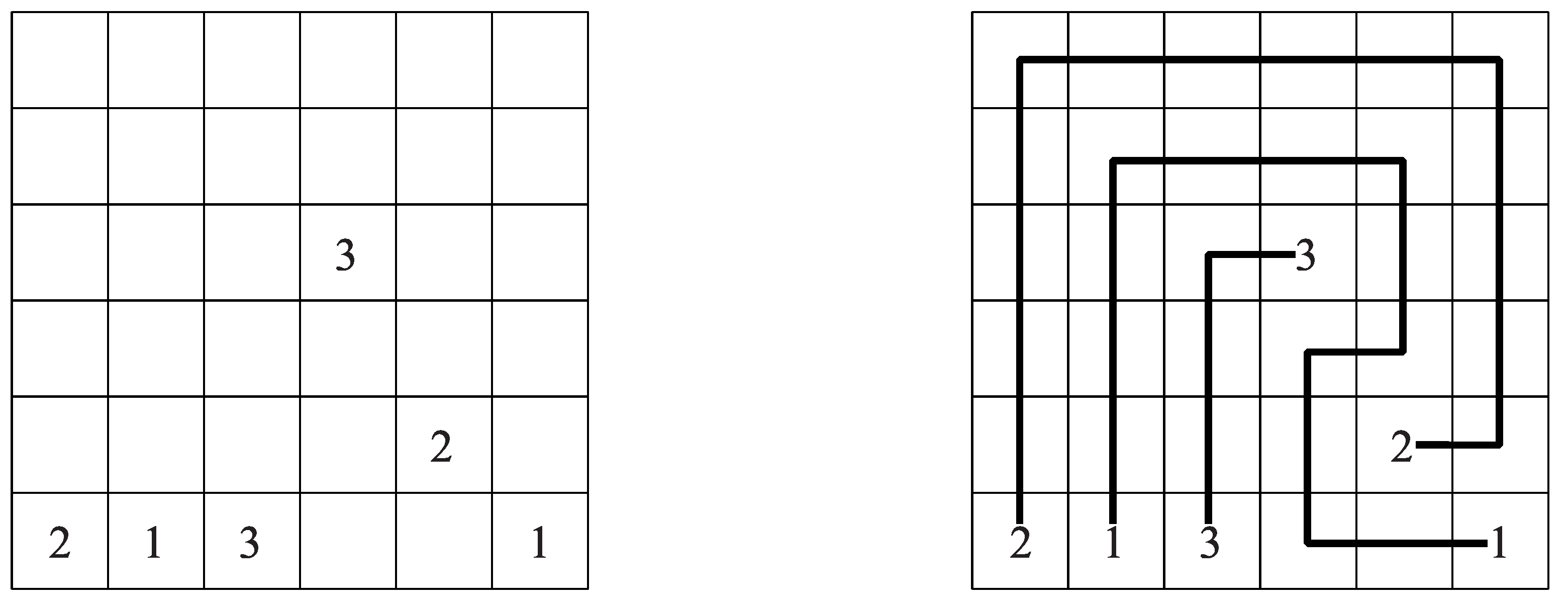
Numberlink is played on a grid where the rules are below [1].
- Connect pairs of the same numbers with a continuous line.
- Lines go through the center of the cells, horizontally, vertically, or changing direction, and never twice through the same cell.
- Lines cannot cross, branch off, or go through the cells with numbers.
Figure 1 describes an instance of Numberlink. Numberlink is known to be NP-complete [2,3,4]. Numberlink is also studied as a model of VLSI layout design [5].
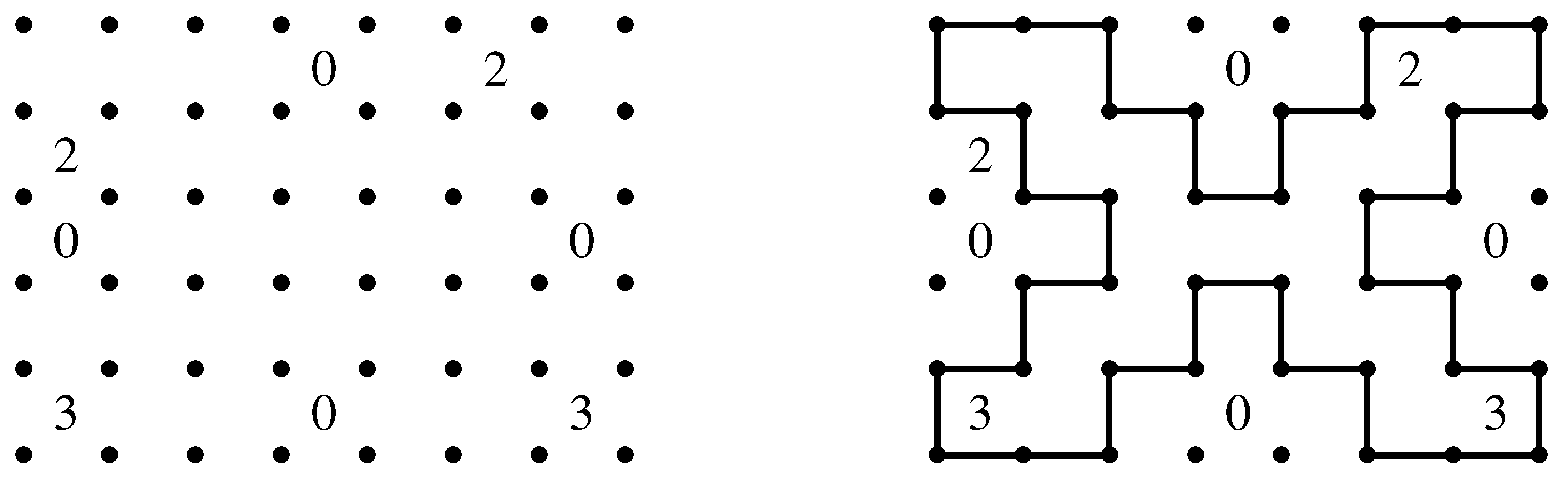
Slitherlink is played on a grid of lattice dots where we draw a loop satisfying below [1].
- Connect adjacent dots with vertical or horizontal lines.
- A single loop is formed with no crossing or branches.
- The numbers indicate how many lines surround it, while empty cells may be surrounded by any number of lines.
Link puzzles have been popularized by a Japanese publisher Nikoli and many puzzle designers are trying to produce good and interesting instances. The least common criterion on instances to be good is to admit exactly one solution, but what should be good and interesting is quite a subjective issue to respective designers. The complexity barrier suggests difficulties in the instance design.
On the other hand, as is usually the case for logic puzzles, computer scientists and programmers have been proposed several automatic solvers targeting those link puzzles. Sugar [8] is a SAT based constraint solver which is provided with formulation of Numberlink and Slitherlink. While it is often the case that a solution for an instance of Numberlink is found just by inspiration, many local solution methods for Slitherlink are known. Most Slitherlink solvers employ such methods [9,10,11].
Moreover, there are some attempts to automatically generate instances of Slitherlink. Shirai’s algorithm [10] starts from a grid graph with no numbers, which admits many solutions, and repeatedly puts a random number into a random cell one by one until the obtained instance admits a unique solution. The opposite approached has been proposed by Shirai et al. [10] and Wan [11]. Their algorithm takes a cycle, which is a predetermined solution, as input and starts from a grid whose cells are all fulfilled by the numbers compatible with the solution. The algorithm then repeatedly removes the number in a random cell one by one until the obtained instance admits an unexpected solution. The algorithm outputs the instance obtained just before removing the last number.
Our contribution is located in this line of research. We propose solution and instance enumeration algorithms for Numberlink and Slitherlink. Unlike existing algorithms, ours output all the qualified solutions/instances at once in the form of a zero-suppressed binary decision diagram (ZDD). A ZDD is a compressed data structure for representing and manipulating families of sets [12]. Recently, Knuth [13, exercise 225] has proposed an algorithm, called Simpath, that constructs a ZDD representing all s-t paths on a given graph and two vertices s and t, where a path is identified with the set of edges constituting the path. If an instance of Numberlink has only one pair of numbers in a grid, Simpath gives all solutions to it. Knuth has also proposed a modification of Simpath that enumerates all single cycles on an input graph in the form of a ZDD. Recall that to be a cycle is a necessary condition to be a solution for Slitherlink. Our solvers for the link puzzles construct a ZDD representing solutions in the manner of Simpath with taking the constraints from the problem instance into account. By the nature of enumeration, one can immediately decide whether an instance admits exactly one solution.
ZDDs can represent families of sets in a small space, yet an even more important and widely appreciated virtue of ZDDs is that one can quite efficiently perform fundamental mathematical operations on families of sets over ZDDs, like union, intersection, etc. Our algorithms for generating instances of the link puzzles apply the virtue of ZDDs. Our method based on ZDDs offers users flexible means to design puzzle instances. For example, puzzle designers can extract some specific kind of instances from the whole which they think “interesting” by those set operations over ZDDs.
This paper is organized as follows. Formal definitions of ZDDs, Numberlink and Slitherlink are given in Section 2. Section 3 introduces a variant of Simpath that enumerates all path matchings over a graph, on which other algorithms of ours are based. Our Numberlink solver is presented in Section 4 and Numberlink instance enumeration algorithm is proposed in Section 5. On the other hand, our Slitherlink solver and instance enumeration algorithm are presented in Section 6 and Section 7, respectively. We also show experimental results on these algorithms in Section 8, where we compare the performance of known solving algorithms and ours. Moreover, we demonstrate how our method may help puzzle designers through presenting visually attractive instances of Slitherlink obtained by our algorithm. We then conclude the paper in Section 9.
2. Preliminaries
2.1. Zero-Suppressed Binary Decision Diagrams
A zero-suppressed binary decision diagram, ZDD for short, represents a family of sets over a universal set E whose elements are linearly ordered [12]. We index the elements of E as where we write if and only if . A ZDD is defined to be a labeled directed acyclic graph that satisfies the following properties.
- There is only one node with indegree 0, called the root node.
- There are just two nodes and with outdegree 0, called the 0-terminal and 1-terminal.
- Each node except terminals has just 2 outgoing arcs, which are labeled by 0 and 1 and called the 0-arc and 1-arc, respectively. We call the node pointed by the j-arc of a node n the j-child of n.
- Each node n except for the terminals is labeled by an element of E.
- The label of a non-terminal node is strictly smaller than those of its children.
If a node n is the j-child of another node , we call a j-parent of n for . We say that a path from the root node of a ZDD Z is valid if it ends in a node which is not . To each valid path we assign a set by
By representing a path from the root node of a ZDD by a sequence of 0 and 1, which we call a -sequence, we have an alternative inductive definition of the set:
where e is the label of the node in which ends. Each node is assigned a set defined by
An equivalent inductive definition is given by
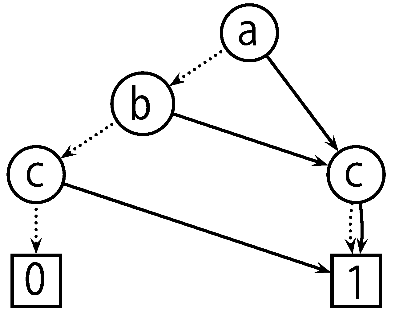
The family of sets that a ZDD represents is defined to be . Figure 3 shows an example of a ZDD.
A ZDD is said to be reduced if
- there is no distinct nodes that have the same label, 0-child and 1-child,
- there is no node whose 1-child is .
It is known that every ZDD admits a unique reduced one that represents the same family of sets. Moreover the number of nodes of a ZDD is minimum amongst ZDDs representing the same family if and only if it is reduced. A linear-time algorithm that reduces a ZDD can be found in [13, pp. 84–85, algorithm R].
A (reduced) ZDD can represent a family of sets in a compact way by letting multiple sets in the family share some subgraphs of the ZDD. If sets in the family have some “regular” structures, the size of the ZDD can be logarithmically smaller than the sum of the cardinalities of the sets in it. An even more important and widely appreciated virtue of ZDDs is that one can efficiently perform fundamental mathematical operations on families of sets over ZDDs, like union, intersection, etc. The efficiency depends on the size of the ZDDs rather than the cardinality of the sets in the target families. Some packages of implementation of ZDDs are provided to users of different purposes, where for given two ZDDs representing families of sets A and B, it can compute the ZDD for , , , and so on. For , it can compute the ZDD for , , etc. Knuth [13] has discussed further operations for families of sets, which enable us to extract maximal elements , minimal elements among others. For more details of ZDDs, readers are referred to [12,13], for example.
2.2. Undirected Graphs
The link puzzles concerned in this paper are played on undirected graphs. This paper uses ZDDs to represent subgraphs of graphs of puzzle instances. To avoid confusion among objects of those two kinds of graphs simultaneously in concern, we reserve words “nodes” and “arcs” for ZDDs, while we call the corresponding notions for graphs of puzzle instances “vertices” and “edges”.
An undirected graph is a pair where V is a set of vertices and is a set of edges, which are sets of exactly two elements of V. An edge is said to be incident to if . The degree of a vertex v in G is defined by , that is, the number of edges incident to v. For an edge set , we also define the degree of v in by . A vertex v is isolated if its degree is 0.
A nonempty edge set is called a simple path (or just a path) if there are pairwise distinct vertices such that for . The path P is also called a - path.
A nonempty edge set is called a (simple) cycle if and there are pairwise distinct vertices such that and for .
A possibly empty edge set is called a path matching if there are simple paths with such that and for distinct (For a family P of sets over a universal set V, we define .). We remark that for a path matching P, a way of partitioning P into paths satisfying this definition is unique. We say that P contains a u-v path if one of such paths is a u-v path.
A family of sets over V is called a pair matching if T consists of pairwise disjoint sets of size 2.
Lemma 1.
For a graph , an edge set is not a path matching if and only if there is a vertex of degree more than 2 in P or there is a subset that is a simple cycle.
2.3. Link Puzzles
Definition 2
(Numberlink). An instance of the Numberlink problem is a pair of a graph (Usually the graph G in an instance is a rectangular grid as described in the introduction, but this paper targets the more general problem described here.) and a pair matching h on V. A path matching on G is said to be a solution of if and only if it contains paths for all but no other.
An instance of the Numberlink problem is said to be good if admits exactly one solution P and moreover the unique solution P covers every vertex: i.e., .
Definition 4
(Slitherlink). An instance of the Slitherlink problem is a pair of a graph and a partial mapping such that for all , where denotes the domain of h (Usually G is a grid graph and is defined only when is a cycle consisting of just four edges.). We call h a hint assignment. A solution of is a cycle C over G such that for all . An instance of the Slitherlink problem is said to be good if admits exactly one solution.
Theorem 5.
[14] For input G and h, deciding whether admits a solution is NP-complete. For input and a solution C, deciding whether admits another solution is NP-complete.
In this paper, we assume that G is connected on both puzzles.
3. ZDD for Path Matchings
Knuth has proposed an algorithm that constructs a ZDD representing all the s-t paths on a given graph G and two vertices s and t in G, as an answer to Exercise 225 in [13]. Based on Knuth’s algorithm, this section presents an algorithm that constructs in a topdown manner a ZDD representing all the path matchings over a graph . This algorithm prepares for our puzzle solvers.
Let be an undirected graph. The edge set is the universal set of , where we have if and only if . We define . The root node of is labeled with and if a node is labeled with then its children are labeled with unless they are terminal nodes, or . By we denote the set of nodes with the label for . Hence is the singleton of the root node and consists of the children of nodes in . Every valid path ending in has length in . For a -sequence , we denote the length of by . For with , we define
We then have if is a valid path in . For a valid path , we let denote the node in which ends. We have . The ZDD will be constructed so that
Note that every subgraph of a path matching is a path matching.
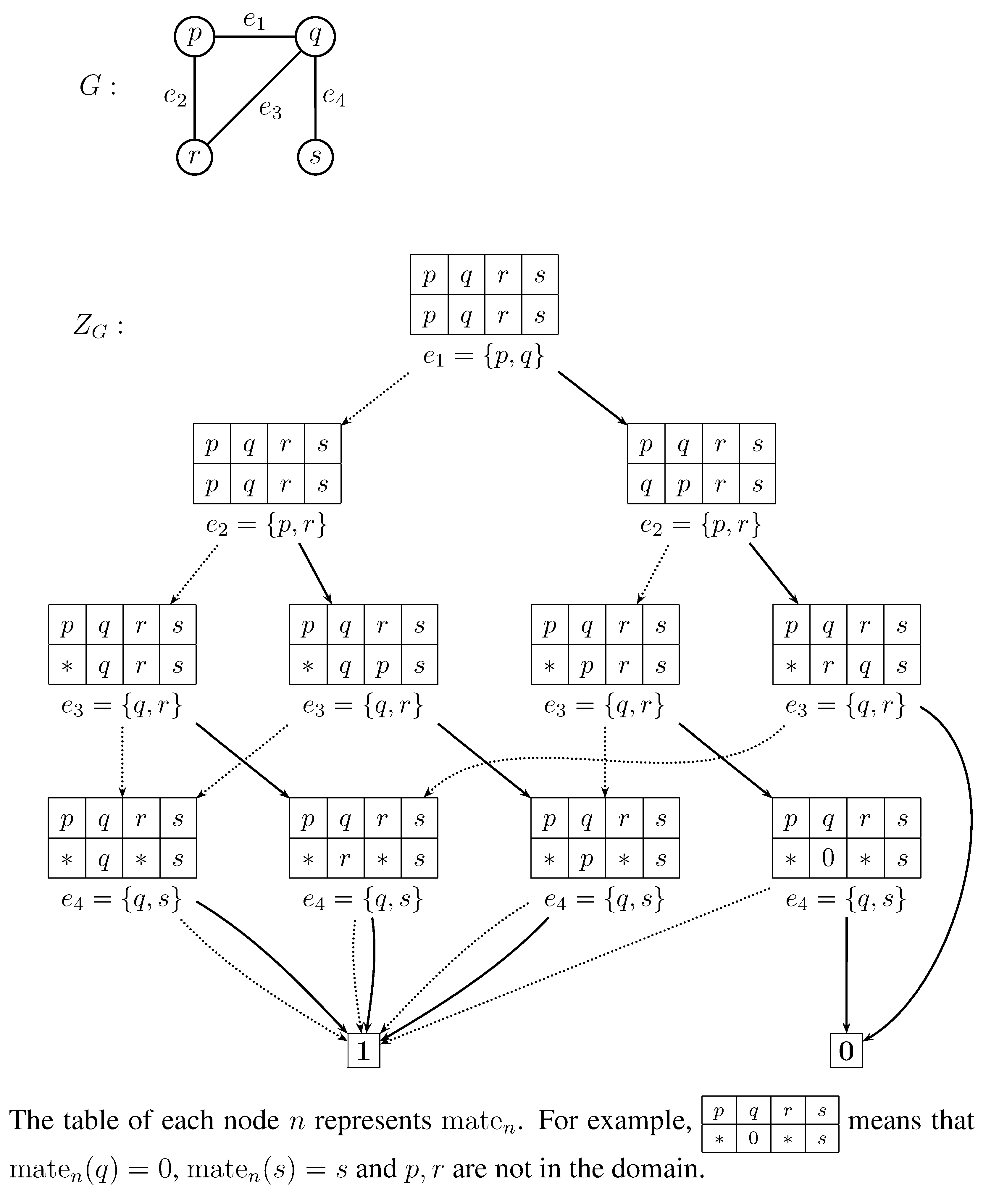
Our algorithm constructs in a top-down manner. The construction consists of phases, where we create nodes in as children of nodes in in the ith phase. Figure 4 illustrates an example of G and , which would help the reader understand our algorithm. We first initialize to be empty for all and to be the singleton of the root node . We create nodes in after the upper part of consisting of the nodes in and the arcs among them have been constructed for .
The algorithm stores some topological information of the path matching at the node reached by a valid path . Let , where we have and n is labeled by unless . We assign the node n a function , which we call a mate function, where and . It is determined so that
for each . In other words, if v has degree 0 in , and if v has degree 2 in . Particularly for the root node , we have for all ; the set is identical to V, since G has no isolated vertices. The domain of a mate function is restricted to , which is the set of vertices to which at least one edge in is incident. We are not interested in the topological information on vertices that we will not visit any more. Note that . Hereafter we stipulate that denotes the empty set.
In the example of Figure 4, we have , and . For , is a path matching consisting solely of a q-r path. The domain of the mate function is and , and .
Let us consider the ith phase of our algorithm, where we already have constructed an incomplete ZDD until the nodes in . We determine the children of a node for a valid path . The arcs given in this phase correspond to the choice whether or not we pick in a path matching. Let .
Giving a 0-child to n involves no difficulty. By assumption is a path matching and by definition . We create a node in as the 0-child of n and label by . That is, . The mate function of should be identical to except that the domain may be smaller than . In the case where , the 0-child of n is .
On the other hand, and it is not always the case that is a path matching. If is not a path matching, the 1-child of n should be . Otherwise, we give a node with an appropriate mate function as the 1-child of n. We must decide whether is still a path matching or not. Let . We note that u and v are in the domain of . There exist several cases depending on the topology of . Recall that an edge set is a path matching if and only if the degree of every node in P is at most 2 and no subset is a cycle. In the case where , the degree of u in is 2, so the degree of u will be 3 in , which is therefore not a path matching. The same holds when . Moreover, if (equivalently ), which means that contains a u-v path , then contains a simple cycle . We say that a mate function m rejects an edge if or . If rejects , then is not a path matching, hence the 1-child of n should be . On the other hand, if does not reject , is a path matching. So we need to give a node as the 1-child of n. Particularly in the case where , the 1-child of n will be . If , we create a node in as the 1-child of n (i.e., ) and assign a function that is consistent with the requirement of Equation (2). Actually one can compute from and by
for .
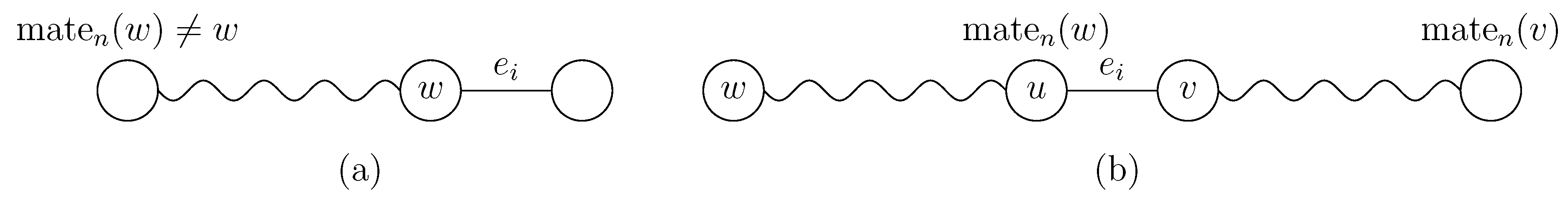
We explain why this is correct. The first case means that w has degree 1 in . Hence, the degree of will be 2 in (Figure 5(a)). In the second case, means either that has a w-u path or that and w is isolated in . It is convenient for explanation to regard an isolated vertex t as a t-t path. According to this terminology, contains a w-u path and a v- path. Then the edge will bridge those paths: contains a w- path (Figure 5(b)). The third case is similar to the second case. If none of those three cases apply, adding does not matter for the vertex w. We note that by the assumption, the first three cases are mutually exclusive.
Summarizing the above, by observing , one can determine whether is a path matching or not. Moreover one can compute both and for the 0-child and 1-child of n, respectively, unless they are or . Consequently, if two nodes and with the same label have the same mate function, their descendants will constitute subgraphs of exactly the same shape in . This means that such equivalent nodes and should be merged before generating children.
Our actual algorithm, shown as Algorithm 1, maintains each node set not to contain distinct nodes assigned the same mate function. This is realized by a procedure named (short for “getting a node”) which takes two arguments: an edge index and a mate function m. returns a node labeled and assigned m. If such a node has already been created in , that node is returned. Otherwise, we create one in and return it. It is conveniently assumed that gives the terminal node . Note that this procedure may update .
| Algorithm 1: Enumeration of path matchings |
 |
For a node labeled and assigned a mate function m which does not reject , the mate function of its 1-child is given by in Algorithm 1, which is determined in the way described in Equation (3). That is, (short for “mate update”) takes a mate function m and an edge and returns a mate function defined by
for each . The domain of is the same as that of m. By we denote the subfunction of whose domain is restricted to .
We prove the correctness of Algorithm 1 in Appendix A.
4. Numberlink Solver
This section presents a Numberlink solver, which constructs a ZDD that represents all the solutions for a given instance of Numberlink. Recall that a solution for an instance of Numberlink is a path matching that satisfies a property represented by the pair matching h. It is in fact rather easy to modify Algorithm 1 to obtain a Numberlink solver.
Let us consider when we should connect an arc of a node to in addition to the cases we have discussed in Section 3. Suppose that we have chosen edges from and by picking up other edges from , we would like to form a solution. Let be a -sequence of length i that represents the choice. It is easy to see that if one of the following conditions holds, cannot be a solution of for any edge set .
- is not a path matching,
- there is of degree 2 in ,
- there is of degree 0 in ,
- there are such that contains a u-v path and ,
- there is a vertex of degree 1 in .
Our Numberlink solver, shown as Algorithm 2, constructs a ZDD so that if a path of length i satisfies one of the above, then (a prefix of) leads to . While Algorithm 1 connects no 0-arcs to , our Numberlink solver sometimes connects 0-arcs to according to the above conditions. This judgement is realized by observing the mate functions. For a mate function and an edge index i, we say that is incompatible with h if for some, one of the following conditions holds.
- and ,
- and .
When is incompatible with h for , the 0-arc of n should be connected to , since cannot be a solution for any . In the first case, the degree of is 0 in P. In the second case, the degree of is 1 in P.
| Algorithm 2: Numberlink solver |
 |
We prove the correctness of Algorithm 2 in Appendix B.
We say that is incompatible with h if for , one of the following conditions holds.
- m rejects , i.e., ,
- and ,
- and .
When is incompatible with h for , the 1-arc of n should be connected to , since cannot be a solution for any . In the first case, P is not a path matching. In the second case, v has degree more than 1 in P. In the third case, either P contains a - path or the degree of or is more than 1 in P.
Remark 6.
It is obvious that no proper superset of a solution for can be another solution. One can modify Algorithm 2 so that a path directly leads to if is a solution. Replace by where
Remark 7.
An alternative definition of Numberlink requires a solution to cover all the vertices. This constraint drastically shrinks the search space. It is easy to modify our algorithm to obtain only such strict solutions. We say that is incompatible with h if it is incompatible in the above sense or there is such that , which means that v is not covered.
5. Numberlink Instance Enumeration
This section presents an algorithm that enumerates all pair matchings h that give a good instance of the Numberlink problem for a given graph G. Fixing G, we say that a pair matching h is good if is a good instance. Let us first consider an easier task, which enumerates all the instances that admit at least one solution. A solution for an instance of the Numberlink problem is a path matching and conversely every path matching P on G consisting of - simple paths for all is a solution for where consists of for all. Our instance enumeration algorithm, shown as Algorithm 3, is again based on Algorithm 1, but now what we should enumerate is not edge sets but rather pair matchings. The ZDD output by Algorithm 1 will be a part of the input of Algorithm 3.
For a valid path in , the corresponding path matching consists of two kinds of simple paths: fixed paths and unfixed paths. Fixed paths are u-v paths where . In other words, every fixed path in will be a constituent of any path matching represented as (We note that whether a simple path in a path matching is fixed or unfixed depends on rather than itself. Yet we prefer a concise phrasing relying on the reader’s flexibility and assume that the vertex set in concern is understood.). We note that by definition does not tell us whether contains a fixed u-v path. On the other hand, the presence of an unfixed u-v path is observed in the mate function. If a u-v path is unfixed, at least one of is in . Without loss of generality, we assume , where we have . Since u has an incident edge in , the path may be extended so that u has degree 2.
| Algorithm 3: Numberlink Generator |
 |
We prove the correctness of Algorithm 3 in Appendix C.
Let denote the pair matching corresponding to the ends of fixed paths:
Note that for any and as long as is a path matching. We decorate each node n of the ZDD with the family
When a path ends in in , all the simple paths constituting are fixed. By definition, will be the family of pair matchings h such that admits a solution. For different valid paths and ending in the same node , and may have different fixed paths, but they share the same unfixed paths. We present an example of and in Appendix F.
Let us think about how to compute the family of a node n from the pair matching families assigned to its parents . By definition, it is not hard to see that
where . Define
We now have
for both . Therefore, for ,
In this way, one can recursively compute for all nodes except of .
We would like to extract good ones from . In addition to , we assign each node n another family such that no pair matching will be expanded to a good one. We construct so that
This definition is explained as follows. For the first line Equation (4), suppose that there are distinct valid paths and ending in the same node such that . Then, is a path matching if and only if so is for any . Moreover, consists of - paths for for some k if and only if so does . That is, the instance has two distinct solutions and . The second part Equation (5) of the definition of is easier. If , then there is a vertex which has degree 0 in and thus in for any . If is a path matching consisting of - paths for for some k, the instance has a solution that does not cover all the vertices.
We can compute the family of a node n from the pair matching families assigned to its parents according to the definition of :
where for . The lines Equations (6) and (7) come from Equations (4) and (5), respectively. Suppose that . Then regardless of whether it is due to Equation (4) or Equation (5), we have for any as long as is valid. Those pair matchings are captured by Equation (8).
6. Slitherlink Solver
The goal of this section is to give a Slitherlink solver, which constructs a ZDD that represents all the solutions for a given instance of Slitherlink. Recall that a solution is a simple cycle that satisfies a property represented by the hint assignment . As a preparation, we present an algorithm that constructs a ZDD representing all the simple cycles on a given graph G. Actually this algorithm is an answer to Exercise 226 of [13].
Based on the fact that any proper subgraph of a cycle is actually a path matching, it is easy to modify Algorithm 1 so that simple cycles shall be enumerated. We allow vertices to have degree 1 temporarily during the construction, but when we have determined which of the edges incident to a vertex v shall be used, the degree of v must be 0 or 2. In addition, we allow to add an edge to a path matching if consists solely of a single u-v path: it completes a cycle.
Both conditions are judged by observing the mate functions. We say that a mate function m and an edge form a cycle if for any v in the domain of m,
If and form a cycle for , the 1-child of n should be .
We say that has a fixed end if
For a valid path in , if has a fixed end, has a vertex of degree 1 for any . We say that mdeclines if either m rejects or has a fixed end. If declines for , the 1-child of n should be .
In addition, since the empty edge set is not a cycle, the corresponding path in our ZDD should end in .
Algorithm 4 constructs a ZDD for representing all the simple cycles on a graph G. We prove the correctness of Algorithm 4 in Appendix D.
| Algorithm 4: Enumeration of simple cycles |
 |
We are now ready to give our Slitherlink solver, shown as Algorithm 5, based on Algorithm 4.
| Algorithm 5: Slitherlink solver |
 |
Let be a Slitherlink instance. To ensure that the computed cycle is compatible with the hint assignment h, we assign another function to each node n in addition to . The function counts the number of picked edges in D in the domain of h. That is, for a valid path , we shall have for each . Especially for each . Updating the counter is very easy. For a mapping and an edge , we define (it stands for “counter update”) by
for every .
For of length i, when it is clear that there is no such that is compatible with h, the path should end in . We say that is incompatible with h if there is such that either
- or
- .
We say that cmatches h if for all .
The function is modified so that it handles a counter function in addition to a mate function. It takes an edge index , a mate function m and a counter function c. returns a node labeled and assigned m and c. If such a node has already been created in , that node is returned. Otherwise, we create one in and return it. Note that this procedure may update .
We give a formal proof for the correctness of Algorithm 5 in Appendix E.
7. Slitherlink Instance Enumeration
In this section, we discuss instance enumeration for the Slitherlink problem, assuming that a graph , a solution cycle C over G, and the maximum domain of hint assignments are given. Let be a hint assignment such that for all . The objective is to enumerate every that leads to a good instance of the Slitherlink problem such that and for all . A good instance must not have any compatible cycles other than C. Therefore, the instance enumeration problem is solved by computing
where is the set of all cycles on G. We use Algorithm 4 to construct a ZDD for . For this sake, we invoke the dynamic virtue of ZDDs that allows us to perform mathematical set operations quite easily.
A ZDD for the family can be regarded as a function such that
where is a vector of binary variables representing if each edge is taken. A ZDD for can also be regarded as a function such that
Let be a vector of binary variables representing if the ith element of is included in . Now we can rewrite Equation (9) in terms of x and y as follows, which can be computed by conventional operations on ZDDs:
Once is computed, ZDD operations enable us to restrict it easily to some interesting subset, such as instances with the minimum or minimal hints, and to output all instances explicitly.
8. Experiments
The following experiments for the Numberlink solvers, the Slitherlink solvers and the Slitherlink generators are performed on AMD Opteron Processor 8393, 3.09 GHz with 512 GB memory running SuSE 10, and those for the Numberlink generators are performed on AMD Opteron Processor 6136, 2.40 GHz with 256 GB memory running SuSE 10.
8.1. Solvers for Numberlink and Slitherlink
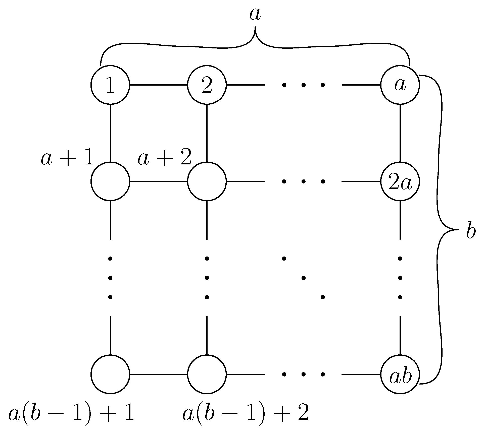
In this subsection, we discuss our experimental results on the comparison of our algorithm for solving Numberlink and Slitherlink with existing methods which are based on CPLEX 12.3 and Sugar. We implemented Algorithm 2 for Numberlink solver and Algorithm 5 for Slitherlink solver in C and compiled them by G 4.6 with -O3 optimization option. In our implementation, a variable order (an edge order) is lexicographical on sets of two vertices where vertices are labeled such as Figure 6.
We prepared the benchmark programs. We formulated solving Numberlink [15] and Slitherlink [16] as integer programs and solve them by CPLEX, which is an integer programming solver. Sugar is a SAT based constraint solver [8]. Sugar provides the formulation of Numberlink [17] and Slitherlink [18]. We also compared them with a heuristic solver slink [9] specialized for Slitherlink, which is published as a C source code.
Table 1 shows the running times of these methods for solving Numberlink. In the table, BNx denotes the xth instance in [19]. C88 is the Vol. 88 instance in Puzzle Championships 2010 [20]. Let denote the grid graph. In Table 2, we show the running times of these methods with the restriction that requires solutions to cover all vertices (see Remark 7).
Table 3 describes the running time of these methods as Slitherlink solvers. BSx denotes the xth instance in [21]. S10 is a large sample problem on [22]. C95 is the Vol. 95 instance in Puzzle Championships 2010 [20].
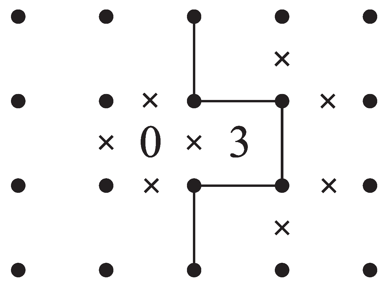
This table shows that slink is by far the fastest. A reason is that slink is a heuristic solver for Slitherlink which uses information specialized for Slitherlink. For example, when two adjacent cells are assigned “0” and “3” respectively, 12 of the surrounding edges are immediately determined to be or not to be in any solution (see Figure 7).
8.2. Numberlink Generator
In this subsection, we show experimental results for enumerating all Numberlink instances for grid graphs by a variant of Algorithm 3. Our actual implementation is purely top-down, which is different from Algorithm 3. By interweaving the idea of Algorithm 3 into Algorithm 1, we construct assigning nodes mate functions as well as pair matching families representing the ends of fixed paths simultaneously. In our algorithm, and are calculated by set operations such as union and intersection. We implemented these sets by ZDDs whose variables are unordered pairs of vertices . For efficiency, our implementation maintains instead of for each node n in , where .
Table 4, Table 5 and Table 6 show the running time of our algorithm, the number of good instances and that of nodes of for .
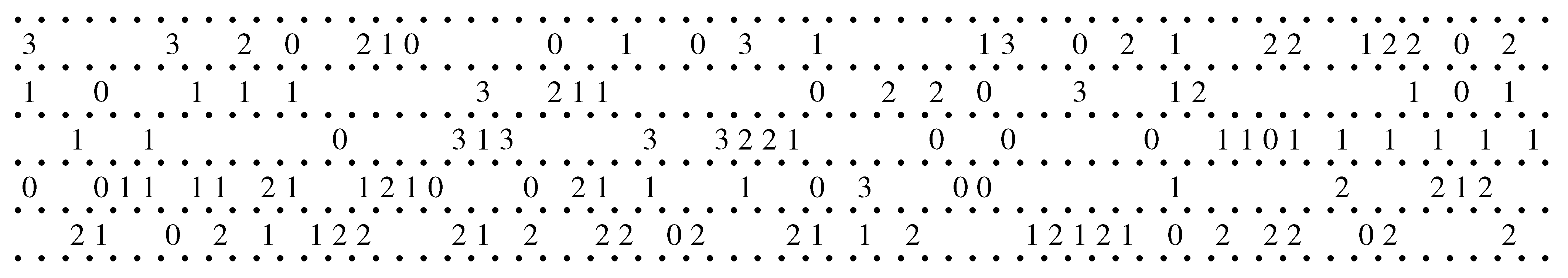
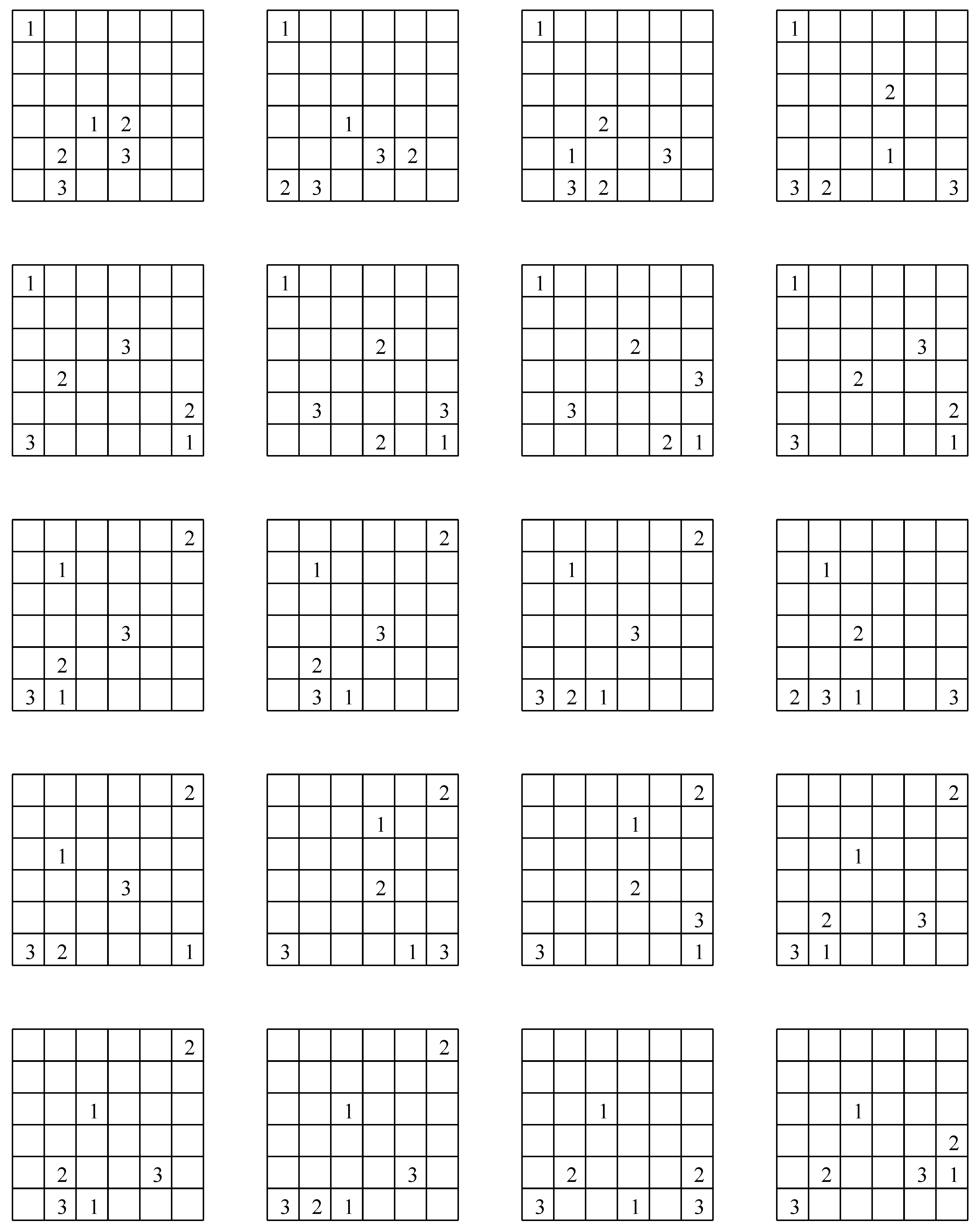
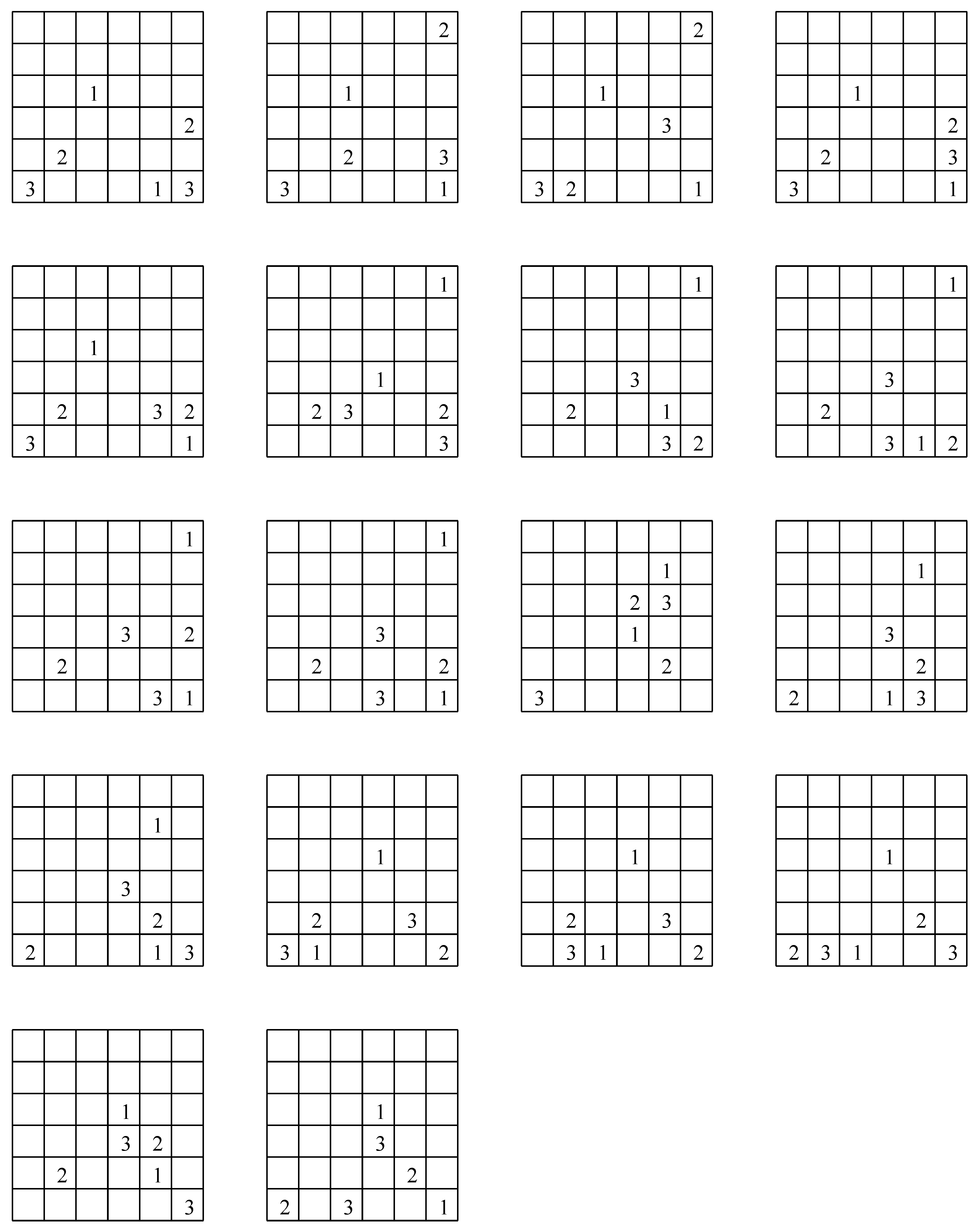
For , the computation did not finish within one week. We tried to compute the number of instances with restricting the number of pairs to at most ℓ. Table 7 shows the result of this computation for and . Let and . We maintain instead of in each node n. We omit the method of computing and . Then, we obtain that the number of minimum pairs with which gives a good instance is 3 from this result. We give the complete list of those instances on the graph with 3 pairs of vertices in Appendix G.
8.3. Slitherlink Generator
For the Slitherlink generator, we tried to generate some interesting examples of Slitherlink instances in order to confirm the usefulness of our tool. Our tool generates Slitherlink instances based on three kinds of input: a graph, a solution cycle, and the maximum domain of hint assignments. In usual cases where instances are made with grid graphs, a domain of hint assignments is represented by a set of rectangular cells.
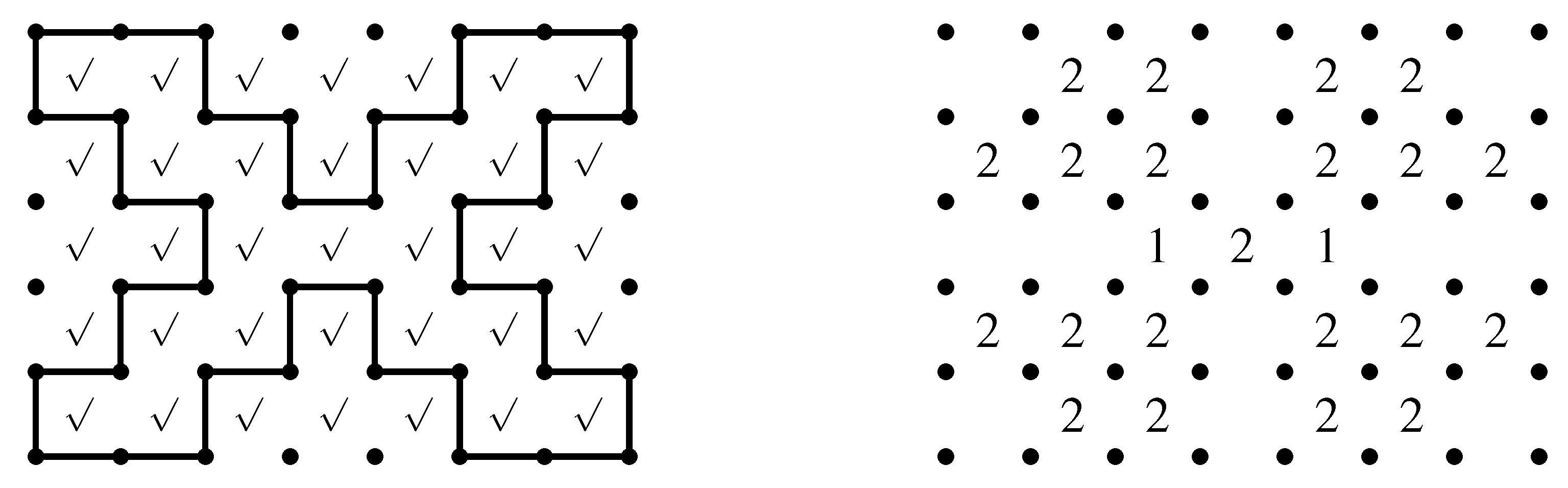
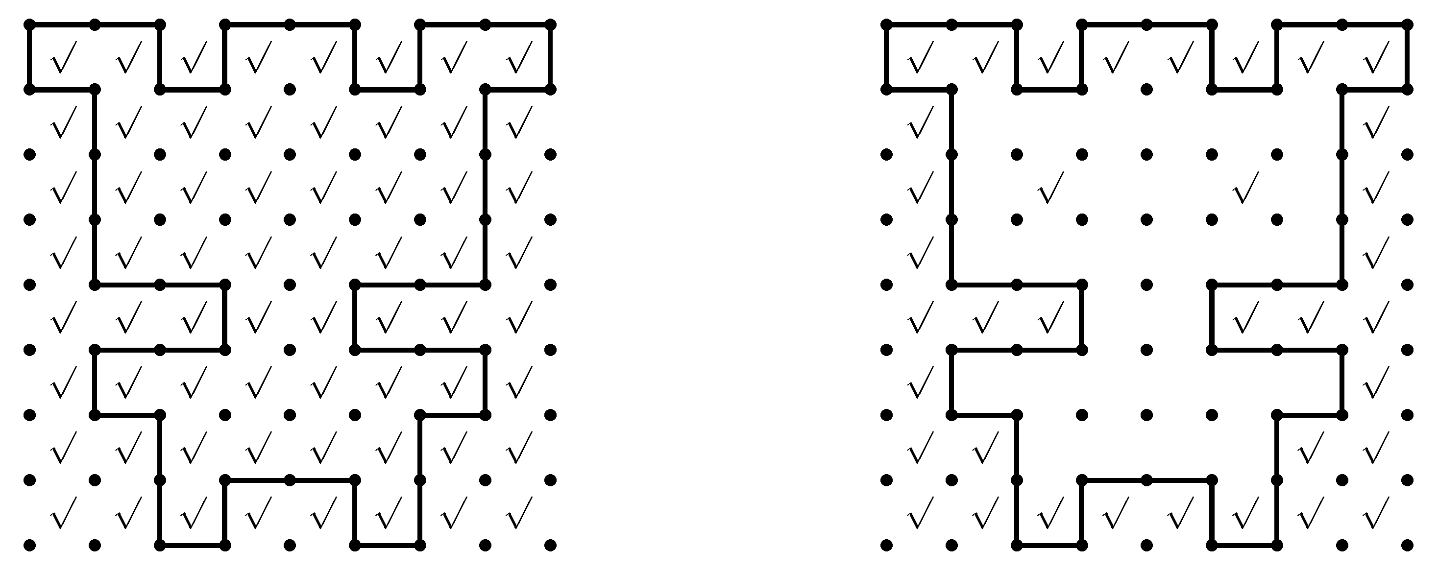
Figure 8 shows an example of Slitherlink generation. We drew a solution cycle on a grid of cells and marked all 35 cells as the maximum set of hint cells. When they were given as the input, our tool successfully constructed a ZDD for a family of sets of hint cells in 8 s, from which we can obtain all the 2,912,556,380 good Slitherlink instances that have the given solution cycle. The tool can optionally restrict generated instances to minimal ones (instances such that any hint cannot be removed without making the solution not unique). It took 0.1 s for this example and the number of instances was reduced to 32,639. The output example shown in Figure 8 is the one selected automatically by our tool as the most difficult instance among them in our criteria, in which the difficulty is evaluated by smallness of the number of cells with hint values “4”, “0”, “3”, “1”, and “2” in this order of precedence. Another output example was shown already in Figure 2, which is one of the 81 good instances that consist of minimum hints.
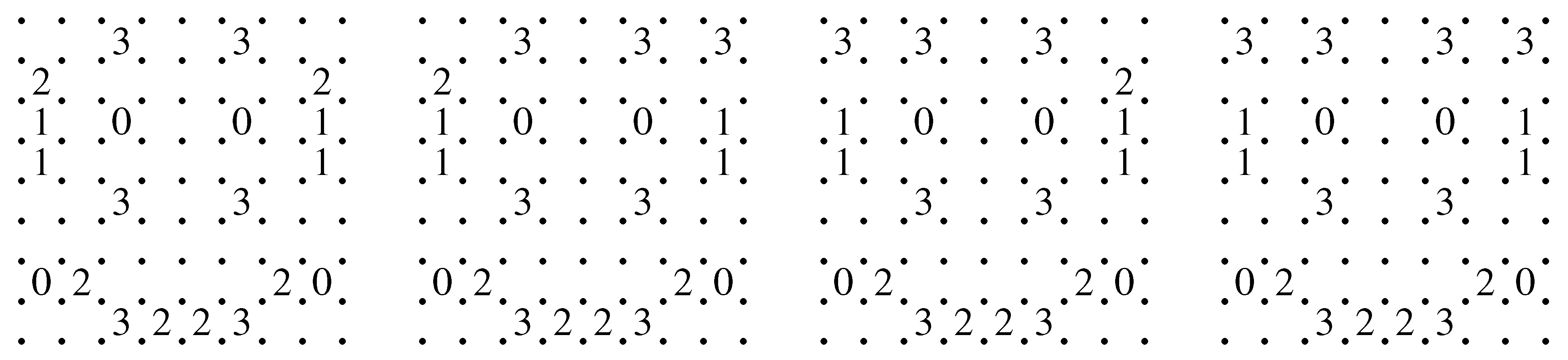
Figure 9 shows another input example, in which the solution cycle is drawn on a 8 × 8 grid of cells. Unfortunately, the computation could not be finished even in a day when all 64 cells are marked as candidates of hint locations. Our tool, however, was still able to assist making instances of the Slitherlink problem according to the designer’s intent. We reduced the candidate locations to 36 cells (the right picture of Figure 9) and got 1,669,424 instances, 1,850 minimal instances, and 4 minimum instances (Figure 10) in 2 s. It is also interesting that the same mechanism can be used to modify existing instances. We found that hand-made instances often include many redundant hints (e.g., 12 out of 40) and our tool can be used to make them more difficult to solve.
Finally, we introduce an enjoyable application of our tool, which can make a puzzle containing a secret message. Unlike the original Slitherlink, we allow multiple cycles as its solution in order to embed multiple letters into the puzzle. The algorithm of Slitherlink instance generation is modified by replacing computation of “all cycles on G” with “all combinations of disjoint cycles on G”, which is actually not difficult to be computed by using conditions on degree of the graph vertices. Figure 11 is our message to readers.
9. Conclusions
This paper has proposed algorithms that enumerate solutions and instances for two link puzzles, Numberlink and Slitherlink, based on Knuth’s path enumeration algorithm Simpath.
Our Numberlink solver (Algorithm 2) is faster than Sugar and CPLEX. In Slitherlink, our solution enumeration algorithm (Algorithm 5) shows better performance than Sugar. CPLEX is sometimes faster than our algorithm. Slink runs much faster than our algorithm and CPLEX to find a solution for Slitherlink instances. The result looks rather reasonable, since Sugar and CPLEX are designed for quite general purposes and find only one solution, while Slink is specially designed to solve Slitherlink problems. Our algorithms are located in between. The core of our algorithms is specialized to enumerate path matchings on a general graph, to which we have plugged mechanisms that decide whether the currently obtained path matchings can be expanded to a solution. It is not difficult to accelerate our algorithms by employing known local solution methods for the link puzzles on grid graphs. Yet we have largely ignored such detailed improvements. Rather we emphasize the generality of our approach that should be valid to design solution enumeration algorithms for various link puzzles including Masyu, Yajirin and others. To build a ZDD representing solutions, what we need to do is to assign each node an appropriate configuration like and which can be locally updated and which tells whether the currently obtained path matchings may be grown up to solutions.
Another point we would like to emphasize is that our algorithms give all the solutions at once as a ZDD unlike existing solvers. Our instance enumeration algorithms rely much on this feature of our approach. We benefit from the virtue of ZDDs as a set manipulation system. As we have demonstrated in Section 8.3, we have flexible means on ZDDs to extract instances with several properties from the whole set of good instances, like non-redundant ones, the hardest ones, ones that use specific cells, and so on. The authors believe manipulating puzzle instances on a ZDD is quite beneficial to puzzle designers. It is future work to develop an assistant tool for puzzle designers that equips several convenient functions with a friendly interface.
Acknowledgements
The authors are very much grateful to the anonymous reviewers for their valuable comments and suggestions that considerably improved the quality of our paper.
Appendix A Correctness of Algorithm 1 (Path Matching Enumeration)
This section proves that Algorithm 1 constructs a ZDD representing the family of path matchings over G. Hereafter refers to the function assigned to the node n by Algorithm 1 rather than the one given in Equation (2). Actually those two coincide as we will prove below.
For a -sequence of length i such that is a path matching, we define a mate function by
In the sequel, we assume that represents the special mate function whose domain is empty.
Lemma 8.
Let π be a -sequence of length . If is a path matching, then π is a valid path in and .
Proof.
We prove the lemma by induction on i. For , is the empty set, which is a special case of a path matching, and is the identity function on by definition. The empty path ends in the root node where we have .
Suppose that the lemma holds for of length where . If is a path matching, ends in a node in such that . By the algorithm, ends in a node such that
Suppose that is a path matching. Let consist of pairwise disjoint simple paths . Without loss of generality, we may assume that . We note that . Suppose that there are m distinct vertices such that . For each , we have
(Case 1) . Then consists of simple paths . By the assumption we have
Hence does not reject . Let be the 1-child of n. We have . Recall the definition of :
for all u in the domain of . Since and , the first case of the definition does not apply. The only vertices u such that are and . By the second case of the definition, we have and . Hence we obtain .
(Case 2) is a simple path. That is, either or . Without loss of generality, we assume . Since is not empty, . Then consists of simple paths . By the assumption we have
Hence does not reject . Also note that
if . Let be the 1-child of n, for which we have . By the definition of , we have
and for other vertices we have . The induction hypothesis implies .
(Case 3) is a path matching consisting of two simple paths and . That is, for some . Then consists of simple paths . By the assumption we have
Hence does not reject . Let be the 1-child of n, for which we have . By the definition of , we have
and for other vertices , we have . The induction hypothesis implies . □
Lemma 9.
Let π be a -sequence of length . If π ends in a node in , then is a path matching and .
Proof.
We show that if is not a path matching for a -sequence of length , then there is a prefix of such that ends in in .
Let be the longest prefix of such that is a path matching. Indeed such exists, since is a path matching for the empty sequence . Since is a path matching and so is , hence is a prefix of such that is not a path matching. By Lemma 8, is a valid path ending in a node n with . Let .
(Case 1) There exists a vertex v of degree more than 2 in . Since is a path matching, v has degree 2 in and . By Lemma 8, we have . Then rejects and ends in .
(Case 2) There exists no vertex of degree more than 2 in and there exists a simple cycle . Since is a path matching, we have and thus . There are distinct vertices for some such that and . Let , which is a simple path. Since has no vertex of degree more than 2, the degrees of and are 1 in . By and Lemma 8, we have and . Thus rejects and ends in . □
Theorem 10.
Algorithm 1 constructs a ZDD representing all the path matchings on G.
Proof.
By Lemmas 8 and 9. □
Appendix B Correctness of Algorithm 2 (Numberlink Solver)
Let denote the ZDD constructed by Algorithm 2 for input .
Lemma 11.
If a -sequence π ends in a node of , then is a path matching and .
Proof.
Obviously if is a valid path in , then it is also valid in . Moreover, Algorithms 1 and 2 assign the same mate function to the nodes reached by the same valid path . Thus the lemma follows from Lemma 8. □
Lemma 12
Let π be a -sequence of length such that is a path matching. If is incompatible with h, then there is no such that is a solution for .
Proof.
Suppose that is incompatible with h. Recall the definition that is incompatible with h if for some , either
- and , or
- and .
Accordingly we have two cases.
(Case 1) Suppose that there is such that . No edges incident to u belong to since . No edges incident to u belong to since. The vertex u has degree 0 in for any . Thus is not a solution, since .
(Case 2) Suppose that there is such that . The vertex has degree 1 in . No edges incident to u belong to by . The vertex has degree 1 in for any . Thus is not a solution, since . □
Lemma 13.
Let π be a -sequence of length such that is a path matching. If is incompatible with h, then there is no such that is a solution for .
Proof.
Suppose that is incompatible with h. Recall the definition that for , is incompatible with h if one of the following conditions holds.
- ,
- and ,
- and .
Let . Accordingly there are three cases.
(Case 1) Suppose that . In this case, it is easy to see that is not a path matching. Thus is not a solution for any .
(Case 2) Suppose that . If , then Case 1 applies. Otherwise, contains a v- path. Then v has degree 2 in . Thus is not a solution for any , since .
(Case 3) Suppose that , and . It is easy to see that has a - path. Let be such that is a path matching.
(Case 3.1) Suppose that . If , then has degree 2 in , which is not a solution. If , then contains a - path. Since , is not a solution.
(Case 3.2) Suppose that . Then contains a - path. Since , is not a solution. □
Corollary 14.
If is a solution for and , then π ends in in .
Proof.
For any prefix of length i of , is never incompatible with h by Lemmas 12 and 13. Together with Lemma 11, is a valid path in . □
Lemma 15.
Suppose that is not a solution for for a -sequence π of length . Then there are -sequences and such that for some and is incompatible with h.
Proof.
Suppose that is not a solution for . By the proofs of Lemmas 9 and 11, it is clear that if is not a path matching, then the lemma holds. We assume that is a path matching. We have the following cases.
- 1.
- contains a u-v path but , where
- 1.1.
- ,
- 1.2.
- and ,
- 1.3.
- .
- 2.
- does not contain a u-v path for some , where
- 2.1.
- u has degree 0,
- 2.2.
- u has degree 2,
- 2.3.
- u has degree 1.
Case 2.3 implies that contains a u-t path for some , which is covered by Cases 1.1 or 1.2. We discuss Cases 1.1, 1.2, 1.3, 2.1 and 2.2.
(Case 1.1) . Let P be the u-v path contained in and . Let be the prefix of length of and . Clearly is a prefix of . Let be such that and . We then have and . Thus is incompatible with h.
(Case 1.2) and . Let P be the u-v path contained in and where is the set of edges incident to v. We have by the choice of . Let be the prefix of length of and .
Suppose that . Then is a prefix of . Let be such that and . Thus , and , which means that is incompatible with h.
Suppose that . Then is a prefix of and contains the u-v path. We have and . That is, is incompatible with h.
(Case 1.3) . Let . We assume without loss of generality that for some . We have by the choice of . Let be the prefix of length of and .
Suppose that . For the edge in the u-v path incident to u, we have . Thus we have and , which means that is incompatible with h, where is a prefix of .
Suppose that . Then and is a prefix of . We have and . Hence is incompatible with h.
(Case 2.1) Suppose that has degree 0 in . Let and be the prefix of length of , where is a prefix of . Then and , which means that is incompatible with h,
(Case 2.2) Suppose that has degree 2 in . Let , be the prefix of length of , where is a prefix of . Then and , which means that is incompatible with h. □
Corollary 16.
If is not a solution for and , then π has a prefix which ends in in .
Proof.
By Lemmas 11 and 15. □
Appendix C Correctness of Algorithm 3 (Numberlink Instance Enumeration)
In this section, for a node n of , by and we denote the pair matching families assigned to n by Algorithm 3. For each -sequence such that is a path matching, let us define
Lemma 17.
Suppose that is a path matching and let and . We have
If is a path matching, then
Proof.
By definition,
and
□
Lemma 18.
For each node n of , the algorithm assigns . Moreover, for each.
Proof.
We show the lemma by induction on the length of . If is empty, then . Indeed Algorithm 3 sets .
Let for some and . By the induction hypothesis, we have . By Lemma 17, we have
We have proven that . and .
Conversely, we show by induction on i that if for , then there is such that and . For , and the empty path satisfies the claim. Suppose that for some with . Then by definition there is a b-parent of n for some such that . By definition, there is such that
By the induction hypothesis, there is such that and . Lemma 17 ensures that . This proves that and . □
Corollary 19. admits a solution if and only if .
Proof.
By Lemma 18. □
Lemma 20.
If for a -sequence π, then for each .
Proof.
Similarly to the proof of Lemma 18. □
Lemma 21.
If there are distinct valid paths and such that and , then .
Proof.
We prove the lemma by induction on . For , the claim holds since only the empty path ends in the root node.
Let and for some .
(Case 1) . In this case, we have and . Let and . Clearly each of has the same degree in and in , since u and v are in the domain of . To derive a contradiction, suppose that , where we assume without loss of generality that and . Then u has different degrees in and in . In this case, the fact that implies that u is not in the domain of those mate functions. The same argument applies to v. Hence, by definition. The fact that is a path matching implies , which means that does not contain a u-v path. Hence does not have a - path and . This contradicts to the assumption that . Hence we conclude that . By Lemma 17, we have
Together with , and , we conclude that . By , we have . By the induction hypothesis, . Thus by Lemma 20, .
(Case 2) . By Lemma 18, we have and . Hence . □
Lemma 22.
For any valid path π such that , it holds that .
Proof.
We prove the lemma by induction on . For , the claim holds trivially by . Let for some .
(Case 1) . We have
By the induction hypothesis, we have . Hence .
(Case 2) . The fact implies that . Let . We have . By Lemma 18 and the fact , we have
□
Lemma 23.
If for some node in , then one of the following holds:
- there are distinct and such that and ,
- there is π such that , and .
Proof.
We prove the lemma by induction on i such that . For , the claim holds trivially by .
For , there are three cases according to the definition of in the algorithm.
(Case 1) for some -parents of n for such that . By Lemma 18, there are such that and for . The fact implies that . We have and .
(Case 2) for some 0-parent of n such that for some . By Lemma 18, there is such that and . The fact that implies that the degree of u is 0 in . Let . Then, we have , and .
(Case 3) for some b-parent of n. There is such that . By the induction hypothesis on the fact , one of the following holds:
- there are distinct and such that and ,
- there is such that , and .
In the former case, for satisfies the lemma. In the latter case, let . By , we have . Thus we have for . □
Appendix D Correctness of Algorithm 4 (Cycle Enumeration)
Let be the output by Algorithm 4 for G. The following lemma, which we will use without explicit reference, is implied by the proof of Lemma 8.
Lemma 24.
If π is a valid path in and , then is a path matching and .
For , we have the following stronger lemma.
Lemma 25.
Let π be a -sequence of length at most . If is a path matching such that every vertex in has degree 0 or 2 in , then π is a valid path ending in a node in the constructed ZDD and we have .
Proof.
We prove the lemma by induction on the length of . Clearly the lemma holds if is the empty sequence. Suppose that of length satisfies the condition of the lemma. Let . It is enough to show the following by Lemma 24.
- If has a fixed end, then there is a vertex in of degree 1 in .
- If is a path matching and has a fixed end, then there is a vertex in of degree 1 in .
Suppose that has a fixed end. By definition, there is with , which means that v has degree 1 in .
Suppose that is a path matching and has a fixed end. By definition, there is with , which means that v has degree 1 in by the arguments on the function in the proof of Lemma 8. □
Corollary 26.
Let π be a -sequence of length . If is a simple cycle, then ends in .
Proof.
Suppose that is a cycle. Let and . That is, . Since is a u-v simple path, the only vertices of degree 1 in are u and v. Since , Lemma 25 implies that ends in a node . We have , and for other . That is, and form a cycle. The algorithm connects n and by a 1-arc. □
Lemma 27.
Let π be a -sequence of length . If π ends in a node , then is a path matching such that and every vertex in has degree 0 or 2 in .
Proof.
We show the lemma by induction on i. A proof almost identical to that for Lemma 9 applies to the claim that if ends in a node , then is a path matching such that . We here show that in that case every vertex in has degree 0 or 2 in .
If is empty, then is the empty set.
Suppose that for some . We have . By the induction hypothesis, every vertex in has degree 0 or 2 in where . If , there is nothing to prove. If there is , then . By definition, does not have a fixed end, i.e., . That is, u has degree 0 or 2.
The case where for some can be proven by combining the discussions for the case where and the correctness of the mate updating function , established in the proof of Lemma 8. □
Corollary 28.
If a -sequence π ends in , then is a simple cycle.
Proof.
By the algorithm, must have the form and and form a cycle for . That is, we have
Applying Lemma 27 to , we conclude that is a path matching consisting solely of a u-v path for . Clearly is a simple cycle. □
Theorem 29.
Algorithm 4 constructs a ZDD that represents all the simple cycles on G.
Proof.
By Corollaries 26 and 28. □
Appendix E Correctness of Algorithm 5 (Slitherlink Solver)
Let be the output by Algorithm 5 for .
Lemma 30.
If a -sequence π ends in in , then is a solution for .
Proof.
By Lemma 27, If ends in a node , then is a path matching such that every vertex in has degree 0 or 2 in and . Moreover, it is easy to show by induction on i that for all .
If ends in , by definition of , is a cycle such that for all . That is, is a solution for . □
Lemma 31.
If a -sequence π of length i ends in in , then is not a solution for for any .
Proof.
Suppose that ends in where . Let , and
for all . The proof of Lemma 25 shows that if has a fixed end or declines , then the lemma holds. It is enough to discuss the case where is incompatible with h. In this case, either or for some . In the former case, implies that for any . That is, cannot be a solution. In the latter case,
implies that for any . That is, cannot be a solution. □
Corollary 32.
represents the set of all solutions for .
Proof.
By Lemmas 30 and 31. □
Appendix F Computation Example for Numberlink Instance Enumeration
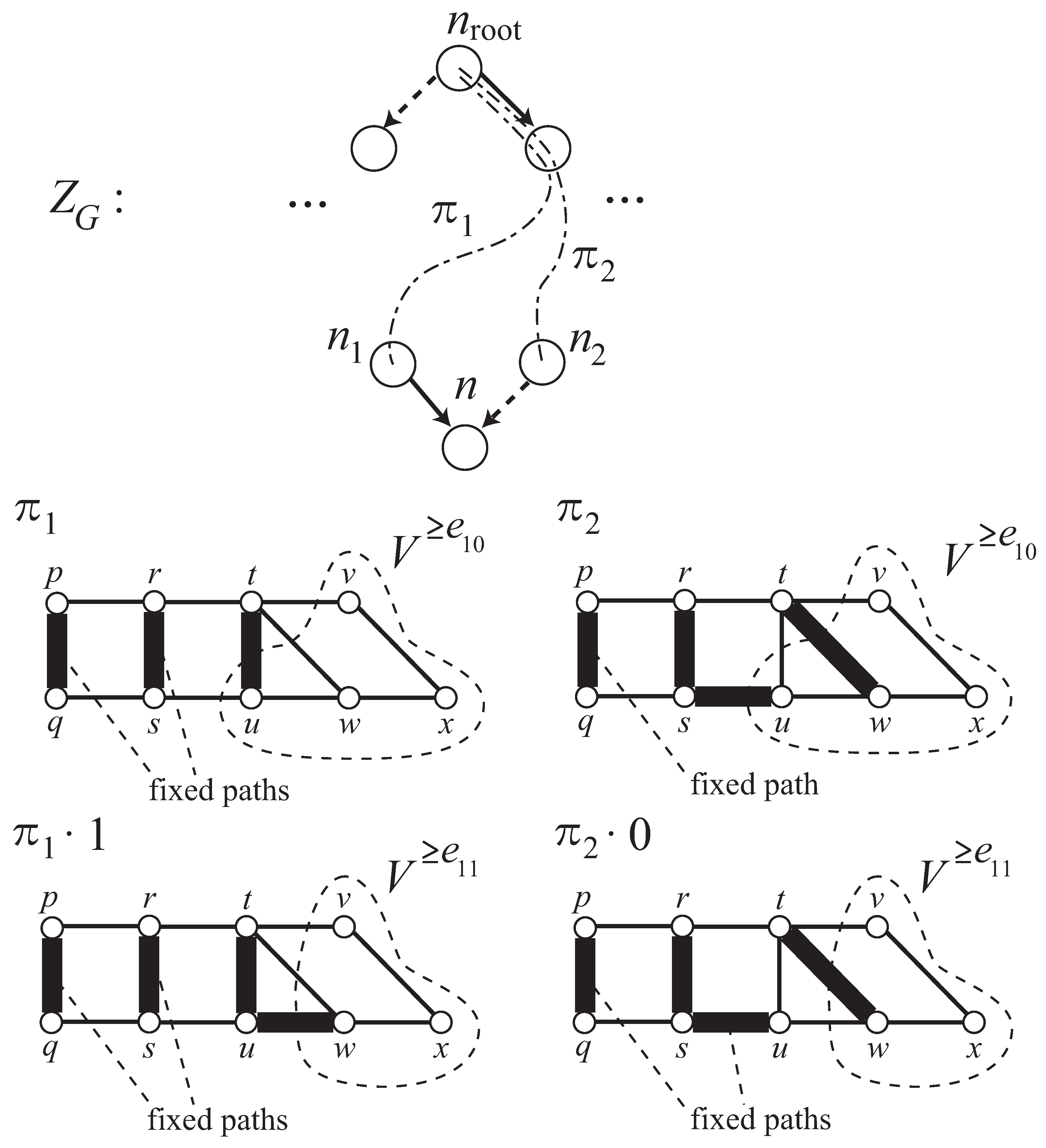
We explain an example of and for some valid path and some node n defined in Section 5 (see Figure 12).
Figure 12.
An example of computing T(π) and Sn.


A given graph and are shown in the top half of the figure. The dashed lines represent valid paths and . The four graphs in the bottom half of the figure are subgraphs whose vertex sets are V and whose edge sets are , , and , which are drawn as bold lines. Since , and and for any other vertices u, both and are undefined, holds. Therefore, . Let . Let , and . , , and include two fixed paths and , one fixed path , two fixed paths and , and two fixed paths and respectively. It is easy to verify that , , and hold.
Appendix G Minimum Good Numberlink Instances over G 6,6
Figure 13.
Good instances on (1).

Figure 14.
Good instances on (2).

References
- Nikoli: Web Nikoli. Available online: http://www.nikoli.co.jp/ (accessed on 21 March 2012).
- Kotsuma, K.; Takenaga, Y. NP-Completeness and Enumeration of Number Link Puzzle [in Japanese]; IEICE Technical Report, COMP2009-49; The Institute of Electronics, Information and Communication Engineering: Tokyo, Japan, 2010; pp. 1–7. [Google Scholar]
- Kramer, M.R.; van Leeuwen, J. Wire-Routing is NP-Complete; Report No. RUU-CS-82-4; Department of Computer Science, University of Utrecht: Utrecht, The Netherlands, 1982. [Google Scholar]
- Takahashi, J.; Suzuki, H.; Nishizeki, T. Shortest noncrossing paths in plane graphs. Algorithmica 1996, 16, 339–357. [Google Scholar] [CrossRef]
- Richards, D. Complexity of single-layer routing. IEEE Trans. Comput. 1984, 33, 286–288. [Google Scholar] [CrossRef]
- Yato, T. On the NP-Completeness of the Slither Link Puzzle [in Japanese]; IPSJ SIG Notes AL-74; Information Processing Society of Japan: Tokyo, Japan, 2000; pp. 25–32. [Google Scholar]
- Hearn, R.A.; Demaine, E.D. Games, Puzzles, and Computation; A K Peters, Ltd.: Boca Raton, FL, USA, 2009. [Google Scholar]
- Tamura, N. Sugar: A SAT-Based Constraint Solver. Available online: http://bach.istc.kobe-u.ac.jp/ sugar/ (accessed on 21 March 2012).
- Itogawa, A. Slither Link Kaito Program (Solving Slither Link Program: In Japanese). Available online: http://www2.ttcn.ne.jp/~itogawa/product/slitherlink.html (accessed on 21 March 2012).
- Shirai, H.; Igarashi, C.; Tajima, Y.; Kotani, Y. Solving and Making Problems of Slither Link [in Japanese]. In Proceedings of the 11th Game Programming Workshop in Japan 2006, Kanagawa, Japan, 10–12 November 2006; pp. 32–39. [Google Scholar]
- Wan, J. Logical Slither Link. Bsc These, University of Manchester, Manchester, UK, 2009. [Google Scholar]
- Minato, S. Zero-Suppressed BDDs for Set Manipulation in Combinatorial Problems. In Proceedings of the 30th International Design Automation Conference (DAC ’93), Dallas, TX, USA, 14–18 June 1993; pp. 272–277. [Google Scholar]
- Knuth, D. The Art of Computer Programming, Volume 4, Fascicle 1; Addison-Wesley Professional: Boston, MA, USA, 2009. [Google Scholar]
- Yato, T.; Seta, T. Complexity and completeness of finding another solution and its application to puzzles. IEICE Trans. Fundam. Electron. Commun. Comput. Sci. 2003, E86-A, 1052–1060. [Google Scholar]
- GLPK deno Pencil Puzzle Koryakuho (Solving Pencil Puzzle Using GLPK : In Japanese). Available online: http://www21.tok2.com/home/kainaga11/glpk/glpk.htm (accessed on 21 March 2012).
- Sugimura, Y. Seisu Keikakuho niyoru Slither Link no Kaiho (Slither Link Algorithm Using Integer Programming: In Japanese). In Proceedings of the 1st Games and Puzzles Mini Workshop, Kyoto, Japan, 12 September 2005. [Google Scholar]
- Tamura, N. Solving Number Link Puzzles with Sugar Constraint Solver [in Japanese]. Available online: http://bach.istc.kobe-u.ac.jp/sugar/puzzles/numberlink.html (accessed on 21 March 2012).
- Tamura, N. Solving Slither Link Puzzles with Sugar Constraint Solver [in Japanese]. Available online: http://bach.istc.kobe-u.ac.jp/sugar/puzzles/slitherlink.html (accessed on 21 March 2012).
- Nikoli. Numberlink 1; Nikoli: Tokyo, Japan, 1989. [Google Scholar]
- Nikoli: Nikoli.com Puzzle Championship. Available online: http://www.nikoli.com/en/event/ puzzle_hayatoki.html (accessed on 21 March 2012).
- Nikoli. Slitherlink 1; Nikoli: Tokyo, Japan, 1992. [Google Scholar]
- Nikoli: Sample Problems of Slitherlink Puzzle. Available online: http://www.nikoli.com/en/ puzzles/slitherlink/ (accessed on 21 March 2012).
Figure 1.
An instance of Numberlink and its solution.

Figure 2.
An instance of Slitherlink and its solution.

Figure 3.
The reduced ZDD representing . where . Dotted lines represent 0-arcs and solid lines represent 1-arcs.
Figure 3.
The reduced ZDD representing . where . Dotted lines represent 0-arcs and solid lines represent 1-arcs.

Figure 4.
An example of G and .

Figure 5.
updating mate.

Figure 6.
Grid graph and its vertex labels.

Figure 7.
An example of information used by a heuristic Slitherlink solver.

Figure 8.
Input and output of Slitherlink generation; example #1.

Figure 9.
Input of Slitherlink generation; example #2.

Figure 10.
Output of Slitherlink generation; example #2.

Figure 11.
An example of message puzzle instance.


Table 1.
Running time in seconds for solving Numberlink. Our algorithm could not solve C88 due to insufficient memory.
Table 1.
Running time in seconds for solving Numberlink. Our algorithm could not solve C88 due to insufficient memory.
| Instance | Graph | Time CPLEX | Time Sugar | Time Algorithm 2 | Memory Algorithm 2 (MB) |
|---|---|---|---|---|---|
| BN1 | 0.02 | 1.179 | 0.008 | 2 | |
| BN15 | 13.95 | 1.336 | 0.004 | 2 | |
| BN30 | 88.32 | 1.896 | 0.016 | 5 | |
| BN43 | 6,410.67 | 1.924 | 0.072 | 18 | |
| BN52 | 0.45 | 1.520 | 0.012 | 3 | |
| BN64 | 108.07 | 1.704 | 0.136 | 11 | |
| BN72 | 276.07 | 1.388 | 0.012 | 4 | |
| BN79 | 15,117.47 | 1.496 | 0.220 | 37 | |
| BN85 | >100,000 | 7,213.079 | 862.518 | 43,846 | |
| BN99 | >100,000 | 14.097 | 1,658.772 | 67,094 | |
| C88 | >100,000 | >100,000 |
Table 2.
Running time in seconds for solving Numberlink with restriction that requires solutions to cover all vertices.
Table 2.
Running time in seconds for solving Numberlink with restriction that requires solutions to cover all vertices.
| Instance | Graph | Time CPLEX | Time Sugar | Time Algorithm 2 | Memory Algorithm 2 (MB) |
|---|---|---|---|---|---|
| BN1 | 0.01 | 1.148 | 0.004 | 2 | |
| BN15 | 0.40 | 0.964 | 0.000 | 2 | |
| BN30 | 0.82 | 1.576 | 0.024 | 3 | |
| BN43 | 21.97 | 1.552 | 0.012 | 5 | |
| BN52 | 0.10 | 1.296 | 0.004 | 2 | |
| BN64 | 18.40 | 1.368 | 0.012 | 5 | |
| BN72 | 1.50 | 1.648 | 0.012 | 2 | |
| BN79 | 26.74 | 1.452 | 0.048 | 10 | |
| BN85 | >100,000 | 5,431.991 | 185.264 | 8,761 | |
| BN99 | >100,000 | 12.585 | 175.147 | 9,727 |
Table 3.
Running time in seconds for solving Slitherlink. Our algorithm could not solve C95 due to insufficient memory.
Table 3.
Running time in seconds for solving Slitherlink. Our algorithm could not solve C95 due to insufficient memory.
| Instance | Graph | Time CPLEX | Time Sugar | Time slink | Time Algorithm 5 | Memory Algorithm 5 (MB) |
|---|---|---|---|---|---|---|
| BS1 | 0.07 | 5.460 | 0.001 | 0.116 | 34 | |
| BS12 | 0.28 | 4.696 | 0.004 | 0.384 | 41 | |
| BS25 | 0.12 | 6.496 | 0.001 | 0.060 | 34 | |
| BS37 | 0.14 | 8.773 | 0.004 | 0.044 | 34 | |
| BS43 | 0.17 | 8.349 | 0.001 | 0.060 | 36 | |
| BS54 | 0.40 | 7.380 | 0.008 | 0.304 | 37 | |
| BS68 | 0.39 | 12.433 | 0.004 | 0.384 | 39 | |
| BS77 | 0.90 | 13.281 | 0.004 | 0.376 | 42 | |
| BS89 | 1.56 | 48.035 | 0.016 | 9.329 | 407 | |
| BS96 | 3.07 | 186.612 | 0.104 | 26.286 | 904 | |
| S10 | 41.43 | 1,411.944 | 0.036 | 4,569.330 | 138,053 | |
| C95 | 95.93 | 1,076.839 | 0.088 |
Table 4.
Running time of Numberlink generator for .
| 2 | 3 | 4 | 5 | 6 | 7 | |
|---|---|---|---|---|---|---|
| 2 | <0.01 | <0.01 | <0.01 | <0.01 | 0.01 | 0.02 |
| 3 | <0.01 | 0.01 | 0.08 | 0.48 | 2.67 | |
| 4 | 0.21 | 3.56 | 44.13 | 488.12 | ||
| 5 | 107.99 | 3,553.29 | >100,000 | |||
| 6 | >100,000 | >100,000 | ||||
| 7 | >100,000 |
Table 5.
The number of good instances of Numberlink for .
| 2 | 3 | 4 | 5 | 6 | 7 | |
|---|---|---|---|---|---|---|
| 2 | 2 | 10 | 36 | 126 | 454 | 1,632 |
| 3 | – | 86 | 807 | 6,690 | 58,422 | 499,733 |
| 4 | – | – | 16,410 | 338,460 | 6,901,105 | 141,123,690 |
| 5 | – | – | – | 16,027,290 | 784,030,205 | Time Out |
| 6 | – | – | – | – | Time Out | Time Out |
| 7 | – | – | – | – | – | Time Out |
Table 6.
The number of ZDD nodes of in Numberlink generator for .
| 2 | 3 | 4 | 5 | 6 | 7 | |
|---|---|---|---|---|---|---|
| 2 | 4 | 18 | 50 | 117 | 235 | 419 |
| 3 | – | 99 | 491 | 1,686 | 4,918 | 12,255 |
| 4 | – | – | 3,499 | 22,599 | 108,954 | 439,506 |
| 5 | – | – | – | 226,800 | 1,977,335 | Time Out |
| 6 | – | – | – | – | Time Out | Time Out |
| 7 | – | – | – | – | – | Time Out |
Table 7.
Running time, the number of good instances with at most ℓ pairs of numbers, and that of ZDD nodes of .
Table 7.
Running time, the number of good instances with at most ℓ pairs of numbers, and that of ZDD nodes of .
| Graph | ℓ | Time | Good instances | |
|---|---|---|---|---|
| 0 | 39.63 | 0 | 1 | |
| 1 | 141.13 | 0 | 1 | |
| 2 | 1,329.35 | 0 | 1 | |
| 3 | 12,161.5 | 304 | 472 | |
| 4 | >1,000,000 | |||
| 0 | 2,732.86 | 0 | 1 | |
| 1 | 14,226 | 0 | 1 | |
| 2 | >1,000,000 |
Publisher’s Note: MDPI stays neutral with regard to jurisdictional claims in published maps and institutional affiliations. |
© 2012 by the authors. Licensee MDPI, Basel, Switzerland. This article is an open access article distributed under the terms and conditions of the Creative Commons Attribution (CC BY) license (https://creativecommons.org/licenses/by/4.0/).
Share and Cite
MDPI and ACS Style
Yoshinaka, R.; Saitoh, T.; Kawahara, J.; Tsuruma, K.; Iwashita, H.; Minato, S.-i. Finding All Solutions and Instances of Numberlink and Slitherlink by ZDDs. Algorithms 2012, 5, 176-213. https://0-doi-org.brum.beds.ac.uk/10.3390/a5020176
AMA Style
Yoshinaka R, Saitoh T, Kawahara J, Tsuruma K, Iwashita H, Minato S-i. Finding All Solutions and Instances of Numberlink and Slitherlink by ZDDs. Algorithms. 2012; 5(2):176-213. https://0-doi-org.brum.beds.ac.uk/10.3390/a5020176
Chicago/Turabian StyleYoshinaka, Ryo, Toshiki Saitoh, Jun Kawahara, Koji Tsuruma, Hiroaki Iwashita, and Shin-ichi Minato. 2012. "Finding All Solutions and Instances of Numberlink and Slitherlink by ZDDs" Algorithms 5, no. 2: 176-213. https://0-doi-org.brum.beds.ac.uk/10.3390/a5020176