Pattern-Guided k-Anonymity

Institut für Softwaretechnik und Theoretische Informatik, TU Berlin, Berlin, 10587, Germany
*
Author to whom correspondence should be addressed.
Algorithms 2013, 6(4), 678-701; https://0-doi-org.brum.beds.ac.uk/10.3390/a6040678
Submission received: 2 August 2013
/
Revised: 9 October 2013
/
Accepted: 9 October 2013
/
Published: 17 October 2013
Abstract
:We suggest a user-oriented approach to combinatorial data anonymization. A data matrix is called k-anonymous if every row appears at least k times—the goal of the NP-hard k-Anonymity problem then is to make a given matrix k-anonymous by suppressing (blanking out) as few entries as possible. Building on previous work and coping with corresponding deficiencies, we describe an enhanced k-anonymization problem called Pattern-Guided k-Anonymity, where the users specify in which combinations suppressions may occur. In this way, the user of the anonymized data can express the differing importance of various data features. We show that Pattern-Guided k-Anonymity is NP-hard. We complement this by a fixed-parameter tractability result based on a “data-driven parameterization” and, based on this, develop an exact integer linear program (ILP)-based solution method, as well as a simple, but very effective, greedy heuristic. Experiments on several real-world datasets show that our heuristic easily matches up to the established “Mondrian” algorithm for k-Anonymity in terms of the quality of the anonymization and outperforms it in terms of running time.
1. Introduction
Making a matrix k-anonymous, that is, each row has to occur at least k times, is a classic model for (combinatorial) data privacy [1,2]. We omit considerations on the also very popular model of “differential privacy” [3], which has a more statistical than a combinatorial flavor. It is well-known that there are certain weaknesses of the k-anonymity concept, for example, when the anonymized data is used multiple times [1]. Here, we focus on k-anonymity, which, due to its simplicity and good interpretability, continues to be of interest in current applications. The idea behind k-anonymity is that each row of the matrix represents an individual, and the k-fold appearance of the corresponding row shall avoid the situation in which the person or object behind can be identified. To reach this goal, clearly, some information loss has to be accepted, that is, some entries of the matrix have to be suppressed (blanked out); in this way, information about certain attributes (represented by the columns of the matrix) is lost. Thus, the natural goal is to minimize this loss of information when transforming an arbitrary data matrix into a k-anonymous one. The corresponding optimization problem k-Anonymity is NP-hard (even in special cases) and hard to approximate [4,5,6,7,8]. Nevertheless, it played a significant role in many applications, thereby mostly relying on heuristic approaches for making a matrix k-anonymous [2,9,10].
It was observed that care has to be taken concerning the “usefulness” (also in terms of expressiveness) of the anonymized data [11,12]. Indeed, depending on the application that has to work on the k-anonymized data, certain entry suppressions may “hurt” less than others. For instance, considering medical data records, the information about eye color may be less informative than information about blood pressure. Hence, it would be useful for the user of the anonymized data to specify information that may help in doing the anonymization process in a more sophisticated way. Thus, in recent work [13], we proposed a “pattern-guided” approach to data anonymization, in a way that allows the user to specify which combinations of attributes are less harmful to suppress than others. More specifically, the approach allows “pattern vectors”, which may be considered as blueprints for the structure of anonymized rows—each row has to be matched with exactly one of the pattern vectors (we will become more precise about this when formally introducing our new model). The corresponding proposed optimization problem [13], however, has the clear weakness that each pattern vector can only be used once, disallowing that there are different incarnations of the very same anonymization pattern. While this might be useful for the clustering perspective of the problem [13], we see no reason to justify this constraint from the viewpoint of data privacy. This leads us to proposing a modified model, whose usefulness for practical data anonymization tasks is supported by experiments on real-world data and comparison with a known k-anonymization algorithm.
Altogether, with our new model, we can improve both on k-Anonymity by letting the data user influence the anonymization process, as well as on the previous model [13] by allowing full flexibility for the data user to influence the anonymization process. Notably, the previous model is more suitable for homogeneous team formation instead of data anonymization [14].
An extended abstract of this work appeared in the Proceedings of the Joint Conference of the 7th International Frontiers of Algorithmics Workshop and the 9th International Conference on Algorithmic Aspects of Information and Management (FAW-AAIM ’13), Dalian, China, Volume 7924, of Lecture Notes in Computer Science, pages 350–361, June, 2013. © Springer. This full version contains all proof details and an extended experimental section. Furthermore, we provide the new result that Pattern-Guided 2-Anonymity is polynomial-time solvable (Theorem 2).
Formal Introduction of the New Model.
A row type is a maximal set of identical rows of a matrix.
Matrices are made k-anonymous by suppressing some of their entries. Formally, suppressing an entry of an -matrix M over alphabet Σ with and means to simply replace by the new symbol “☆”, ending up with a matrix over the alphabet .
Our central enhancement of the k-Anonymity model lies in the user-specific pattern mask guiding the anonymization process: Every row in the k-anonymous output matrix has to conform to one of the given pattern vectors. Note that both the input table and the given patterns mathematically are matrices, but we use different terms to more easily distinguish between them: the “pattern mask” consists of “pattern vectors”, and the “input matrix” consists of “rows”.
Definition 2.
A row r in a matrix matches a pattern vector if and only if that is, r and v have ☆-symbols at the same positions.
With these definitions, we can now formally define our central computational problem. The decisive difference with respect to our previous model [13] is that in our new model, two non-identical output rows can match the same pattern vector.
Pattern-Guided k-Anonymity
| Input: | A matrix , a pattern mask , and two positive integers k and s. |
| Question: | Can one suppress at most s entries of M in order to obtain a k-anonymous matrix , such that each row type of matches to at least one pattern vector of P? |
For some concrete examples, we refer to Section 3.6.
Our Results Describing a polynomial-time many-to-one reduction from the NP-hard 3-Set Cover problem, we show that Pattern-Guided k-Anonymity is NP-complete; even if the input matrix only consists of three columns, there are only two pattern vectors, and . Motivated by this computational intractability result, we develop an exact algorithm that solves Pattern-Guided k-Anonymity in time for an input matrix M, p pattern vectors, and the number of different rows in M being t. In other words, this shows that Pattern-Guided k-Anonymity is fixed-parameter tractable for the combined parameter and actually can be solved in linear time if t and p take constant values. (The fundamental idea behind parameterized complexity analysis [18,19,20] is, given a computationally hard problem Q to identify a parameter ℓ (typically, a positive integer or a tuple of positive integers), for Q and to determine whether size-s instances of Q can be solved in time, where f is an arbitrary computable function.) This result appears to be of practical interest only in special cases (“small” values for t and p are needed). It nevertheless paves the way for a formulation of an integer linear program for Pattern-Guided k-Anonymity that exactly solves moderate-size instances of Pattern-Guided k-Anonymity in reasonable time. Furthermore, our fixed-parameter tractability result also leads to a simple and efficient greedy heuristic, whose practical competitiveness is underlined by a set of experiments with real-world data, also favorably comparing with the Mondrian algorithm for k-Anonymity [21]. In particular, our empirical findings strongly indicate that, even when neglecting the aspect of potentially stronger expressiveness on the data user side provided by Pattern-Guided k-Anonymity, in combination with the greedy algorithm, it allows for high-quality and very fast data anonymization, being comparable in terms of anonymization quality with the established Mondrian algorithm [21], but significantly outperforming it in terms of time efficiency.
2. Complexity and Algorithms
This section is organized as follows. In Section 2.1, we prove the NP-hardness of Pattern-Guided 3-Anonymity restricted to two pattern vectors and three columns. To complement this intractability result, we also present a polynomial-time algorithm for Pattern-Guided 2-Anonymity and a fixed-parameter algorithm for Pattern-Guided k-Anonymity. In Section 2.2 and Section 2.3, we extract the basic ideas of the fixed-parameter algorithm for an integer linear program (ILP) formulation and a greedy heuristic.
2.1. Parameterized Complexity
One of the decisions made when developing fixed-parameter algorithms is the choice of the parameter. Natural parameters occurring in the problem definition of Pattern-Guided k-Anonymity are the number n of rows, the number m of columns, the alphabet size , the number p of pattern vectors, the anonymity degree k, and the cost bound s. In general, the number of rows will arguably be large and, thus, also the cost bound s, tends to be large. Since fixed-parameter algorithms are fast when the parameter is small, trying to exploit these two parameters tends to be of little use in realistic scenarios. However, analyzing the adult dataset [22] prepared as described by Machanavajjhala et al. [23], it turns out that some of the other mentioned parameters are small: The dataset has columns, and the alphabet size is 73. Furthermore, it is natural to assume that also the number of pattern vectors is not that large. Indeed, compared to the rows, even the number of all possible pattern vectors is relatively small. Finally, there are applications where k, the degree of anonymity, is small [24]. Summarizing, we can state that fixed-parameter tractability with respect to the parameters , m, k, or p, could be of practical relevance. Unfortunately, by reducing from 3-Set Cover, we can show that Pattern-Guided k-Anonymity is NP-hard in very restricted cases.
Theorem 1.
Pattern-Guided k-Anonymity is NP-complete even for two pattern vectors, three columns, and .
Proof. We reduce from the NP-hard 3-Set Cover [25]: Given a set family with over a universe and a positive integer h, the task is to decide whether there is a subfamily of size at most h such that . In the reduction, we need unique entries in the constructed input matrix M. For ease of notation, we introduce the ▵-symbol with an unusual semantics. Each occurrence of a ▵-symbol stands for a different unique symbol in the alphabet Σ. One could informally state this as “”. We now describe the construction. Let be the 3-Set Cover instance. We construct an equivalent instance of Pattern-Guided k-Anonymity as follows: Initialize M and P as empty matrices. Then, for each element , add the row twice to the input matrix M. For each set with , add to M the three rows , , and . Finally, set , , and add to P the pattern vectors (□, ☆, ☆), and (☆, □, □).
We show the correctness of the above construction by proving that is a yes-instance of 3-Set Cover, if and only if is a yes-instance of Pattern-Guided k-Anonymity.
“⇒:” If is a yes-instance of 3-Set Cover, then there exists a set cover of size at most h. We suppress the following elements in M: First, suppress all ▵-entries in M. This gives suppressions. Then, for each , suppress all -entries in M. This gives suppressions. Finally, for each , suppress the first column of all rows containing the entry . These are suppressions. Let denote the matrix with the suppressed elements. Note that contains suppressed entries. Furthermore, in each row in , either the first element is suppressed or the last two elements. Hence, each row of matches to one of the two pattern vectors of P. Finally, observe that is 3-anonymous: The three rows corresponding to the set are identical: the first column is suppressed, and the next two columns contain the symbol . Since is a set cover, there exists for each element a set such that . Thus, by construction, the two rows corresponding to the element , and the row in M coincide in : The first column contains the entry and the other two columns are suppressed. Finally, for each row in M that corresponds to a set , the row in coincides with the two rows corresponding to the element : Again, the first column contains the entry and the other two columns are suppressed.
“⇐:” If is a yes-instance of Pattern-Guided k-Anonymity, then there is a 3-anonymous matrix , that is obtained from M by suppressing at most s elements, and each row of matches to one of the two pattern vectors in P. Since M and, so, contain rows, contains at most suppressions and each pattern vector contains a ☆-symbol, there are at most rows in containing two suppressions and at least rows containing one suppression. Furthermore, since the rows in M corresponding to the elements of U contain the unique symbol ▵ in the last two columns in , these rows are suppressed in the last two columns. Thus, at most rows corresponding to sets of have two suppressions in . Observe that for each set the entries in the last two columns of the corresponding rows are . There is no other occurrence of this entry in M. Hence, the at least rows in with one suppression correspond to sets in . Thus, the at most rows in that correspond to sets of and contain two suppressions correspond to at most h sets of . Denote these h sets by . We now show that is a set cover for the 3-Set Cover instance. Assume by contradiction that is not a set cover, and hence, there is an element . However, since is 3-anonymous, there has to be a row r in that corresponds to some set such that this row coincides with the two rows and corresponding to u. Since all rows in corresponding to elements of U contain two suppressions in the last two columns, the row r also contains two suppressions in the last two columns. Thus, . Furthermore, r has to coincide with and in the first column, that is, r contains as the entry in the first column the symbol u. Hence, , a contradiction. ☐
Blocki and Williams [7] showed that, while 3-Anonymity is NP-complete [7,8], 2-Anonymity is polynomial-time solvable by reducing it in polynomial time to the polynomial-time solvable, Simplex Matching [26], defined as follows:
Simplex Matching
- Input:
- A hypergraph with hyperedges of size two and three, a positive integer h, and a cost function, , such that:
- and
- .
- Question:
- Is there a subset of the hyperedges , such that for all , there is exactly one edge in containing v and ?
We slightly adjust their reduction to obtain polynomial-time solvability for Pattern-Guided 2-Anonymity, together with Theorem 1, yielding a complexity dichotomy for Pattern-Guided k-Anonymity with respect to the parameter k.
Theorem 2. Pattern-Guided 2-Anonymity is polynomial-time solvable.
Proof. We reduce Pattern-Guided 2-Anonymity to Simplex Matching. To this end, we first introduce some notation. Let be the Pattern-Guided 2-Anonymity instance. For a set A of rows and a pattern vector p in P the set is obtained from A by suppressing entries in the rows of A such that each row matches p (see Definition 2). The set contains all pattern vectors p such that is a set of identical rows. Intuitively, contains all “suitable” pattern vectors to make the rows in A identical.
Now, construct the hypergraph as follows: Initialize and . For each row r in M add a vertex to V. For a vertex subset let be the set of the corresponding rows in M. For each vertex subset of size add the hyperedge if . Let be a pattern vector in with the minimum number of ☆-symbols. Denote this number of ☆-symbols of by ℓ. Then, set . Note that this is exactly the cost to “anonymize” the rows in with the pattern vector p. Finally, set the cost bound . This completes the construction.
First, we show that Conditions 1 and 2 are fulfilled. Clearly, as each pattern vector that makes some row set A identical also makes each subset of A identical, it follows that for any and any , it holds . Hence, Condition 1 is fulfilled. Furthermore, it follows that for each , implying:
Thus, Condition 2 is fulfilled.
Observe that the construction can be easily performed in polynomial time. Hence, it remains to be shown that is a yes-instance of Pattern-Guided 2-Anonymity, if and only if is a yes-instance of Simplex Matching.
“⇒:” Let be a 2-anonymous matrix obtained from M by suppressing at most s elements, and each row of matches a pattern vector in P. Let be the set of all row types in . We construct a matching for H as follows: First, partition the rows in each row type, such that each part contains two or three rows. For each part Q, add to the set of the vertices corresponding to the rows in Q. By construction, the cost bound is satisfied, and all vertices are matched.
“⇐:” Let be a matching, and let . Recall that denotes the set of rows corresponding to the vertices in e. By construction, . We construct from M by suppressing for each entries in the rows such that they match . Observe that is k-anonymous, and each row matches a pattern vector. Furthermore, by construction, there are at most s suppressions in . Thus, is a yes-instance. ☐
Contrasting the general intractability result of Theorem 1, we will show fixed-parameter tractability with respect to the combined parameter . To this end, we additionally use as a parameter the number t of different input rows. Indeed, we show fixed-parameter tractability with respect to the combined parameter . This implies fixed-parameter tractability with respect to the combined parameter , as and . This results from an adaption of combinatorial algorithms from previous work [13,27].
Before presenting the algorithm, we introduce some notation. We distinguish between the input row types of the input matrix M and the output row types of the matrix . Note that in the beginning, we can compute the input row types of M in time using a trie [28], but the output row types are unknown. By the definition of Pattern-Guided k-Anonymity, each output row type has to match a pattern vector . We call an instance of v.
Theorem 3. Pattern-Guided k-Anonymity can be solved in time, where p is the number of pattern vectors and t is the number of different rows in the input matrix M.
Proof. We present an algorithm running in two phases:
- Phase 1:
- Guess for each possible output row type whether it is used in . Denote with the set of all output row types in according to the guessing result.
- Phase 2:
- Check whether there exists a k-anonymous matrix that can be obtained from M by suppressing at most s elements, such that respects the guessing result in Phase 1; that is, the set of row types in is exactly .
Row Assignment
- Input:
- Nonnegative integers k, s, and with , and a function .
- Question:
- Is there a function , such that:
We now discuss how we use Row Assignment to solve Phase 2. The function h captures the guessing in Phase 1: If the input row type i is “compatible” with the output row type j, then , otherwise, . Here, an input row type R is compatible with an output row type if the rows in both row types are identical in the non-☆-positions or, equivalently, if any row of R can be made identical to any row of by just replacing entries with the ☆-symbol. The integer is set to the number of stars in the output row type in ; that is, captures the cost of “assigning” a compatible row of M to . In , the size (number of rows) of the input row type is stored. The integers with the same names in Row Assignment and Pattern-Guided k-Anonymity also store the same values.
Next, we show that solving Row Assignment indeed correctly realizes Phase 2: Since the output row types of are given from Phase 1, it remains to specify how many rows each output row type contains, such that can be obtained from M by suppressing at most s entries, and is k-anonymous. Due to Phase 1, it is clear that each row in matches a pattern vector in P. To ensure that can be obtained from M by suppressing entries, we “assign” rows of M to compatible output row types. Herein, this assigning means to suppress the entries in the particular row, such that the modified row belongs to the particular output row type. This assigning is captured by the function g: The number of rows from the input row type that are assigned to the output row type is . Inequality (1) ensures that we only assign rows to compatible output row types. The k-anonymous requirement is guaranteed by Inequality (2). Equation (3) ensures that all rows of M are assigned. Finally, the cost bound is satisfied, due to Inequality (4). Hence, solving Row Assignment indeed solves Phase 2.
Analyzing the running time, we get the following: Computing the input row types in M can be done in . In Phase 1, the algorithm tries possibilities. For each of these possibilities, we have to check which input row types are compatible with which output row types. This is clearly doable in time. Finally, Row Assignment can be solved in (Lemma 1 in [27]). Since , we roughly upper-bound this by . Putting all this together, we arrive at the statement of the theorem. ☐
In other words, Theorem 3 implies that Pattern-Guided k-Anonymity can be solved in linear time if t and p are constants.
2.2. ILP Formulation
Next, we describe an integer linear program (ILP) formulation for Pattern-Guided k-Anonymity employing the ideas behind the fixed-parameter algorithm of Theorem 3. More specifically, our ILP contains the integer variables denoting the number of rows from type i being assigned into an output row type compatible with pattern vector j. The binary variable is 1 if instance l of pattern vector j is used in the solution; that is, there is at least one row mapped to it, otherwise, it is set to 0. Furthermore, denotes the number of rows of type i, denotes the costs of pattern vector j, and k is the required degree of anonymity. Let denote the number of instances of pattern vector i, and let be 1 if mapping row i to pattern vector j produces pattern vector instance l, otherwise . With this notation, we can state our ILP formulation:
The goal function (5) ensures that the solution has a minimum number of suppressions. Constraint (6) ensures that the variables are consistently set with the variables ; that is, if there is some positive variable indicating that the instance l of pattern vector j is used, then . Constraint (7) ensures that every pattern vector instance that is used by the solution contains at least k rows. Constraint (8) ensures that the solution uses as many rows from each row type as available.
We remark that, as Theorem 3, our ILP formulation also yields fixed-parameter tractability with respect to the combined parameter . This is due to the famous result of Lenstra [29], and the fact that the number of variables in the ILP is bounded by . Theorem 3; however, provides a direct combinatorial algorithm with better worst-case running time bounds. Nevertheless, in the experimental section, we decided to use the ILP formulation and not the combinatorial algorithm based on the experience that there are very strong (commercial) ILP solvers that, in practice, typically perform much better than the worst-case analysis predicts.
2.3. Greedy Heuristic
In this section, we provide a greedy heuristic based on the ideas of the fixed-parameter algorithm of Theorem 3 presented in Section 2.1. The fixed-parameter algorithm basically does an exhaustive search on the assignment of rows to pattern vectors. More precisely, for each row type R and each pattern vector v it tries both possibilities of whether rows of R are assigned to v or not. Furthermore, in the ILP formulation, all assignments of rows to pattern vectors are possible. In contrast, our greedy heuristic will just pick for each input row type R the “cheapest” pattern vector v and, then, assigns all compatible rows of M to v. This is realized as follows: We consider all pattern vectors, one after the other, ordered by increasing number of ☆-symbols. This ensures that we start with the “cheapest” pattern vector. Then, we assign as many rows as possible of M to v: We just consider every instance of v, and if there are more than k rows in M that are compatible with , then, we assign all compatible rows to . Once a row is assigned, it will not be reassigned to any other output row type, and hence, the row will be deleted from M. Overall this gives a running time of . See Algorithm 1 for the pseudo-code of the greedy heuristic.If at some point in time, there are less than k remaining rows in M, then, these rows will be fully suppressed. Note that this slightly deviates from our formal definition of Pattern-Guided k-Anonymity. However, since fully suppressed rows do not reveal any data, this potential violation of the k-anonymity requirement does not matter.
| Algorithm 1 Greedy Heuristic () |
|
Our greedy heuristic clearly does not always provide optimal solutions. Our experiments indicate, however, that it is very fast and that it typically provides solutions close to the optimum and outperforms the Mondrian algorithm [21] in most datasets we tested. While this demonstrates the practicality of our heuristic (Algorithm 1), the following result shows that from the viewpoint of polynomial-time approximation algorithmics, it is weak in the worst case.
Theorem 4. Algorithm 1 for Pattern-Guided k-Anonymity runs in time and provides a factor m-approximation. This approximation bound is asymptotically tight for Algorithm 1.
Proof. Since the running time is already discussed above, it remains to show the approximation factor. Let be the number of suppressions in a solution provided by Algorithm 1 and be the number of suppressions in an optimal solution. We show that for every instance, it holds that . Let M be a matrix, be the suppressed matrix produced by Algorithm 1, and be the suppressed matrix corresponding to an optimal solution. First, observe that for any row in not containing any suppressed entry, it follows that the corresponding row in also does not contain any suppression. Clearly, each row in has at most m entries suppressed. Thus, each row in has at most m times more suppressed entries than the corresponding row in and, hence, .
To show that this upper bound is asymptotically tight, consider the following instance. Set , and let M be as follows: The matrix M contains k-times the row with the symbol 1 in every entry. Furthermore, for each , there are rows in M, such that all but the entry contains the symbol 1. In the entry, each of the rows contains a uniquely occurring symbol. The pattern mask contains pattern vectors: For , the pattern vector contains □-symbols and one ☆-symbol at the position. The last two pattern vectors are the all-□ and all-☆ vectors. Algorithm 1 will suppress nothing in the k all-1 rows and will suppress every entry of the remaining rows. This gives suppressions. However, an optimal solution suppresses in each row exactly one entry: The rows containing in all but the entry the symbol 1 are suppressed in the entry. Furthermore, to ensure the anonymity requirement, in the submatrix with the k rows containing the symbol 1 in every entry, the diagonal is suppressed. Thus, the number of suppressions is equal to the number of rows; that is, . Hence, . ☐
3. Implementation and Experiments
In this section, we present the results of our experimental evaluation of the heuristic presented in Section 2.3 and the ILP-formulation presented in Section 2.2.
3.1. Data
We use the following datasets for our experimental evaluations. The first three datasets are taken from the UCI machine learning repository [22].
- Adult ([30]) This was extracted from a dataset of the US Census Bureau Data Extraction System. It consists of 32,561 records over the 15 attributes: age, work class, final weight, education, education number, marital status, occupation, relationship, race, sex, capital gain, capital loss, hours per week, native country, and salary class. Since the final weight entry is unique for roughly one half of the records, we removed it from the dataset.Following Machanavajjhala et al. [23], we also prepared this dataset with the nine attributes, age, work class, education, marital status, occupation, race, sex, native country, and salary class. This second variant is called Adult-2 in the following.
- Nursery ([31]) The Nursery dataset was derived from a hierarchical decision model originally developed to rank applications for nursery schools; see Olave et al. [32] for a detailed description. It contains 12,960 records over the eight attributes: parents, has nurse, form, children, housing, finance, social, and health. All entries are encoded as positive integers.
- CMC ([33]) This dataset is a subset of the 1987 National Indonesia Contraceptive Prevalence Survey. It contains 1,473 records over 10 attributes. The attributes are wife’s age, wife’s education, husbands education, number of children, wife’s religion, wife working, husband occupation, standard of living, exposure, and contraceptive.
- Canada ([34]) This dataset is taken from the Canada Vigilance Adverse Reaction Online Database and contains information about suspected adverse reactions (also known as side effects) to health products. The original dataset was collected in November 2012 and contains 324,489 records over 43 attributes. (See [35] for the list of the attribute names.) Since some values are contained in multiple attributes (as numerical code, in English and in French), other attributes contain unique values for each record and some attributes are empty in most records, we removed all these attributes from the dataset. We ended up with 324,489 records over the nine attributes: type of report, gender, age, report outcome, weight, height, serious adverse reaction, reporter type, and report source.
3.2. Implementation Setup
All our experiments are performed on an Intel Xeon E5-1620 3.6 GHz machine with 64 GB memory under the Debian GNU/Linux 6.0 operating system. The heuristic is implemented in Haskell, as Haskell is reasonably fast [36] and makes parallelization easy. Pattern vectors are stored in the standard list data structures provided by Haskell; the input matrix is stored as a list of lists. The ILP implementation uses ILOG CPLEXby its C++ API. Both implementations are licensed under GPLVersion 3. The source code is available. ([37]).
3.3. Quality Criteria
We now briefly describe the measurements used in the next subsection to evaluate the experimental results.
Obvious criteria for the evaluation are the number of suppressions and the running time. Furthermore, we use the average and the minimum size of the output row types as already done by Li et al. [38] and Machanavajjhala et al. [23], as well as the number of output row types. The perhaps most difficult to describe measurement we use is “usefulness” introduced by Loukides and Shao [11]. According to Loukides and Shao, usefulness “is based on the following observation: close values […] enhance usefulness, as they will require a small amount of modification to achieve a k-anonymisation. […] A small value in usefulness implies that tuples [= rows] are close together w.r.t.these attributes, hence require less modification to satisfy k-anonymity”.
Formally, it is defined as follows.
Definition 3 ([11]). Let . Let be an integer, and let be the domain of the column in M, that is, the set of symbols used in the column. For a subset the attribute diversity, denoted by , is
where , , and denote maximum and minimum values in and , respectively.
Informally speaking, the attribute diversity is a measurement of how many symbols of are in . The next definition extends this to diversity for a subset of rows of a given matrix.
Definition 4 ([11]). Let be a matrix, and let be a matrix containing a subset of rows of M. The tuple diversity of R, denoted by is
where denotes the domain of the column of R.
With these notations, one can define the usefulness measure.
Definition 5 ([11]). Let be a matrix and let be a k-anonymous matrix obtained from M by suppressing entries. Let be the row types of . Further, denote with the set of rows in M that form, after having applied the suppression operations, the output row type .
The usefulness of this partition is:
Roughly speaking, the usefulness is the average tuple diversity of all output row types. In general, small usefulness values are better, and the values lie between zero and the number m of columns.
3.4. Evaluation
We tested our greedy heuristic in two types of experiments. In the first type (Section 3.5), we compare our results with those of the well-known Mondrian [21] heuristic. We decided to compare with an existing implementation of Mondrian ([39]), since we could not find a more recent implementation of a k-Anonymity algorithm that is freely available. By specifying all possible pattern vectors, we “misuse” our greedy heuristic to solve the classical k-Anonymity problem. In the second type (Section 3.6), we solve k-Anonymity and Pattern-Guided k-Anonymity and analyze the distance of the results provided by our greedy heuristic from an optimal solution (with a minimum number of suppressed entries). Such an optimal solution is provided by the ILP implementation. We provide tables comparing two algorithms, where a cell is highlighted by gray background whenever the value is at least as good as the corresponding value for the other algorithm.
3.5. Heuristic vs. Mondrian
In this subsection, we evaluate our experiments. Observe that the Mondrian algorithm does not suppress entries, but replaces them with some more general one. Hence, the number of suppressions as quality criteria is not suitable in the comparison; instead, we use the usefulness as defined in Section 3.3. Overall, we use the following criteria:
- Usefulness value u;
- Running time r in seconds;
- Number of output row types;
- Average size of the output row types; and
- Maximum size of the output row types.
For each dataset, we computed k-anonymous datasets with our greedy heuristic and Mondrian for 2, 3, ⋯, 10, 25, 50, 75, 100}. In the presented tables comparing the results of the Greedy Heuristic and Mondrian, we highlight the best obtained values with light gray background.
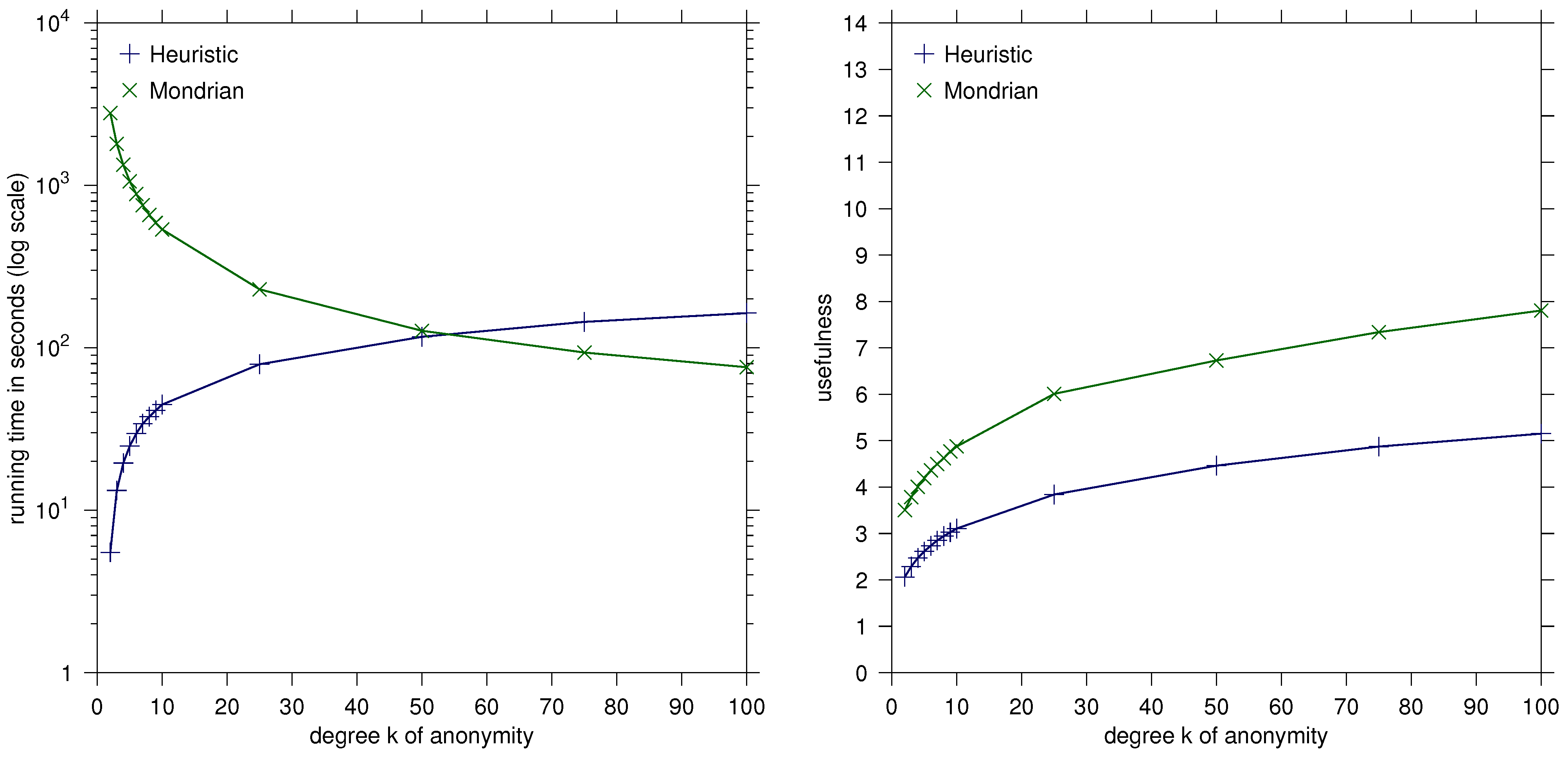
General Observations The running time behavior of the tested algorithms is somewhat unexpected. Whereas Mondrian gets faster with increasing k, our greedy heuristic gets faster with decreasing k. The reason why the greedy heuristic is faster for small values of k is that usually the cheap pattern vectors are used, and hence, the number of remaining input rows decreases soon. On the contrary, when k is large, the cheap pattern vectors cannot be used, and hence, the greedy heuristic tests many pattern vectors before it actually starts with removing rows from the input matrix. Thus, for larger values of k, the greedy heuristic comes closer to its worst-case running time of with .
Adult Our greedy heuristic could anonymize the Adult dataset in less than three minutes for all tested values of k. For and , Mondrian took more than half an hour to anonymize the dataset. However, in contrast to all other values of k, Mondrian was slightly faster for and . Except for with , all quality measures indicate that our heuristic produces the better solution.

| Greedy Heuristic | Mondrian | ||||||||||
|---|---|---|---|---|---|---|---|---|---|---|---|
| 2 | 2.062 | 5.502 | 14,589 | 2.232 | 16 | 2 | 3.505 | 2,789.400 | 11,136 | 2.709 | 61 |
| 3 | 2.290 | 13.226 | 9,208 | 3.536 | 18 | 3 | 3.782 | 1,803.510 | 7,306 | 4.128 | 61 |
| 4 | 2.470 | 19.538 | 6,670 | 4.882 | 25 | 4 | 4.007 | 1,337.860 | 5,432 | 5.553 | 61 |
| 5 | 2.615 | 24.867 | 5,199 | 6.263 | 31 | 5 | 4.191 | 1,061.960 | 4,325 | 6.974 | 61 |
| 6 | 2.738 | 29.663 | 4,315 | 7.546 | 42 | 6 | 4.362 | 885.939 | 3,597 | 8.385 | 61 |
| 7 | 2.851 | 34.126 | 3,669 | 8.875 | 53 | 7 | 4.498 | 754.652 | 3,053 | 9.879 | 61 |
| 8 | 2.942 | 37.629 | 3,193 | 10.198 | 53 | 8 | 4.622 | 659.184 | 2,663 | 11.326 | 61 |
| 9 | 3.026 | 41.216 | 2,832 | 11.498 | 52 | 9 | 4.766 | 588.347 | 2,368 | 12.737 | 69 |
| 10 | 3.106 | 44.779 | 2,559 | 12.724 | 56 | 10 | 4.875 | 535.872 | 2,145 | 14.062 | 69 |
| 25 | 3.840 | 79.281 | 1,046 | 31.129 | 161 | 25 | 6.009 | 229.248 | 850 | 35.485 | 90 |
| 50 | 4.462 | 117.008 | 537 | 60.635 | 317 | 50 | 6.729 | 127.392 | 430 | 70.144 | 135 |
| 75 | 4.873 | 144.536 | 354 | 91.980 | 317 | 75 | 7.339 | 93.621 | 287 | 105.094 | 242 |
| 100 | 5.151 | 163.582 | 274 | 118.836 | 317 | 100 | 7.805 | 76.005 | 209 | 144.316 | 242 |
The usefulness value of the Mondrian solutions is between and times the usefulness value of the heuristic for all tested k—this indicates the significantly better quality of the results of our heuristic. See Table 1 for details and Figure 1 for an illustration.
Adult-2 The solutions for Adult-2 behave similarly to those for Adult. Our greedy heuristic with a maximum running time of five seconds is significantly faster than Mondrian with a maximum running time of 20 min (at least 10 times faster for all tested k). However, the usefulness is quite similar for both algorithms. Mondrian beats the heuristic by less than 1% for ; the heuristic is slightly better for each other tested k. See Table 2 for details.
Nursery For the Nursery dataset, the heuristic is at least eight times faster than Mondrian. Concerning solution quality, this dataset is the most ambiguous one. Except for , Mondrian produces better solutions in terms of usefulness, whereas our heuristic performs better in terms of maximum and average output row type size. For the number of output row types, there is no clear winner. See Table 3 for details.
CMC For the CMC dataset, both algorithms were very fast in computing k-anonymous datasets for every tested k. Mondrian took at most 10 s, and our greedy heuristic took at most 1.2 s and was always faster than Mondrian. As for the solution quality, the heuristic can compete with Mondrian. The usefulness of the heuristic results is always slightly better. The Mondrian results have always at least 20% less output row types, and the average output row type size of the heuristic results is always smaller. Only for , and 8, the Mondrian results have a lower maximum size of the output row types. See Table 4 for details.
Figure 1.
Heuristic vs. Mondrian: Diagrams comparing running time and usefulness for the Adult dataset.
Figure 1.
Heuristic vs. Mondrian: Diagrams comparing running time and usefulness for the Adult dataset.

| Greedy Heuristic | Mondrian | ||||||||||
|---|---|---|---|---|---|---|---|---|---|---|---|
| 2 | 1.760 | 1.040 | 12,022 | 2.708 | 45 | 2 | 1.885 | 1,278.380 | 7,971 | 3.784 | 113 |
| 3 | 1.872 | 1.181 | 7,971 | 4.085 | 45 | 3 | 1.992 | 887.699 | 5,543 | 5.441 | 113 |
| 4 | 1.962 | 1.329 | 5,890 | 5.528 | 45 | 4 | 2.074 | 693.385 | 4,319 | 6.984 | 113 |
| 5 | 2.037 | 1.504 | 4,609 | 7.065 | 45 | 5 | 2.142 | 565.370 | 3,525 | 8.557 | 113 |
| 6 | 2.099 | 1.629 | 3,836 | 8.488 | 45 | 6 | 2.201 | 484.160 | 3,020 | 9.987 | 113 |
| 7 | 2.161 | 1.707 | 3,266 | 9.970 | 52 | 7 | 2.257 | 417.950 | 2,596 | 11.619 | 113 |
| 8 | 2.212 | 1.796 | 2,837 | 11.477 | 63 | 8 | 2.291 | 372.469 | 2,308 | 13.068 | 113 |
| 9 | 2.260 | 1.936 | 2,518 | 12.931 | 63 | 9 | 2.325 | 338.958 | 2,095 | 14.397 | 113 |
| 10 | 2.302 | 2.025 | 2,273 | 14.325 | 66 | 10 | 2.366 | 308.058 | 1,890 | 15.959 | 113 |
| 25 | 2.722 | 2.926 | 914 | 35.625 | 164 | 25 | 2.724 | 139.030 | 801 | 37.655 | 113 |
| 50 | 3.094 | 3.874 | 460 | 70.785 | 349 | 50 | 3.070 | 79.263 | 414 | 72.855 | 145 |
| 75 | 3.312 | 4.426 | 310 | 105.035 | 552 | 75 | 3.385 | 59.847 | 277 | 108.888 | 200 |
| 100 | 3.434 | 4.928 | 245 | 132.902 | 552 | 100 | 3.573 | 49.573 | 210 | 143.629 | 279 |
| Greedy Heuristic | Mondrian | ||||||||||
|---|---|---|---|---|---|---|---|---|---|---|---|
| 2 | 3.200 | 0.834 | 4,320 | 3.000 | 3 | 2 | 2.776 | 484.572 | 6,468 | 2.004 | 3 |
| 3 | 3.200 | 0.285 | 4,320 | 3.000 | 3 | 3 | 3.057 | 233.710 | 3,294 | 3.934 | 4 |
| 4 | 3.283 | 0.344 | 3,240 | 4.000 | 4 | 4 | 3.072 | 221.731 | 3,186 | 4.068 | 6 |
| 5 | 3.333 | 0.328 | 2,592 | 5.000 | 5 | 5 | 3.338 | 122.665 | 1,722 | 7.526 | 8 |
| 6 | 3.867 | 0.320 | 1,440 | 9.000 | 9 | 6 | 3.338 | 122.713 | 1,722 | 7.526 | 8 |
| 7 | 3.867 | 0.335 | 1,440 | 9.000 | 9 | 7 | 3.396 | 104.568 | 1,518 | 8.538 | 12 |
| 8 | 3.867 | 0.391 | 1,440 | 9.000 | 9 | 8 | 3.396 | 104.638 | 1,518 | 8.538 | 12 |
| 9 | 3.867 | 0.319 | 1,440 | 9.000 | 9 | 9 | 3.607 | 67.630 | 922 | 14.056 | 16 |
| 10 | 3.950 | 0.432 | 1,080 | 12.000 | 12 | 10 | 3.607 | 68.079 | 922 | 14.056 | 16 |
| 25 | 4.533 | 0.846 | 480 | 27.000 | 27 | 25 | 4.091 | 28.229 | 334 | 38.802 | 48 |
| 50 | 4.750 | 1.179 | 216 | 60.000 | 60 | 50 | 4.493 | 18.330 | 176 | 73.636 | 96 |
| 75 | 4.833 | 1.259 | 162 | 80.000 | 80 | 75 | 4.720 | 13.638 | 116 | 111.724 | 144 |
| 100 | 5.283 | 1.608 | 120 | 108.000 | 108 | 100 | 4.861 | 13.179 | 100 | 129.600 | 144 |
| Greedy Heuristic | Mondrian | ||||||||||
|---|---|---|---|---|---|---|---|---|---|---|---|
| 2 | 3.274 | 0.068 | 718 | 2.052 | 4 | 2 | 3.469 | 9.134 | 599 | 2.459 | 7 |
| 3 | 3.508 | 0.111 | 461 | 3.195 | 7 | 3 | 3.814 | 6.375 | 391 | 3.767 | 8 |
| 4 | 3.735 | 0.152 | 334 | 4.410 | 9 | 4 | 4.139 | 4.848 | 273 | 5.396 | 10 |
| 5 | 3.934 | 0.178 | 258 | 5.709 | 15 | 5 | 4.331 | 4.205 | 223 | 6.605 | 11 |
| 6 | 4.115 | 0.212 | 216 | 6.819 | 17 | 6 | 4.538 | 3.729 | 184 | 8.005 | 13 |
| 7 | 4.219 | 0.244 | 183 | 8.049 | 17 | 7 | 4.724 | 3.328 | 155 | 9.503 | 16 |
| 8 | 4.410 | 0.251 | 158 | 9.323 | 18 | 8 | 4.913 | 3.085 | 135 | 10.911 | 17 |
| 9 | 4.500 | 0.288 | 139 | 10.597 | 18 | 9 | 5.023 | 2.914 | 122 | 12.074 | 21 |
| 10 | 4.545 | 0.282 | 127 | 11.598 | 18 | 10 | 5.178 | 2.717 | 108 | 13.639 | 21 |
| 25 | 5.641 | 0.447 | 48 | 30.688 | 53 | 25 | 6.434 | 1.862 | 43 | 34.256 | 57 |
| 50 | 6.319 | 0.559 | 27 | 54.556 | 77 | 50 | 7.272 | 1.556 | 22 | 66.955 | 95 |
| 75 | 6.926 | 0.685 | 17 | 86.647 | 148 | 75 | 7.836 | 1.404 | 13 | 113.308 | 148 |
| 100 | 7.271 | 0.752 | 13 | 113.308 | 167 | 100 | 7.981 | 1.368 | 10 | 147.300 | 204 |
| Greedy Heuristic | Mondrian | ||||||||||
|---|---|---|---|---|---|---|---|---|---|---|---|
| 2 | 1.403 | 13.018 | 63,140 | 5.139 | 2,448 | 2 | 1.476 | 3,504.560 | 15,984 | 2.409 | 9 |
| 3 | 1.415 | 13.599 | 41,408 | 7.836 | 2,448 | 3 | 1.577 | 2,196.720 | 10,233 | 3.763 | 11 |
| 4 | 1.429 | 14.679 | 31,652 | 10.252 | 2,448 | 4 | 1.654 | 1,600.540 | 7,458 | 5.163 | 12 |
| 5 | 1.442 | 14.870 | 25,852 | 12.552 | 2,448 | 5 | 1.714 | 1,252.050 | 5,887 | 6.540 | 13 |
| 6 | 1.456 | 15.318 | 22,150 | 14.650 | 2,448 | 6 | 1.766 | 1,040.750 | 4,856 | 7.929 | 15 |
| 7 | 1.469 | 15.434 | 19,399 | 16.727 | 2,448 | 7 | 1.803 | 894.510 | 4,139 | 9.302 | 17 |
| 8 | 1.482 | 16.071 | 17,276 | 18.783 | 2,448 | 8 | 1.834 | 783.056 | 3,618 | 10.642 | 19 |
| 9 | 1.495 | 16.198 | 15,651 | 20.733 | 2,448 | 9 | 1.863 | 694.625 | 3,191 | 12.066 | 22 |
| 10 | 1.508 | 16.631 | 14,248 | 22.774 | 2,448 | 10 | 1.888 | 622.441 | 2,840 | 13.557 | 27 |
| 25 | 1.646 | 20.154 | 6,167 | 52.617 | 2,448 | 25 | 2.119 | 272.739 | 1,120 | 34.378 | 57 |
| 50 | 1.773 | 23.383 | 2,988 | 108.597 | 2,448 | 50 | 2.354 | 158.413 | 563 | 68.389 | 103 |
| 75 | 1.861 | 25.736 | 1,917 | 169.269 | 2,448 | 75 | 2.516 | 116.970 | 356 | 108.154 | 154 |
| 100 | 1.929 | 27.600 | 1,393 | 232.942 | 2,838 | 100 | 2.595 | 103.402 | 279 | 138.004 | 201 |
Canada Again, our heuristic outperforms Mondrian in terms of efficiency (at least three times faster). However, for this dataset, the quality measures are contradictory. Whereas the usefulness of the heuristic results is always slightly better and the number of output row types of the heuristic results is at least four times the number of output row types of Mondrian results, the measures concerning the size of the output row types are significantly better for Mondrian. The reason seems that our heuristic always produces one block of at least 2,448 identical rows. See Table 5 for details.
Conclusions for Classical k-Anonymity We showed that our greedy heuristic is very efficient, even for real-world datasets with more than 100,000 records and . Especially for smaller degrees of anonymity , Mondrian is at least ten times slower. Altogether, our heuristic outperforms Mondrian for all datasets, except Nursery, in terms of the quality of the solution. There is no clear winner for the Nursery dataset. Hence, we demonstrated that even when neglecting the feature of pattern-guidedness and simply specifying all possible pattern vectors, our heuristic already produces useful solutions that can at least compete with Mondrian’s solutions.
3.6. Heuristic vs. Exact Solution
In Section 3.5, we showed that our greedy heuristic is very efficient and produces good solutions, even if it is (mis)used to solve the classical k-Anonymity problem.
By design, the heuristic always produces solutions where every output row can be matched to some of the specified pattern vectors. However, the number of suppressions performed may be far from being optimal. Hence, by comparing with the exact solutions of the ILP implementation, we try to answer the question of how far the produced solutions are away from the optimum. We evaluate our experiments using the following criteria:
- Number s of suppressions;
- Usefulness value u;
- Running time r in seconds;
- Number of output row types;
- Average size of the output row types; and
- Maximum size of the output row types.
Nursery Our ILP implementation was able to k-anonymize the Nursery dataset for , 25, 50, 75, 100} within two minutes for each input, that is, we could solve k-Anonymity with a minimum number of suppressions. In contrast, the ILP formulation could not k-anonymize the other datasets within 30 min for many values of k.
Surprisingly, the results computed by the heuristic were optimal (in terms of the number of suppressed entries) for all tested k, and many results are better in terms of the other quality measures. The reason seems to be that the ILP implementation tends to find, for a fixed number of suppressions, solutions with a high degree of anonymity. For example, the result of the ILP for is already 15-anonymous, whereas the result of the heuristic is 9-anonymous, yielding more and smaller output row types. Summarizing, the heuristic is at least 25 times faster than the ILP implementation and also produces solutions with a minimum number of suppressions, which have a better quality concerning , and values. See Table 6 for details.
CMC Consider the scenario where the user is interested in a k-anonymized version of the CMC dataset, where each row has at most two suppressed entries. To fulfill these constraints, we specified all possible pattern vectors with at most two ☆-symbols (plus the all-☆-vector to remove outliers) and applied our greedy heuristic and the ILP implementation for , 25, 50, 75, 100}.
As expected, the heuristic works much faster than the ILP implementation (at least by a factor of ten). The solution quality depends on the anonymity degree k. The results of the heuristic get closer to the optimum with increasing k. Whereas for , the number of suppressions in the heuristic solution is times the optimum, for , the heuristic produces results with a minimum number of suppressions. Most other quality measures behave similarly, but the differences are less strong. The usefulness values of the heuristic results are at most as good as those of the ILP results for and . See Table 7 for details.
Adult-2 Consider a user who is interested in the Adult-2 dataset. Her main goal is to analyze correlations between the income of the individuals and the other attributes (to detect discrimination). To get useful data, she specifies four constraints for an anonymized record.
- Each record should contain at most two suppressed entries.
- The attributes “education” and “salary class” should not be suppressed, because she assumes a strong relation between them.
- One of the attributes, “work class” or “occupation”, alone is useless for her, so either both should be suppressed or none of them.
| Greedy Heuristic | ILP implementation | ||||||||||||
|---|---|---|---|---|---|---|---|---|---|---|---|---|---|
| 2 | 12,690 | 3.20 | 0.834 | 4320 | 3.0 | 3 | 2 | 12,960 | 3.20 | 62.859 | 4,320 | 3.0 | 3 |
| 3 | 12,690 | 3.20 | 0.285 | 4320 | 3.0 | 3 | 3 | 12,960 | 3.20 | 62.627 | 4,320 | 3.0 | 3 |
| 4 | 12,690 | 3.28 | 0.344 | 3240 | 4.0 | 4 | 4 | 12,960 | 3.33 | 61.097 | 2,592 | 5.0 | 5 |
| 5 | 12,690 | 3.33 | 0.328 | 2592 | 5.0 | 5 | 5 | 12,960 | 3.33 | 60.543 | 2,592 | 5.0 | 5 |
| 6 | 25,920 | 3.87 | 0.320 | 1440 | 9.0 | 9 | 6 | 25,920 | 4.0 | 60.812 | 864 | 15.0 | 15 |
| 7 | 25,920 | 3.87 | 0.335 | 1440 | 9.0 | 9 | 7 | 25,920 | 4.0 | 47.496 | 864 | 15.0 | 15 |
| 8 | 25,920 | 3.87 | 0.391 | 1440 | 9.0 | 9 | 8 | 25,920 | 4.0 | 59.188 | 864 | 15.0 | 15 |
| 9 | 25,920 | 3.87 | 0.319 | 1440 | 9.0 | 9 | 9 | 25,920 | 4.0 | 59.717 | 864 | 15.0 | 15 |
| 10 | 25,920 | 3.95 | 0.432 | 1080 | 12.0 | 12 | 10 | 25,920 | 4.0 | 59.334 | 864 | 15.0 | 15 |
| 25 | 38,880 | 4.53 | 0.846 | 480 | 27.0 | 27 | 25 | 38,880 | 4.75 | 56.221 | 216 | 60.0 | 60 |
| 50 | 38,880 | 4.75 | 1.179 | 216 | 60.0 | 60 | 50 | 38,880 | 4.75 | 49.699 | 216 | 60.0 | 60 |
| 75 | 38,880 | 4.83 | 1.259 | 162 | 80.0 | 80 | 75 | 38,880 | 4.83 | 45.728 | 162 | 80.0 | 80 |
| 100 | 51,840 | 5.28 | 1.608 | 120 | 108.0 | 108 | 100 | 51,840 | 5.5 | 44.085 | 54 | 240.0 | 240 |
Table 7.
Heuristic vs. ILP: Results for the CMC dataset specifying all pattern vectors with costs of at most two.
| Greedy Heuristic | ILP implementation | ||||||||||||
|---|---|---|---|---|---|---|---|---|---|---|---|---|---|
| 2 | 4,112 | 3.18 | 0.057 | 533 | 2.764 | 249 | 2 | 2,932 | 3.22 | 2.205 | 653 | 2.256 | 100 |
| 3 | 6,564 | 3.42 | 0.054 | 264 | 5.580 | 501 | 3 | 5,216 | 3.46 | 3.668 | 349 | 4.221 | 320 |
| 4 | 8,252 | 3.57 | 0.066 | 153 | 9.627 | 696 | 4 | 7,024 | 3.60 | 2.240 | 208 | 7.082 | 528 |
| 5 | 8,952 | 3.69 | 0.069 | 109 | 13.514 | 771 | 5 | 8,065 | 3.73 | 3.939 | 146 | 10.089 | 646 |
| 6 | 9,821 | 3.76 | 0.072 | 78 | 18.885 | 874 | 6 | 9,012 | 3.80 | 1.655 | 103 | 14.301 | 765 |
| 7 | 10,339 | 3.84 | 0.084 | 61 | 24.148 | 935 | 7 | 9,751 | 3.84 | 1.479 | 76 | 19.382 | 856 |
| 8 | 10,878 | 3.95 | 0.073 | 47 | 31.340 | 998 | 8 | 10,254 | 3.91 | 1.454 | 60 | 24.550 | 918 |
| 9 | 11,486 | 4.06 | 0.085 | 32 | 46.031 | 1,074 | 9 | 11,051 | 4.00 | 1.269 | 44 | 33.477 | 1016 |
| 10 | 11,678 | 4.08 | 0.081 | 28 | 52.607 | 1,098 | 10 | 11,462 | 4.05 | 1.364 | 35 | 42.086 | 1066 |
| 25 | 13,722 | 5.69 | 0.097 | 4 | 368.25 | 1,347 | 25 | 13,722 | 5.37 | 1.106 | 5 | 294.60 | 1347 |
| 50 | 14,314 | 7.12 | 0.103 | 2 | 736.50 | 1,421 | 50 | 14,314 | 7.12 | 1.174 | 2 | 736.50 | 1421 |
| 75 | 14,730 | 10.0 | 0.108 | 1 | 1,473.0 | 1,473 | 75 | 14,730 | 10.0 | 1.169 | 1 | 1,473.0 | 1473 |
| 100 | 14,730 | 10.0 | 0.097 | 1 | 1,473.0 | 1,473 | 100 | 14,730 | 10.0 | 1.146 | 1 | 1,473.0 | 1473 |
| Greedy Heuristic | ILP implementation | ||||||||||||
|---|---|---|---|---|---|---|---|---|---|---|---|---|---|
| 2 | 38,312 | 1.73 | 0.61 | 9,214 | 3.53 | 2,356 | 2 | 29,056 | 1.75 | 19.91 | 9,765 | 3.33 | 893 |
| 3 | 55,749 | 1.81 | 0.57 | 5,313 | 6.13 | 3,896 | 3 | 43,887 | 1.84 | 41.36 | 6,315 | 5.16 | 1,831 |
| 4 | 67,618 | 1.87 | 0.55 | 3,676 | 8.86 | 5,077 | 4 | 54,162 | 1.91 | 53.13 | 4,754 | 6.85 | 2,592 |
| 5 | 76,363 | 1.91 | 0.60 | 2,777 | 11.7 | 5,967 | 5 | 61,701 | 1.96 | 163.9 | 4,034 | 8.07 | 3,183 |
| 6 | 83,598 | 1.95 | 0.60 | 2,214 | 14.7 | 6,736 | 6 | 68,278 | 2.01 | 183.1 | 3,386 | 9.62 | 3,737 |
| 7 | 89,501 | 1.99 | 0.65 | 1,849 | 17.6 | 7,346 | 7 | 74,160 | 2.06 | 322.7 | 2,833 | 11.5 | 4,275 |
| 8 | 94,086 | 2.02 | 0.62 | 1,581 | 20.6 | 7,801 | 8 | 79,109 | 2.08 | 110.3 | 2,509 | 13.0 | 4,846 |
| 9 | 98,999 | 2.04 | 0.63 | 1,360 | 23.9 | 8,333 | 9 | 84,065 | 2.11 | 68.58 | 2,046 | 15.9 | 5,560 |
| 10 | 103,624 | 2.07 | 0.68 | 1,194 | 27.3 | 8,863 | 10 | 88,026 | 2.15 | 52.39 | 1,762 | 18.5 | 5,997 |
| 25 | 141,697 | 2.31 | 0.75 | 395 | 82.4 | 13,237 | 25 | 125,233 | 2.43 | 18.43 | 684 | 47.6 | 10,046 |
| 50 | 173,947 | 2.53 | 0.85 | 164 | 198 | 17,110 | 50 | 161,083 | 2.62 | 7.067 | 288 | 113 | 14,636 |
| 75 | 196,218 | 2.57 | 0.93 | 97 | 336 | 20,040 | 75 | 185,870 | 2.69 | 6.179 | 153 | 213 | 18,063 |
| 100 | 207,417 | 2.57 | 0.93 | 73 | 446 | 21,465 | 100 | 197,421 | 2.74 | 6.552 | 102 | 319 | 19,648 |
- 4.
- Since she assumes discrimination because of age, sex, and race, at most one of these attributes should be suppressed.
The ILP implementation took up to six minutes to compute one single instance, whereas the greedy heuristic needs always less than one second. Moreover, the solution quality of the heuristic results is surprisingly good. The number of suppressed entries is at most times the optimum. The ILP is slightly better concerning the measures and . Only the maximum size of the output row types of the heuristic results is sometimes more than twice the maximum size of output row types of the ILP results for some k. Surprisingly, the usefulness values are always slightly better for the heuristic results. See Table 8 for details.
4. Conclusions
In three scenarios with real-world datasets, we showed that our greedy heuristic performs well in terms of solution quality compared with the optimal solution produced by the ILP implementation. The results of the heuristic are relatively close to the optimum, and in fact, for many cases, they were optimal, although our heuristic is much more efficient than the exact algorithm (the ILP was, on average, more than 1000 times slower). The heuristic results tend to get closer to the optimal number of suppressions with increasing degree k of anonymity.
5. Outlook
We introduced a promising approach to combinatorial data anonymization by enhancing the basic k-Anonymity problem with user-provided “suppression patterns.” It seems feasible to extend our model with weights on the attributes, thus making user influence on the anonymization process even more specific. A natural next step is to extend our model by replacing k-Anonymity by more refined data privacy concepts, such as domain generalization hierarchies [40], p-sensitivity [41], ℓ-diversity [23] and t-closeness [38].
On the theoretical side, we did no extensive analysis of the polynomial-time approximability of Pattern-Guided k-Anonymity. Are there provably good approximation algorithms for Pattern-Guided k-Anonymity? Concerning exact solutions, are there further polynomial-time solvable special cases beyond Pattern-Guided 2-Anonymity?
On the experimental side, several issues remain to be attacked. For instance, we used integer linear programming in a fairly straightforward way almost without any tuning tricks (e.g., using the heuristic solution or “standard heuristics” for speeding up integer linear program solving). It also remains to perform tests comparing our heuristic algorithm against methods other than Mondrian (unfortunately, for the others, no source code seems to be freely available).
Acknowledgments
We thank our students, Thomas Köhler and Kolja Stahl, for their great support in doing implementations and experiments. We are grateful to anonymous reviewers of Algorithms for constructive and extremely fast feedback (including the spotting of a bug in the proof of Theorem 4) that helped to improve our presentation. Robert Bredereck was supported by the DFG, research project PAWS, NI 369/10.
Conflicts of Interest
The authors declare no conflicts of interest.
References
- Fung, B.C.M.; Wang, K.; Chen, R.; Yu, P.S. Privacy-preserving data publishing: A survey of recent developments. ACM Comput. Surv. 2010, 42, 14:1–14:53. [Google Scholar] [CrossRef]
- Navarro-Arribas, G.; Torra, V.; Erola, A.; Castellà-Roca, J. User k-anonymity for privacy preserving data mining of query logs. Inf. Process. Manag. 2012, 48, 476–487. [Google Scholar] [CrossRef]
- Dwork, C. A firm foundation for private data analysis. Commun. ACM 2011, 54, 86–95. [Google Scholar] [CrossRef]
- Bonizzoni, P.; Della Vedova, G.; Dondi, R. Anonymizing binary and small tables is hard to approximate. J. Comb. Optim. 2011, 22, 97–119. [Google Scholar] [CrossRef]
- Bonizzoni, P.; Della Vedova, G.; Dondi, R.; Pirola, Y. Parameterized complexity of k-anonymity: Hardness and tractability. J. Comb. Optim. 2013, 26, 19–43. [Google Scholar] [CrossRef]
- Chakaravarthy, V.T.; Pandit, V.; Sabharwal, Y. On the complexity of the k-anonymization problem. 2010; arXiv:1004.4729. [Google Scholar]
- Blocki, J.; Williams, R. Resolving the Complexity of Some Data Privacy Problems. In Proceedings of the 37th International Colloquium on Automata, Languages and Programming (ICALP ’10), Bordeaux, France, 6–10 July 2010; Springer: Berlin/Heidelberg, Germany, 2010; Volume 6199, LNCS. pp. 393–404. [Google Scholar]
- Meyerson, A.; Williams, R. On the Complexity of Optimal k-Anonymity. In Proceedings of the 23rd ACM SIGMOD-SIGACT-SIGART Symposium on Principles of Database Systems (PODS ’04), Paris, France, 14–16 June 2004; ACM: New York, NY, USA, 2004; pp. 223–228. [Google Scholar]
- Campan, A.; Truta, T.M. Data and Structural k-Anonymity in Social Networks. In Proceedings of the 2nd ACM SIGKDD International Workshop on Privacy, Security, and Trust in KDD (PinKDD ’08), Las Vegas, NV, USA, 24 August 2008; Springer: Berlin/Heidelberg, Germany, 2009; Volume 5456, LNCS. pp. 33–54. [Google Scholar]
- Gkoulalas-Divanis, A.; Kalnis, P.; Verykios, V.S. Providing k-Anonymity in location based services. ACM SIGKDD Explor. Newslett. 2010, 12, 3–10. [Google Scholar] [CrossRef]
- Loukides, G.; Shao, J. Capturing Data Usefulness and Privacy Protection in k-Anonymisation. In Proceedings of the 2007 ACM Symposium on Applied Computing, Seoul, Korea, 11–15 March 2007; ACM: New York, NY, USA, 2007; pp. 370–374. [Google Scholar]
- Rastogi, V.; Suciu, D.; Hong, S. The Boundary between Privacy and Utility in Data Publishing. In Proceedings of the 33rd International Conference on Very Large Data Bases, VLDB Endowment, Vienna, Austria, 23–27 September 2007; pp. 531–542.
- Bredereck, R.; Nichterlein, A.; Niedermeier, R.; Philip, G. Pattern-Guided Data Anonymization and Clustering. In Proceedings of the 36th International Symposium on Mathematical Foundations of Computer Science (MFCS ’11), Warsaw, Poland, 22–26 August 2011; Springer: Berlin/Heidelberg, Germany, 2011; Volume 6907, LNCS. pp. 182–193. [Google Scholar]
- Bredereck, R.; Köhler, T.; Nichterlein, A.; Niedermeier, R.; Philip, G. Using patterns to form homogeneous teams. Algorithmica 2013. [Google Scholar] [CrossRef]
- Samarati, P. Protecting respondents identities in microdata release. IEEE Trans. Knowl. Data Eng. 2001, 13, 1010–1027. [Google Scholar] [CrossRef]
- Samarati, P.; Sweeney, L. Generalizing Data to Provide Anonymity When Disclosing Information. In Proceedings of the ACM SIGACT-SIGMOD-SIGART Symposium on Principles of Database Systems (PODS ’98), Seattle, WA, USA, 1–3 June 1998; ACM: New York, NY, USA, 1998; pp. 188–188. [Google Scholar]
- Sweeney, L. k-anonymity: A model for protecting privacy. Int. J. Uncertain. Fuzziness Knowl.-Based Syst. 2002, 10, 557–570. [Google Scholar] [CrossRef]
- Downey, R.G.; Fellows, M.R. Parameterized Complexity; Springer: Berlin/Heidelberg, Germany, 1999. [Google Scholar]
- Flum, J.; Grohe, M. Parameterized Complexity Theory; Springer: Berlin/Heidelberg, Germany, 2006. [Google Scholar]
- Niedermeier, R. Invitation to Fixed-Parameter Algorithms; Oxford University Press: Oxford, UK, 2006. [Google Scholar]
- LeFevre, K.; DeWitt, D.; Ramakrishnan, R. Mondrian Multidimensional k-anonymity. In Proceedings of the IEEE 22nd International Conference on Data Engineering (ICDE ’06), Atlanta, GA, USA, 3–7 April 2006; IEEE Computer Society: Washington, DC, USA, 2006; pp. 25–25. [Google Scholar]
- Frank, A.; Asuncion, A. UCI Machine Learning Repository, University of California, Irvine, School of Information and Computer Sciences. 2010. http://archive.ics.uci.edu/ml.
- Machanavajjhala, A.; Kifer, D.; Gehrke, J.; Venkitasubramaniam, M. ℓ-diversity: Privacy beyond k-anonymity. ACM Trans. Knowl. Discov. Data 2007, 1. [Google Scholar] [CrossRef]
- Evans, P.A.; Wareham, T.; Chaytor, R. Fixed-parameter tractability of anonymizing data by suppressing entries. J. Comb. Optim. 2009, 18, 362–375. [Google Scholar] [CrossRef]
- Karp, R.M. Reducibility Among Combinatorial Problems. In Complexity of Computer Computations; Miller, R.E., Thatcher, J.W., Eds.; Plenum Press: New York, NY, USA, 1972; pp. 85–103. [Google Scholar]
- Anshelevich, E.; Karagiozova, A. Terminal backup, 3D matching, and covering cubic graphs. SIAM J. Comput. 2011, 40, 678–708. [Google Scholar] [CrossRef]
- Bredereck, R.; Nichterlein, A.; Niedermeier, R.; Philip, G. The effect of homogeneity on the computational complexity of combinatorial data anonymization. Data Min. Knowl. Discov. 2012. [Google Scholar] [CrossRef]
- Fredkin, E. Trie memory. Commun. ACM 1960, 3, 490–499. [Google Scholar] [CrossRef]
- Lenstra, H.W. Integer programming with a fixed number of variables. Math. Oper. Res. 1983, 8, 538–548. [Google Scholar] [CrossRef]
- Adult dataset. Available online: ftp://ftp.ics.uci.edu/pub/machine-learning-databases/adult/ (accessed on 16 October 2013).
- Nursery dataset. Available online: ftp://ftp.ics.uci.edu/pub/machine-learning-databases/nursery/ (accessed on 16 October 2013).
- Olave, M.; Rajkovic, V.; Bohanec, M. An application for admission in public school systems. Expert Syst. Public Adm. 1989, 145, 145–160. [Google Scholar]
- CMC dataset. Available online: ftp://ftp.ics.uci.edu/pub/machine-learning-databases/cmc/ (accessed on 16 October 2013).
- Canada dataset. Available online: http://www.hc-sc.gc.ca/dhp-mps/medeff/databasdon/index-eng.php (accessed on 16 October 2013).
- Canada attribute names. Available online: http://www.hc-sc.gc.ca/dhp-mps/medeff/databasdon/structure-eng.php#a1 (accessed on 16 October 2013).
- Mainland, G.; Leshchinskiy, R.; Peyton Jones, S. Exploiting Vector Instructions with Generalized Stream Fusion. In Proceedings of the 18th ACM SIGPLAN International Conference on Functional Programming (ICFP ’13), Boston, MA, USA, 25–27 September 2013; ACM: New York, NY, USA, 2013; pp. 37–48. [Google Scholar]
- Pattern-Guided k-Anonymity heuristic. Available online: http://akt.tu-berlin.de/menue/software/ (accessed on 16 October 2013).
- Li, N.; Li, T.; Venkatasubramanian, S. t-Closeness: Privacy Beyond k-Anonymity and l-Diversity. In Proceedings of the IEEE 23rd International Conference on Data Engineering (ICDE ’07), Istanbul, Turkey, 15–20 April 2007; pp. 106–115.
- Mondrian implementation. Available online: http://cs.utdallas.edu/dspl/cgi-bin/toolbox/ index.php?go=home (accessed on 16 October 2013).
- Sweeney, L. Achieving k-anonymity privacy protection using generalization and suppression. Int. J. Uncertain. Fuzziness Knowl.-Based Syst. 2002, 10, 571–588. [Google Scholar] [CrossRef]
- Truta, T.M.; Vinay, B. Privacy Protection: p-Sensitive k-Anonymity Property. In Proceedings of the 22nd International Conference on Data Engineering Workshops (ICDE ’06), Atlanta, GA, USA, 3–7 April 2006; IEEE Computer Society: Washington, DC, USA, 2006; p. 94. [Google Scholar]
© 2013 by the authors; licensee MDPI, Basel, Switzerland. This article is an open access article distributed under the terms and conditions of the Creative Commons Attribution license (http://creativecommons.org/licenses/by/3.0/).
Share and Cite
MDPI and ACS Style
Bredereck, R.; Nichterlein, A.; Niedermeier, R. Pattern-Guided k-Anonymity. Algorithms 2013, 6, 678-701. https://0-doi-org.brum.beds.ac.uk/10.3390/a6040678
AMA Style
Bredereck R, Nichterlein A, Niedermeier R. Pattern-Guided k-Anonymity. Algorithms. 2013; 6(4):678-701. https://0-doi-org.brum.beds.ac.uk/10.3390/a6040678
Chicago/Turabian StyleBredereck, Robert, André Nichterlein, and Rolf Niedermeier. 2013. "Pattern-Guided k-Anonymity" Algorithms 6, no. 4: 678-701. https://0-doi-org.brum.beds.ac.uk/10.3390/a6040678