1. Introduction
Inspired by many deadlock detection applications, the Feedback Vertex Set Problem (FVSP) is known to be NP-complete and plays an important role in the study of deadlock recovery [
1,
2]. For example, the wait-for graph is a directed graph used for deadlock detection in operating systems and relational database systems of an operating system. and each directed cycle corresponds to a deadlock situation in the wait-for graph. In order to resolve all deadlocks, some blocked processes need to be aborted. A minimum feedback vertex set in this graph corresponds to a minimum number of processes that one needs to abort. Therefore solving the FVSP with more efficiency and better performance can contribute to an improved deadlock recovery.
To describe the FVSP, the following concepts are predefined. Assuming is a graph, then the set of vertices is denoted by , and the set of edges of G is denoted by . For , the subgraph induced by S is denoted by . The set of vertices adjacent to a vertex, , will be denoted by and called the of the vertex, i. Let G be a graph. A feedback vertex set, S, in G is a set of vertices in G, whose removal results in a graph without cycle (or equivalently, every cycle in G contains at least one vertex in S).
The FVSP can be considered in both directed and undirected graphs.Let G be an undirected graph. A Feedback Vertex Set Problem (FVSP), S, in G is a set of vertices in G, whose removal results in a graph without cycle (or equivalently, every cycle in G contains at least one vertex in S). Let G be a directed graph. A feedback vertex set (FVS), S, in G is a set of vertices in G, whose removal results in a graph without directed cycle (or equivalently, every directed cycle in G contains at least one vertex in S).
Inspired by real world applications, several variants were proposed over the years. Some of them are summarized by the following definitions.
- (a)
FVSP: Given a graph, G, the feedback vertex set problem is to find an FVS with the minimum cardinality.
- (b)
The Parameterized Feedback Vertex Set Problem (DFVSP): Given a graph, G, and a parameter, k, the Parameterized Feedback Vertex Set Problem is to either find an FVS of at most k vertices for G or report that no such set exists.
- (c)
The Vertex Weighted Feedback Vertex Set Problem (VWFVSP): Given a vertex weighted graph, G, the Vertex Weighted Feedback Vertex Set Problem is to find an FVS with the minimum weight.
The Parameterized Feedback Vertex Set Problem is the decision version of the feedback vertex set problem. The FVSP and DFVSP were classic NP-complete problems that appeared in the first list of NP-complete problems in Karp’s seminal paper [
3]. When the edges or arcs instead of vertices are considered, it becomes the corresponding edge or arc version. For example, the parameterized feedback arc set problem is to find out whether there is a minimum of
k arcs in a given graph, whose removal makes the graph acyclic.
Let G be a graph. It is said that a vertex set, S, is an acyclic vertex set if is acyclic. An acyclic vertex set, S, is maximal if is not acyclic for any . Note that if is acyclic, then is a feedback vertex set.
Without loss of generality, only the feedback vertex set problem for an undirected graph is considered in this paper, and the aim is to search for the largest subset, , such that is acyclic.
The rest of this paper is organized as follows:
Section 2 presents the related work of local search heuristics. Then,
Section 3 and
Section 4 propose the
k-opt local search (KLS)-based local search algorithm and the KLS with a randomized scheme algorithm in detail.
Section 5 conducts the experiments of both the proposed algorithms and the compared metaheuristics with the results for the performance and efficiency evaluation. Finally,
Section 6 discusses the contributions of this paper and draws a conclusion.
2. Related Work
As a local improved technology, the local search is a practical tool and a common technique looking for the near-optimal solutions for combinatorial optimization problems [
4]. In order to obtain high-quality solutions, it was applied to many metaheuristic algorithms, such as simulating annealing, genetic algorithm, memetic algorithm and swarm intelligent algorithms, in many cases.
The local search is a common tool looking for near-optimal solutions in reasonable time for combinatorial optimization problems. Usually, the current solution is iteratively replaced by an improved solution from its neighborhood, until no better solution can be obtained. Then, the current solution is called locally optimal.
The basic local search starts with a feasible solution,
x, and repeatedly replaces
x with an improved one,
, which is selected from the neighborhood of
x. If no better neighbor solutions can be found in its neighborhood, the local search immediately stops and returns as the final best solution found during the search [
4].
Since the basic local search is usually unable to obtain a good-quality solution and often far from the optimal solution, various improved local searches were proposed, e.g., tabu search [
5,
6,
7], variable depth search [
8,
9], variable neighborhood search [
10,
11,
12], reactive local search [
13,
14,
15,
16],
k-opt local search (KLS) [
4,
17], iterated local search [
18], iterated
k-opt local search [
17] and phased local search [
19].
In many cases, the local search can be applied into heuristic algorithms, such as simulated annealing, ant colony and particle swarm optimizations. However, normally, it is hard to obtain the best solution, or even an approximate solution with high quality, for a certain combinatorial optimization problem. Therefore, various local search methods, such as phased local search [
19] and variable depth local search, were proposed. The variable depth local search was initially used to solve the Graph Partitioning Problem (GPP) [
9] and the Traveling Salesman Problem (TSP) [
8]. Then, it was applied to other heuristic algorithms [
20,
21,
22,
23]. In [
4], it was applied to solve the maximum clique problem and successfully obtained good solutions.
Different from the previous studies, the proposed local search algorithms are based on KLS and are combined with a depth variable search, which can improve the performance and efficiency.
3. KLS-Based Local Search Algorithm
In the simple local search procedure, the current solution is changed by adding or removing one vertex. The idea of KLS-based local search is to operate more vertices for each time. That is to say, the current solution is changed by way of adding or removing more than one vertex. Furthermore, the number of operated vertices is not limited in KLS. Therefore, it is a variable depth local search, also called k-opt local search.
As a comparison, the KLS-based local search is explored to solve the feedback vertex set problem. Then, a variable depth-based local search with a randomized scheme is proposed to solve this problem. For a given graph,
G, it can be observed that if
S is acyclic, then
is a feedback vertex set. Therefore, such a vertex set,
S, with maximum cardinality corresponds to a feedback vertex set with minimum cardinality. Hence, the goal is to find a vertex set,
, with maximum cardinality, for which
is acyclic. The main framework of this algorithm is taken from
in [
4].
The following notations will be used to describe the algorithms.
: the current vertex subset, , for which is acyclic.
: the possible vertex set of addition. i.e.,
:the degree of v in the graph, ;
: the degree of v in the graph, , i.e., .
First, a vertex set,
, is randomly generated as an initial acyclic vertex set. If
is not maximal, then a vertex,
, that minimizes
is chosen to add to
. On the contrary, if
is maximal, then a vertex,
, with the maximum degree is chosen to be dropped. In the search process, some vertices are iteratively added or removed, ensuring that the vertex set,
, is acyclic at each iteration. In order to avoid cycling, when a vertex,
v, is added (resp.dropped),
v would not be dropped (resp.added) immediately. The pseudocode of the procedure is shown in Algorithm 1 (
k-opt-LS).
| Algorithm 1 k-opt-LS() |
Require:
G: a graph with the vertex set, ; : the current acyclic vertex set; : the possible vertex set of addition;
- 1:
generate an acyclic vertex set, , randomly. - 2:
repeat - 3:
; ; ; ; - 4:
repeat - 5:
if then - 6:
find a vertex, v, from that minimizes . if multiple vertices are found, select one randomly. - 7:
; ; ; - 8:
else - 9:
if then - 10:
find a vertex, v, from that maximizes . if multiple vertices are found, select one randomly. - 11:
; ; ; - 12:
if v is contained in then - 13:
; - 14:
end if - 15:
end if - 16:
end if - 17:
until - 18:
until
|
In this local search algorithm, if , then the acyclic vertex set, , is maximal. In this case, a vertex, , will be dropped; otherwise, a vertex will be added. Algorithm 1 starts with a random acyclic vertex set, ; then, a possibly better acyclic vertex set is obtained by adding or removing more than one vertex. Therefore, it is called the variable depth local search, and it can be applied to other heuristic algorithms, such as simulated annealing. Compared with the simple local search algorithm, where only one vertex would be added or removed to change the current solution, the variable depth local search operates more vertices and provides more efficiency in searching for the desired acyclic vertex set.
4. KLS with a Randomized Scheme for the FVSP
In Algorithm 1, when a vertex is added (resp.dropped), it is no longer dropped (resp.added) if it does not exit the inner loop. Moreover, at each iteration, a vertex that minimizes
or minimizes
is selected. These conditions are too restricted, and they may trap the procedure into a local minimum. In order to overcome these drawbacks, a variable
is used to store the moment of the last iteration, while the vertex,
v, was under operation, and
c is used to record the iteration number of the inner loop. If
v is added (resp.dropped), then the chance is given to make
v dropped (resp.added) for at most
k times within a given number of iterations. Moreover, at each iteration, a vertex is selected with a probability associated with the degree of
v. The modified version of Algorithm 1 is shown in Algorithm 2 (NewKLS_FVS(LS, local search; FVS, feedback vertex set)).
| Algorithm 2 NewKLS_FVS() |
Require: G: a graph with the vertex set, ; : the current acyclic vertex set; : the possible vertex set of addition;
- 1:
generate an acyclic vertex set, , randomly. - 2:
repeat - 3:
; ; ; ; ; for ; - 4:
repeat - 5:
; - 6:
; - 7:
if then - 8:
find a vertex, v, from with a probability, ρ. - 9:
; ; ; - 10:
else - 11:
if then - 12:
find a vertex v from with a probability, ρ. - 13:
; ; ; - 14:
if v is contained in then - 15:
; - 16:
end if - 17:
end if - 18:
end if - 19:
until - 20:
until
|
5. Experimental Results
5.1. Experimental Setup and Benchmark Instances
All the algorithms are coded in Visual C++ 6.0 and executed in an Intel Pentium(R) G630 Processor 2.70 MHz with 4 GB of RAM memory on a Windows 7 Operating System.
Two sets of testing instances are used in the experiments. One instance is a set of random graphs, which are constructed with parameter
n and
p with order (the vertex number)
n, inserting an edge with probability
p. This probability is called the edge density (or edge probability). The graph,
, is used to represent a graph constructed with parameter
n and
p. Then, the proposed algorithm is compared with other algorithms on random graphs,
and
. The other instance is the well-known DIMACSbenchmarks for graph coloring problems (see [
24]), consisting of 59 graph coloring problem instances.
Table 1 gives the characteristics of these instances, including the number of vertices (
), the number of edges (
) and the graph density (
).
Table 1.
Benchmark instances and their characteristics.
Table 1.
Benchmark instances and their characteristics.
| No. | Instance | |V| | |E| | density |
|---|
| 1 | anna.col | 138 | 986 | 0.104 |
| 2 | david.col | 87 | 812 | 0.217 |
| 3 | DSJC125.1.col | 125 | 736 | 0.095 |
| 4 | DSJC125.5.col | 125 | 3,891 | 0.502 |
| 5 | DSJC125.9.col | 125 | 6,961 | 0.898 |
| 6 | fpsol2.i.1.col | 496 | 11,654 | 0.095 |
| 7 | fpsol2.i.2.col | 451 | 8,691 | 0.086 |
| 8 | fpsol2.i.3.col | 425 | 8,688 | 0.097 |
| 9 | games120.col | 120 | 1,276 | 0.179 |
| 10 | homer.col | 561 | 3,258 | 0.021 |
| 11 | huck.col | 74 | 602 | 0.223 |
| 12 | inithx.i.1.col | 864 | 18,707 | 0.050 |
| 13 | inithx.i.2.col | 645 | 13,979 | 0.067 |
| 14 | inithx.i.3.col | 621 | 13,969 | 0.073 |
| 15 | jean.col | 80 | 508 | 0.161 |
| 16 | latin_square_10.col | 900 | 307,350 | 0.760 |
| 17 | le450_5a.col | 450 | 5,714 | 0.057 |
| 18 | le450_5b.col | 450 | 5,734 | 0.057 |
| 19 | le450_5c.col | 450 | 9,803 | 0.097 |
| 20 | le450_5d.col | 450 | 9,757 | 0.097 |
| 21 | le450_15b.col | 450 | 8,169 | 0.081 |
| 22 | le450_15c.col | 450 | 16,680 | 0.165 |
| 23 | le450_15d.col | 450 | 16,750 | 0.166 |
| 24 | le450_25a.col | 450 | 8,260 | 0.082 |
| 25 | le450_25b.col | 450 | 8,263 | 0.082 |
| 26 | le450_25c.col | 450 | 17,343 | 0.172 |
| 27 | le450_25d.col | 450 | 17,425 | 0.172 |
| 28 | miles250.col | 128 | 774 | 0.096 |
| 29 | miles500.col | 128 | 2,340 | 0.288 |
| 30 | miles750.col | 128 | 4,226 | 0.519 |
| 31 | miles1000.col | 128 | 6,432 | 0.791 |
| 32 | miles1500.col | 128 | 10,396 | 1.279 |
| 33 | mulsol.i.1.col | 197 | 3,925 | 0.203 |
| 34 | mulsol.i.2.col | 188 | 3,885 | 0.221 |
| 35 | mulsol.i.3.col | 184 | 3,916 | 0.233 |
| 36 | mulsol.i.4.col | 185 | 3,946 | 0.232 |
| 37 | mulsol.i.5.col | 186 | 3,973 | 0.231 |
| 38 | myciel3.col | 11 | 20 | 0.364 |
| 39 | myciel4.col | 23 | 71 | 0.281 |
| 40 | myciel6.col | 95 | 755 | 0.169 |
| 41 | myciel7.col | 191 | 2,360 | 0.130 |
| 42 | queen5_5.col | 25 | 320 | 1.067 |
| 43 | queen6_6.col | 36 | 580 | 0.920 |
| 44 | queen7_7.col | 49 | 952 | 0.81 |
| 45 | queen8_8.col | 64 | 1,456 | 0.722 |
| 46 | queen8_12.col | 96 | 2,736 | 0.6 |
| 47 | queen9_9.col | 81 | 2,112 | 0.652 |
| 48 | queen10_10.col | 100 | 2,940 | 0.594 |
| 49 | queen11_11.col | 121 | 3,960 | 0.546 |
| 50 | queen12_12.col | 144 | 5,192 | 0.504 |
| 51 | queen13_13.col | 169 | 6,656 | 0.469 |
| 52 | queen14_14.col | 196 | 8,372 | 0.438 |
| 53 | queen15_15.col | 225 | 10,360 | 0.411 |
| 54 | queen16_16.col | 256 | 12,640 | 0.387 |
| 55 | school1.col | 385 | 19,095 | 0.258 |
| 56 | school1_nsh.col | 352 | 14,612 | 0.237 |
| 57 | zeroin.i.1.col | 211 | 4,100 | 0.185 |
| 58 | zeroin.i.2.col | 211 | 3,541 | 0.16 |
| 59 | zeroin.i.3.col | 206 | 3,540 | 0.168 |
5.2. Computational Results on k-opt-LS and NewKLS_FVS
5.2.1. Impact of the Tabu Tenure
In order to observe the impact of the tabu tenure of the algorithm, NewKLS_FVS, the algorithm for the tabu tenure,
k, is tested from 100 to 1,000 on four chosen graphs.
Table 2 reports the best and worst solutions, respectively, for the algorithm, NewKLS_FVS, with different values of the parameter,
k.
Table 2.
Results with with different values of the parameter k.
Table 2.
Results with with different values of the parameter k.
| Instance | k | Best | Worst | Average |
|---|
| inithx.i.1.col | 100 | 572 | 550 | 553 |
| 200 | 575 | 552 | 561 |
| 300 | 575 | 553 | 561 |
| 400 | 575 | 552 | 562 |
| 500 | 575 | 543 | 555 |
| 600 | 572 | 548 | 558 |
| 700 | 573 | 549 | 553 |
| 800 | 569 | 546 | 553 |
| 900 | 592 | 541 | 563 |
| 1,000 | 570 | 546 | 556 |
| le450_25a.col | 100 | 157 | 154 | 155 |
| 200 | 156 | 153 | 155 |
| 300 | 157 | 155 | 155 |
| 400 | 157 | 155 | 155 |
| 500 | 156 | 155 | 155 |
| 600 | 157 | 154 | 155 |
| 700 | 157 | 154 | 155 |
| 800 | 156 | 154 | 155 |
| 900 | 157 | 155 | 155 |
| 1,000 | 157 | 154 | 155 |
| G(400,0.5) | 100 | 15 | 13 | 13 |
| 200 | 15 | 12 | 13 |
| 300 | 15 | 13 | 13 |
| 400 | 15 | 13 | 13 |
| 500 | 15 | 13 | 13 |
| 600 | 15 | 13 | 14 |
| 700 | 15 | 13 | 14 |
| 800 | 15 | 13 | 14 |
| 900 | 15 | 12 | 14 |
| 1000 | 15 | 12 | 14 |
| G(800,0.5) | 100 | 17 | 13 | 14 |
| 200 | 15 | 13 | 14 |
| 300 | 16 | 13 | 14 |
| 400 | 17 | 13 | 14 |
| 500 | 16 | 13 | 14 |
| 600 | 16 | 14 | 15 |
| 700 | 17 | 13 | 15 |
| 800 | 16 | 15 | 15 |
| 900 | 18 | 13 | 15 |
| 1,000 | 17 | 14 | 15 |
From the results above, it can be seen that the parameter, k, is important for the algorithm. For example, for the graph, inithx.i.1.col (resp.le450_25a.col, G(400,0.5), G(800,0.5)), is the most suitable one.
5.3. Comparison of NewKLS_FVS with Other Algorithms
In order to verify the efficiency and performance of the proposed algorithm, the performance of the proposed heuristic for the feedback vertex set problem is also compared to that of several others. Note that the proposed problem can be solved approximately by various heuristics, including simulated annealing (SA) and variable neighborhood search (VNS).
- (1)
Simulated annealing: The simulated annealing algorithm was introduced to solve combinatorial optimization problems proposed by Kirkpatrick [
25]. Since then, it has been widely investigated to solve many combinatorial optimization problems. Simulated annealing allows a transition to go opposite towards achieving the goal with a probability. As a result, the simulated annealing algorithm has some opportunities to jump out of the local minima. As preparation, for a given graph,
G, and a positive integer,
k, a partition
of
is found, such that
is acyclic. Then, the parameters,
(initial temperature),
(stop temperature) and
α (cooling down coefficient), are required as input. For convenience, the edge numbers of
and
are denoted by
and
, respectively. After the preparation, the algorithm begins with a randomly generated partition
of
. Then, a partition
is chosen that is obtained by swapping two elements from
and
. If
is fewer than
, then
is accepted. Otherwise, it is accepted according to the simulated annealing rule. At the end of each iteration, the temperature would cool down. Usually, let
, where
. If
is acyclic, the procedure terminates successfully, and an acyclic induced subgraph with order
k would be returned. When the temperature reaches
, the procedure also terminates. The pseudocode is presented in Algorithm 3, where
denotes a random number in
.
| Algorithm 3 SA(G, k, , , α,t) |
- 1:
while Stop condition is not met do - 2:
Generate a partition of with ; - 3:
- 4:
while do - 5:
Generate a new partition by swapping two elements from and ; - 6:
if is fewer than then - 7:
- 8:
else - 9:
if then - 10:
; - 11:
end if - 12:
end if - 13:
; - 14:
end while - 15:
end while
|
- (2)
Variable neighborhood search: Hansen and Mladenovi
ć [
10,
11,
12] introduced the variable neighborhood search (VNS) method in combinatorial problems. In [
5], it was applied to solve the maximum clique problem. It constructs different neighborhood structures, which are used to perform a systematic search. The main idea of variable neighborhood search is that when it does not find a better solution for a fixed number of iterations, the algorithm continues to search in another neighborhood until a better solution is found.
Denote
,
as a finite set of pre-selected neighborhood structures and
as the set of solutions in the
neighborhood of
X. The steps of the basic VNS are presented in Algorithm 4 (see [
5]).
To solve the feedback vertex set problem, the neighborhood structure is described as follows. Let
be the current partition, for a positive integer,
k, with
; define
as the set of the
k-subset of
S. The
neighborhood of
P is defined by:
The proposed algorithms operate the partition,
. They change the current partition to another solution,
, by swapping exactly
k vertices between
and
. Therefore, the neighborhood of
is the set of all the solutions obtained from
by swapping exactly
k vertices between
and
. The parameter,
, called the radius of the neighborhood, controls the maximum
k of the procedure.
The algorithms, k-opt-LS, NewKLS_FVS, VNS and SA, are carried out on several random graphs and DIMACS benchmarks for the maximum feedback vertex set. In the VNS algorithm, the value of
is set to be one and two, which are called VNS1 (if
) and VNS2 (if
), respectively. In the SA algorithm, the initial temperature is set to be
, and the cooling down coefficient
.
Table 3,
Table 4,
Table 5,
Table 6 and
Table 7 show the results of these algorithms, and each is carried out for 15 runs with a CPU-time limit of 30 min.
| Algorithm 4 VNS() |
- 1:
Initialize , initial solution X and stop criteria; - 2:
while Stop condition is not met do - 3:
; - 4:
Generate a partition of with ; - 5:
while do - 6:
Generate a point, ; - 7:
Apply the local search method with as the initial solution; denote by the obtained solution; - 8:
if is better than incumbent then - 9:
; ; - 10:
else - 11:
; - 12:
end if - 13:
end while - 14:
- 15:
end while
|
Table 3.
Results for NewKLS_FVS (LS, local search; FVS, feedback vertex set) and a CPU-time limit of 30 min for 15 runs.
Table 3.
Results for NewKLS_FVS (LS, local search; FVS, feedback vertex set) and a CPU-time limit of 30 min for 15 runs.
| Instance | Best | Worst | Average | Instance | Best | Worst | Average |
|---|
| anna.col | 126 | 126 | 126 | miles1000.col | 20 | 20 | 20 |
| david.col | 66 | 66 | 66 | miles1500.col | 10 | 10 | 10 |
| DSJC125.1.col | 58 | 58 | 58 | mulsol.i.1.col | 121 | 121 | 121 |
| DSJC125.5.col | 15 | 15 | 15 | mulsol.i.2.col | 133 | 133 | 133 |
| DSJC125.9.col | 6 | 6 | 6 | mulsol.i.3.col | 129 | 129 | 129 |
| fpsol2.i.1.col | 366 | 364 | 365 | mulsol.i.4.col | 130 | 130 | 130 |
| fpsol2.i.2.col | 370 | 370 | 370 | mulsol.i.5.col | 131 | 131 | 131 |
| fpsol2.i.3.col | 344 | 344 | 344 | myciel3.col | 8 | 8 | 8 |
| games120.col | 47 | 46 | 46 | myciel4.col | 16 | 16 | 16 |
| homer.col | 520 | 520 | 520 | myciel6.col | 61 | 61 | 61 |
| huck.col | 52 | 52 | 52 | myciel7.col | 122 | 122 | 122 |
| inithx.i.1.col | 602 | 554 | 569 | queen5_5.col | 7 | 7 | 7 |
| inithx.i.2.col | 549 | 548 | 548 | queen6_6.col | 9 | 9 | 9 |
| inithx.i.3.col | 529 | 529 | 529 | queen7_7.col | 11 | 11 | 11 |
| jean.col | 63 | 63 | 63 | queen8_8.col | 13 | 13 | 13 |
| latin_square_10.col | 13 | 13 | 13 | queen8_12.col | 16 | 16 | 16 |
| le450_5a.col | 114 | 108 | 111 | queen9_9.col | 14 | 14 | 14 |
| le450_5b.col | 114 | 109 | 111 | queen10_10.col | 16 | 16 | 16 |
| le450_5c.col | 104 | 94 | 98 | queen11_11.col | 18 | 18 | 18 |
| le450_5d.col | 104 | 97 | 101 | queen12_12.col | 20 | 19 | 19 |
| le450_15b.col | 129 | 126 | 127 | queen13_13.col | 21 | 21 | 21 |
| le450_15c.col | 66 | 63 | 64 | queen14_14.col | 23 | 22 | 22 |
| le450_15d.col | 67 | 65 | 65 | queen15_15.col | 25 | 24 | 24 |
| le450_25a.col | 157 | 154 | 155 | queen16_16.col | 26 | 25 | 25 |
| le450_25b.col | 141 | 138 | 140 | school1.col | 77 | 75 | 75 |
| le450_25c.col | 78 | 76 | 76 | school1_nsh.col | 71 | 67 | 69 |
| le450_25d.col | 72 | 70 | 70 | zeroin.i.1.col | 139 | 139 | 139 |
| miles250.col | 81 | 80 | 80 | zeroin.i.2.col | 160 | 160 | 160 |
| miles500.col | 43 | 43 | 43 | zeroin.i.3.col | 156 | 156 | 156 |
| miles750.col | 27 | 27 | 27 | | | | |
Table 4.
Results for k-opt-LS and a CPU-time limit of 30 min for 15 runs.
Table 4.
Results for k-opt-LS and a CPU-time limit of 30 min for 15 runs.
| Instance | Best | Worst | Average | Instance | Best | Worst | Average |
|---|
| anna.col | 126 | 126 | 126 | miles1000.col | 20 | 20 | 20 |
| david.col | 66 | 66 | 66 | miles1500.col | 10 | 10 | 10 |
| DSJC125.1.col | 58 | 57 | 57 | mulsol.i.1.col | 121 | 121 | 121 |
| DSJC125.5.col | 15 | 15 | 15 | mulsol.i.2.col | 133 | 133 | 133 |
| DSJC125.9.col | 6 | 6 | 6 | mulsol.i.3.col | 129 | 129 | 129 |
| fpsol2.i.1.col | 364 | 362 | 362 | mulsol.i.4.col | 130 | 130 | 130 |
| fpsol2.i.2.col | 370 | 369 | 369 | mulsol.i.5.col | 131 | 131 | 131 |
| fpsol2.i.3.col | 344 | 344 | 344 | myciel3.col | 8 | 8 | 8 |
| games120.col | 47 | 46 | 46 | myciel4.col | 16 | 16 | 16 |
| homer.col | 520 | 520 | 520 | myciel6.col | 61 | 61 | 61 |
| huck.col | 52 | 52 | 52 | myciel7.col | 122 | 121 | 121 |
| inithx.i.1.col | 601 | 554 | 566 | queen5_5.col | 7 | 7 | 7 |
| inithx.i.2.col | 548 | 546 | 547 | queen6_6.col | 9 | 9 | 9 |
| inithx.i.3.col | 529 | 528 | 528 | queen7_7.col | 11 | 11 | 11 |
| jean.col | 63 | 63 | 63 | queen8_8.col | 13 | 13 | 13 |
| latin_square_10.col | 13 | 12 | 12 | queen8_12.col | 16 | 16 | 16 |
| le450_5a.col | 112 | 107 | 109 | queen9_9.col | 14 | 14 | 14 |
| le450_5b.col | 111 | 106 | 108 | queen10_10.col | 16 | 16 | 16 |
| le450_5c.col | 106 | 95 | 99 | queen11_11.col | 18 | 18 | 18 |
| le450_5d.col | 104 | 97 | 100 | queen12_12.col | 20 | 19 | 19 |
| le450_15b.col | 126 | 123 | 124 | queen13_13.col | 21 | 21 | 21 |
| le450_15c.col | 65 | 60 | 62 | queen14_14.col | 23 | 22 | 22 |
| le450_15d.col | 65 | 60 | 63 | queen15_15.col | 25 | 24 | 24 |
| le450_25a.col | 153 | 149 | 151 | queen16_16.col | 26 | 25 | 25 |
| le450_25b.col | 139 | 136 | 137 | school1.col | 76 | 72 | 73 |
| le450_25c.col | 76 | 73 | 74 | school1_nsh.col | 69 | 66 | 67 |
| le450_25d.col | 70 | 67 | 68 | zeroin.i.1.col | 137 | 137 | 137 |
| miles250.col | 80 | 80 | 80 | zeroin.i.2.col | 160 | 159 | 159 |
| miles500.col | 43 | 43 | 43 | zeroin.i.3.col | 155 | 154 | 154 |
| miles750.col | 27 | 27 | 27 | | | | |
Table 5.
Results for variable neighborhood search 1 (VNS1) with and a CPU-time limit of 30 min for 15 runs.
Table 5.
Results for variable neighborhood search 1 (VNS1) with and a CPU-time limit of 30 min for 15 runs.
| Instance | Best | Worst | Average | Instance | Best | Worst | Average |
|---|
| anna.col | 111 | 107 | 108 | miles1000.col | 16 | 14 | 14 |
| david.col | 57 | 55 | 56 | miles1500.col | 10 | 9 | 9 |
| DSJC125.1.col | 42 | 40 | 41 | mulsol.i.1.col | 38 | 35 | 36 |
| DSJC125.5.col | 12 | 11 | 11 | mulsol.i.2.col | 49 | 46 | 47 |
| DSJC125.9.col | 6 | 6 | 6 | mulsol.i.3.col | 48 | 44 | 45 |
| fpsol2.i.1.col | 76 | 72 | 74 | mulsol.i.4.col | 48 | 44 | 46 |
| fpsol2.i.2.col | 120 | 113 | 116 | mulsol.i.5.col | 49 | 45 | 46 |
| fpsol2.i.3.col | 114 | 108 | 110 | myciel3.col | 8 | 8 | 8 |
| games120.col | 37 | 36 | 36 | myciel4.col | 16 | 16 | 16 |
| homer.col | 327 | 319 | 322 | myciel6.col | 42 | 41 | 41 |
| huck.col | 48 | 46 | 46 | myciel7.col | 56 | 53 | 54 |
| inithx.i.1.col | 125 | 118 | 121 | queen5_5.col | 7 | 7 | 7 |
| inithx.i.2.col | 136 | 126 | 131 | queen6_6.col | 9 | 9 | 9 |
| inithx.i.3.col | 131 | 123 | 127 | queen7_7.col | 11 | 11 | 11 |
| jean.col | 58 | 56 | 57 | queen8_8.col | 12 | 12 | 12 |
| latin_square_10.col | 7 | 6 | 6 | queen8_12.col | 15 | 14 | 14 |
| le450_5a.col | 62 | 58 | 59 | queen9_9.col | 14 | 13 | 13 |
| le450_5b.col | 61 | 58 | 59 | queen10_10.col | 15 | 14 | 14 |
| le450_5c.col | 41 | 38 | 39 | queen11_11.col | 16 | 15 | 15 |
| le450_5d.col | 41 | 39 | 39 | queen12_12.col | 17 | 17 | 17 |
| le450_15b.col | 53 | 51 | 52 | queen13_13.col | 19 | 18 | 18 |
| le450_15c.col | 30 | 27 | 28 | queen14_14.col | 19 | 19 | 19 |
| le450_15d.col | 29 | 27 | 28 | queen15_15.col | 21 | 20 | 20 |
| le450_25a.col | 59 | 57 | 57 | queen16_16.col | 22 | 21 | 21 |
| le450_25b.col | 57 | 55 | 55 | school1.col | 27 | 25 | 25 |
| le450_25c.col | 31 | 29 | 29 | school1_nsh.col | 27 | 25 | 25 |
| le450_25d.col | 30 | 29 | 29 | zeroin.i.1.col | 47 | 44 | 45 |
| miles250.col | 64 | 62 | 63 | zeroin.i.2.col | 66 | 61 | 64 |
| miles500.col | 32 | 31 | 31 | zeroin.i.3.col | 66 | 61 | 63 |
| miles750.col | 21 | 20 | 20 | | | | |
Table 6.
Results for VNS2 with and a CPU-time limit of 30 min for 15 runs.
Table 6.
Results for VNS2 with and a CPU-time limit of 30 min for 15 runs.
| Instance | Best | Worst | Average | Instance | Best | Worst | Average |
|---|
| anna.col | 110 | 107 | 109 | miles1000.col | 15 | 14 | 14 |
| david.col | 58 | 56 | 56 | miles1500.col | 10 | 9 | 9 |
| DSJC125.1.col | 42 | 40 | 41 | mulsol.i.1.col | 39 | 36 | 37 |
| DSJC125.5.col | 12 | 11 | 11 | mulsol.i.2.col | 50 | 46 | 48 |
| DSJC125.9.col | 6 | 6 | 6 | mulsol.i.3.col | 49 | 46 | 47 |
| fpsol2.i.1.col | 78 | 73 | 76 | mulsol.i.4.col | 50 | 46 | 47 |
| fpsol2.i.2.col | 123 | 118 | 120 | mulsol.i.5.col | 50 | 46 | 47 |
| fpsol2.i.3.col | 120 | 112 | 115 | myciel3.col | 8 | 8 | 8 |
| games120.col | 37 | 36 | 36 | myciel4.col | 16 | 16 | 16 |
| homer.col | 336 | 324 | 329 | myciel6.col | 43 | 41 | 41 |
| huck.col | 47 | 46 | 46 | myciel7.col | 56 | 54 | 55 |
| inithx.i.1.col | 131 | 123 | 127 | queen5_5.col | 7 | 7 | 7 |
| inithx.i.2.col | 144 | 137 | 140 | queen6_6.col | 9 | 9 | 9 |
| inithx.i.3.col | 142 | 136 | 138 | queen7_7.col | 11 | 11 | 11 |
| jean.col | 58 | 57 | 57 | queen8_8.col | 12 | 12 | 12 |
| latin_square_10.col | 7 | 7 | 7 | queen8_12.col | 15 | 14 | 14 |
| le450_5a.col | 61 | 59 | 60 | queen9_9.col | 14 | 13 | 13 |
| le450_5b.col | 62 | 59 | 60 | queen10_10.col | 15 | 14 | 14 |
| le450_5c.col | 41 | 38 | 39 | queen11_11.col | 16 | 15 | 15 |
| le450_5d.col | 41 | 39 | 40 | queen12_12.col | 17 | 17 | 17 |
| le450_15b.col | 54 | 52 | 52 | queen13_13.col | 19 | 18 | 18 |
| le450_15c.col | 30 | 28 | 28 | queen14_14.col | 19 | 19 | 19 |
| le450_15d.col | 30 | 28 | 29 | queen15_15.col | 21 | 20 | 20 |
| le450_25a.col | 61 | 58 | 59 | queen16_16.col | 22 | 21 | 21 |
| le450_25b.col | 58 | 55 | 56 | school1.col | 28 | 26 | 26 |
| le450_25c.col | 31 | 29 | 30 | school1_nsh.col | 27 | 25 | 25 |
| le450_25d.col | 31 | 29 | 30 | zeroin.i.1.col | 49 | 44 | 45 |
| miles250.col | 64 | 62 | 63 | zeroin.i.2.col | 68 | 63 | 65 |
| miles500.col | 32 | 31 | 31 | zeroin.i.3.col | 65 | 63 | 64 |
| miles750.col | 21 | 20 | 20 | | | | |
Table 7.
Results for simulated annealing (SA) and a CPU-time limit of 30 min for 15 runs.
Table 7.
Results for simulated annealing (SA) and a CPU-time limit of 30 min for 15 runs.
| Instance | Best | Worst | Average | Instance | Best | Worst | Average |
|---|
| anna.col | 113 | 100 | 104 | miles1000.col | 14 | 12 | 13 |
| david.col | 54 | 49 | 51 | miles1500.col | 9 | 8 | 8 |
| DSJC125.1.col | 40 | 37 | 37 | mulsol.i.1.col | 38 | 29 | 32 |
| DSJC125.5.col | 10 | 9 | 9 | mulsol.i.2.col | 45 | 39 | 42 |
| DSJC125.9.col | 5 | 5 | 5 | mulsol.i.3.col | 47 | 39 | 42 |
| fpsol2.i.1.col | 90 | 66 | 73 | mulsol.i.4.col | 47 | 39 | 42 |
| fpsol2.i.2.col | 133 | 116 | 123 | mulsol.i.5.col | 48 | 38 | 42 |
| fpsol2.i.3.col | 133 | 109 | 116 | myciel3.col | 8 | 8 | 8 |
| games120.col | 36 | 34 | 35 | myciel4.col | 16 | 15 | 15 |
| homer.col | 331 | 325 | 327 | myciel6.col | 40 | 34 | 37 |
| huck.col | 45 | 41 | 42 | myciel7.col | 54 | 46 | 50 |
| inithx.i.1.col | 131 | 124 | 128 | queen5_5.col | 7 | 7 | 7 |
| inithx.i.2.col | 148 | 138 | 143 | queen6_6.col | 9 | 9 | 9 |
| inithx.i.3.col | 145 | 134 | 139 | queen7_7.col | 10 | 10 | 10 |
| jean.col | 56 | 52 | 53 | queen8_8.col | 12 | 11 | 11 |
| latin_square_10.col | 7 | 6 | 6 | queen8_12.col | 14 | 13 | 13 |
| le450_5a.col | 61 | 57 | 58 | queen9_9.col | 13 | 12 | 12 |
| le450_5b.col | 60 | 57 | 58 | queen10_10.col | 14 | 13 | 13 |
| le450_5c.col | 40 | 36 | 37 | queen11_11.col | 15 | 14 | 14 |
| le450_5d.col | 41 | 37 | 38 | queen12_12.col | 17 | 15 | 15 |
| le450_15b.col | 54 | 48 | 50 | queen13_13.col | 18 | 16 | 16 |
| le450_15c.col | 28 | 26 | 27 | queen14_14.col | 18 | 17 | 17 |
| le450_15d.col | 28 | 26 | 26 | queen15_15.col | 19 | 18 | 18 |
| le450_25a.col | 61 | 53 | 56 | queen16_16.col | 21 | 19 | 19 |
| le450_25b.col | 56 | 52 | 53 | school1.col | 26 | 23 | 23 |
| le450_25c.col | 30 | 26 | 28 | school1_nsh.col | 25 | 23 | 23 |
| le450_25d.col | 30 | 27 | 27 | zeroin.i.1.col | 51 | 37 | 42 |
| miles250.col | 61 | 56 | 58 | zeroin.i.2.col | 67 | 54 | 59 |
| miles500.col | 31 | 28 | 29 | zeroin.i.3.col | 63 | 53 | 57 |
| miles750.col | 19 | 18 | 18 | | | | |
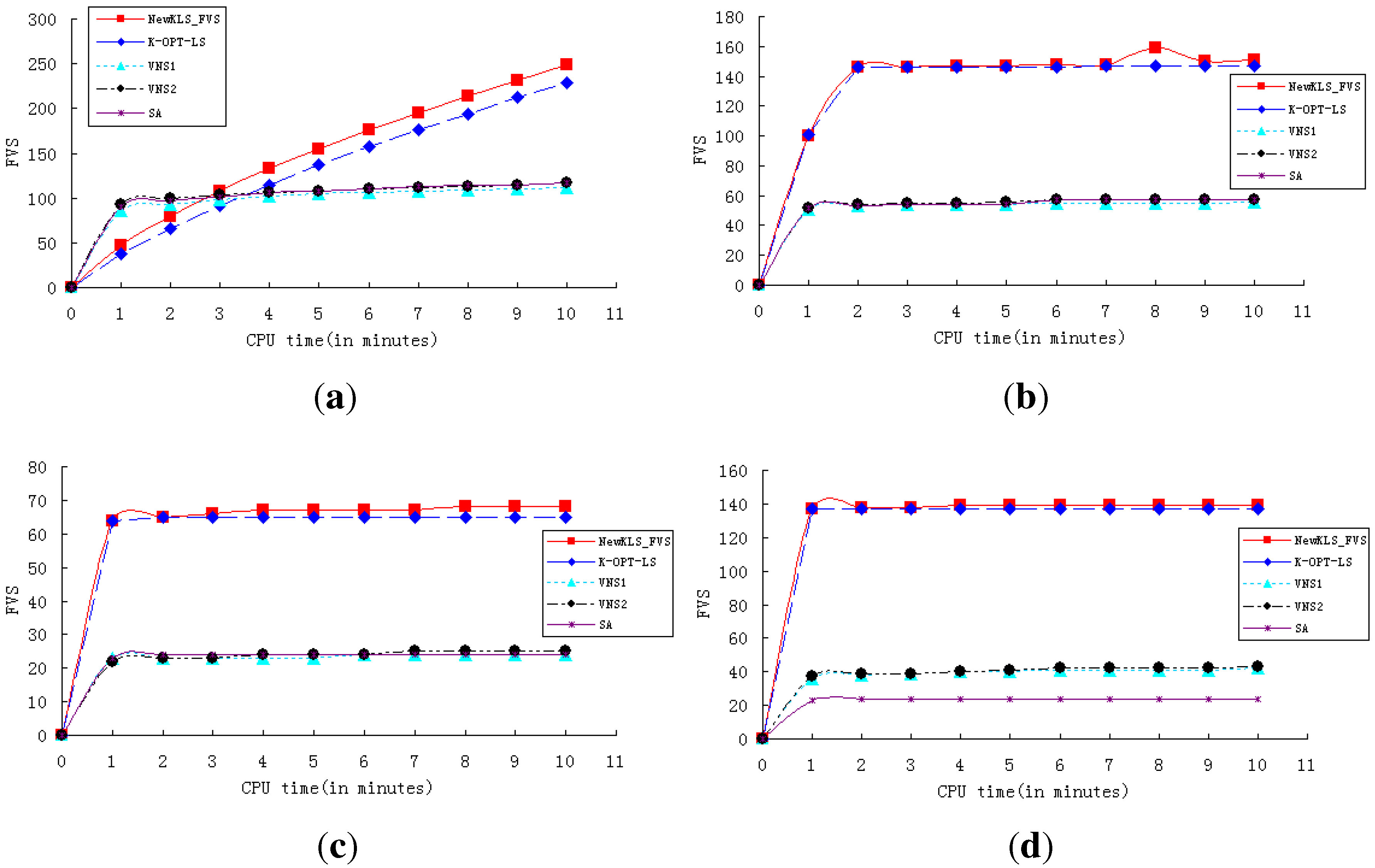
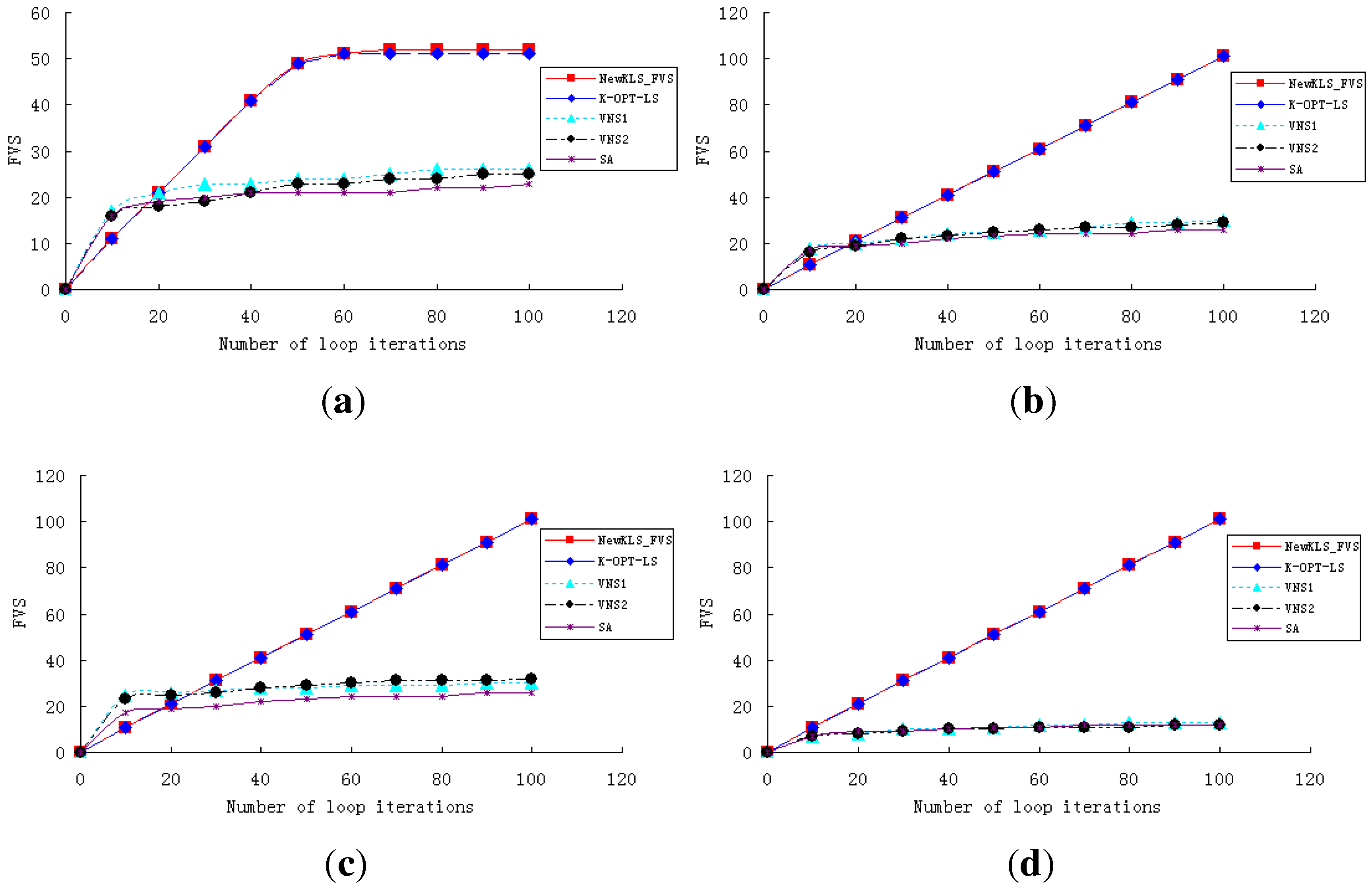
In order to show the performance and efficiency of various algorithms, experiments are conducted to test the algorithms (NewkLS_FVS, k-opt-LS, VNS1, VNS2, SA) on graphs huck.col, inithx.i.1.col, le450_25a.col, zeroin.i.1.col and school1_nsh.col. The convergence curves of these algorithms are reported on both running times (with a CPU-time limit of 10 min; see
Figure 1) and iteration numbers (within 100 iterations; see
Figure 2). The experimental results show that NewkLS_FVS outperforms other algorithms on graphs huck.col, le450_25a.col, zeroin.i.1.col and school1_nsh.col almost at any moment. The solution quality is better than any other compared algorithm after 3 min on inithx.i.1.col. Additionally, the solution quality of NewkLS_FVS is better than those of any other compared algorithm on all tested graphs after 20 iterations. It can be seen that the performance of the algorithm, k-opt-LS, is better than VNS1, VNS2 and SA on almost all these instances, and the convergence performance of k-opt-LS is improved by using the proposed approaches.
Figure 1.
Comparison of the algorithms with a CPU-time limit of 10 min. (a) inithx.i.1.col; (b) le450_25a.col; (c) school1_nsh.col; (d) zeroin.i.1.col.
Figure 1.
Comparison of the algorithms with a CPU-time limit of 10 min. (a) inithx.i.1.col; (b) le450_25a.col; (c) school1_nsh.col; (d) zeroin.i.1.col.
Figure 2.
Comparison of the algorithms within 100 iterations. (a) huck.col; (b) inithx.i.1.col; (c) le450_25a.col; (d) zeroin.i.1.col.
Figure 2.
Comparison of the algorithms within 100 iterations. (a) huck.col; (b) inithx.i.1.col; (c) le450_25a.col; (d) zeroin.i.1.col.
5.4. Evaluation of the Algorithms
From the report of
Table 3,
Table 4,
Table 5,
Table 6 and
Table 7, it can be seen that the results of NewKLS_FVS and k-opt-LS are obviously better than those of VNS1, VNS2 and SA.
Table 8 presents the results of the best algorithm for each instance testing DIMACS. In
Table 8, the column
best means the best result from the algorithms, and the column
worst is the worst result from the algorithms. The column
the-best-algorithm is the set of algorithms capable of obtaining the best result.
Table 8.
Results for algorithm analysis.
Table 8.
Results for algorithm analysis.
| Instance | Best | Worst | The-Best-Algorithm |
|---|
| anna.col | 126 | 126 | a,b |
| david.col | 66 | 66 | a,b |
| DSJC125.1.col | 58 | 58 | a |
| DSJC125.5.col | 15 | 15 | a,b |
| DSJC125.9.col | 6 | 6 | a,b,c,d |
| fpsol2.i.1.col | 366 | 364 | a |
| fpsol2.i.2.col | 370 | 370 | a |
| fpsol2.i.3.col | 344 | 344 | a,b |
| games120.col | 47 | 46 | a,b |
| homer.col | 520 | 520 | a,b |
| huck.col | 52 | 52 | a,b |
| inithx.i.1.col | 602 | 554 | a |
| inithx.i.2.col | 549 | 548 | a |
| inithx.i.3.col | 529 | 529 | a |
| jean.col | 63 | 63 | a,b |
| latin_square_10.col | 13 | 13 | a |
| le450_5a.col | 114 | 108 | a |
| le450_5b.col | 114 | 109 | a |
| le450_5c.col | 104 | 94 | a |
| le450_5d.col | 104 | 97 | a |
| le450_15b.col | 129 | 126 | a |
| le450_15c.col | 66 | 63 | a |
| le450_15d.col | 67 | 65 | a |
| le450_25a.col | 157 | 154 | a |
| le450_25b.col | 141 | 138 | a |
| le450_25c.col | 78 | 76 | a |
| le450_25d.col | 72 | 70 | a |
| miles250.col | 81 | 80 | a |
| miles500.col | 43 | 43 | a,b |
| miles750.col | 27 | 27 | a,b |
| miles1000.col | 20 | 20 | a,b |
| miles1500.col | 10 | 10 | a,b |
| mulsol.i.1.col | 121 | 121 | a,b |
| mulsol.i.2.col | 133 | 133 | a,b |
| mulsol.i.3.col | 129 | 129 | a,b |
| mulsol.i.4.col | 130 | 130 | a,b |
| mulsol.i.5.col | 131 | 131 | a,b |
| myciel3.col | 8 | 8 | a,b |
| myciel4.col | 16 | 16 | a,b |
| myciel6.col | 61 | 61 | a,b |
| myciel7.col | 122 | 122 | a |
| queen5_5.col | 7 | 7 | a,b,c,d,e |
| queen6_6.col | 9 | 9 | a,b,c,d,e |
| queen7_7.col | 11 | 11 | a,b,c,d |
| queen8_8.col | 13 | 13 | a,b |
| queen8_12.col | 16 | 16 | a,b |
| queen9_9.col | 14 | 14 | a,b |
| queen10_10.col | 16 | 16 | a,b |
| queen11_11.col | 18 | 18 | a,b |
| queen12_12.col | 20 | 19 | a,b |
| queen13_13.col | 21 | 21 | a,b |
| queen14_14.col | 23 | 22 | a,b |
| queen15_15.col | 25 | 24 | a,b |
| queen16_16.col | 26 | 25 | a,b |
| school1.col | 77 | 75 | a |
| school1_nsh.col | 71 | 67 | a |
| zeroin.i.1.col | 139 | 139 | a |
| zeroin.i.2.col | 160 | 160 | a |
| zeroin.i.3.col | 156 | 156 | a |
Table 8 shows that NewKLS_FVS obtains the best result for all the tested instances, and k-opt-LS obtains 34 best results. From the report, it can be seen that they both perform better than other test procedures for the feedback vertex set problem.
6. Concluding Remarks
This paper addresses an NP-complete problem, the feedback vertex set problem, which is inspired by many applications, such as deadlock detection in operating systems and relational database systems of an operating system. An efficient local search algorithm, NewkLS_FVS, is proposed to solve this problem, and it was compared with popular heuristics, such as variable depth search and simulated annealing. From the experiments on random graphs and DIMACS benchmarks, it can be seen that NewkLS_FVS is able to obtain better solutions than the variable depth search, and it has good performance by setting the parameter, tabu tenure, to a suitable value.


