
High-Order Entropy Compressed Bit Vectors with Rank/Select

1
Institut für Theoretische Informatik, Karlsruhe Institute of Technology, Kaiserstraße 12, 76131 Karlsruhe, Germany
2
Fakultät für Informatik, Technical University of Dortmund, Otto-Hahn-Straße 14,44227 Dortmund, Germany
*
Author to whom correspondence should be addressed.
Algorithms 2014, 7(4), 608-620; https://0-doi-org.brum.beds.ac.uk/10.3390/a7040608
Submission received: 21 August 2014
/
Revised: 8 October 2014
/
Accepted: 28 October 2014
/
Published: 3 November 2014
Abstract
:We design practical implementations of data structures for compressing bit-vectors to support efficient rank-queries (counting the number of ones up to a given point). Unlike previous approaches, which either store the bit vectors plainly, or focus on compressing bit-vectors with low densities of ones or zeros, we aim at low entropies of higher order, for example . Our implementations achieve very good compression ratios, while showing only a modest increase in query time.
1. Introduction
Bit vectors are ubiquitous in data structures. This is even more true for succinct data structures, where the aim is to store objects from a universe of size u in asymptotically optimal bits. The best example are succinct trees on n nodes, which can be represented by parentheses in optimal bits, while allowing many navigational operations in optimal time [1].
Bit vectors often need to be augmented with data structures for supporting rank, which counts the number of 1’s up to a given position, and select, which finds the position of a given 1 [2,3,4,5,6]. Often, the bit-vectors are compressible, and ideally this compressibility should be exploited. To the best of our knowledge this has so far been done mostly for sparse bit-vectors [4,5]. For other kinds of regularities, we are only aware of two recent implementations [7,8], which are, however, tailored towards bit vectors arising in specific applications (FM-indices [8] and wavelet trees on document arrays [7]), though they may also be effective in general.
1.1. Our Contribution
We design practical implementations for compressing bit-vectors for rank- and select-queries that are compressible under a different measure of compressibility, namely bit-vectors having a low empirical entropy of order (see Section 2 for formal definitions). Our algorithmic approach is to encode fixed-length blocks of the bit-vector with different kinds of codes (Section 3.1). While this approach has been theoretically proposed before [9], we are not aware of any practical evaluations of this scheme in the context of bit-vectors and rank-/select-queries. An interesting finding (Section 3.2) is that we can show that the block sizes can be chosen rather large (basically only limited by the CPU’s word size), which automatically lowers the redundancy of the (otherwise incompressible) rank-information. We focus on data structures for rank, noting that select-queries can either be answered by binary searching over rank-information, or by storing select-samples in nearly the same way as we do for rank [10].
We envision at least two possible application scenarios for our new data structures: (1) compressible trees [11], where the bit-vectors are always dense (same number of opening and closing parentheses), but there exist other kinds of regularities. Easy examples are stars and paths, having balanced parentheses representations and , respectively. (2) wavelet trees on repetitive collections of strings that are otherwise incompressible, like individual copies of DNA of the same species [7].
2. Preliminaries
2.1. Empirical Entropy
Let T be a text of size n over an alphabet Σ. The empirical entropy of order zero [12] is defined as:
where is the number of occurrences of the symbol c in T. is a lower bound for any compression scheme that encodes each occurrence of a symbol within T into the same code regardless of its context. Using such compression schemes any symbol of the original text can be decoded individually, allowing random access to the text with little overhead. However, only takes into account the relative frequency of each symbol, and so ignores frequent combinations. Much better compression is often possible by taking the context into account.
The empirical entropy of order k is defined as:
where is the concatenation of all symbols in T directly following an occurrence of s.
The empirical entropy of order k is a lower bound for any compressor that requires at most k preceding symbols in addition to the code in order to decode a symbol. We have log ≥ ≥ ≥ … . For texts derived from a natural source is often significantly smaller than even for a quite small k. Thus, is the measure of choice for any context based random access compression scheme.
2.2. Empirical Predictability
Recently, Gagie [13] defined a new complexity measure called empirical predictability. If we are asked to guess a symbol chosen uniformly at random without any context given, our best chance is to guess the most frequent symbol. The probability of a correct prediction is called the empirical predictability of order 0. Now we consider being asked the same question, but we are allowed to read the preceding k bits of context or, if there are not enough preceding bits, the exact symbol. We then call the chance to predict correctly the empirical predictability of order k. It is defined as . (Actually, Gagie [13] adds a summand of for the first k bits of the text. In contrast, we consider k to be a small constant. Considering we can omit this summand for both empirical entropy and empirical predictability.) Note that . If is high we intuitively expect a compressed version of the text to be small. This is inverse to the other complexity measures, where we need a low value to get a small compressed text. In fact, we prove:
Lemma 1. For binary texts () the empirical entropy is an upper bound for .
Proof. Let k be fixed. For let be the number of correct predictions after reading s and the number of incorrect predictions after reading s.
To simplify notation we assume . Then:
which proves the claim. ☐
Note that we omitted some significant terms; the actual should be even lower. This relation between the empirical entropy and the empirical predictability had not been established before. Lemma 1 will be used in Section 4, since there the test data generator mimics the process of empirical predictability; but we think that the lemma could also have different applications in the future.
2.3. Succinct Data Structures for Rank
Let be a bit-string of length n. The fundamental rank- and select-operations on T are defined as follows: gives the number of 1’s in the prefix , and gives the position of the i’th 1 in T, reading T from left to right (). Operations and are defined similarly for 0’s.
In [2,3] Munro and Clark developed the basic structure to solve rank/select queries in constant time within space. Most newer rank/select dictionaries are based on their work, and so is ours. We partition the input bit string into large blocks of length . For each large block we store the number of 1’s before the block, which is equal to a rank sample at the block border. As there are large blocks and we need at most bits to store each of those values, this requires only bits of storage. We call this the top-level structure.
Similarly, we partition each large block into small blocks of size . For each small block we store the number of 1’s before the small block and within the same large block, which is equal to a rank sample relative to the previous top-level sample. As there are small blocks and we need at most bits, this requires only bits of storage. We call this the mid-level structure.
As the size of small blocks is limited to , there are different small blocks possible. Note that not all possible small blocks necessarily occur. For every possible small block and each position within a small block we store the number of 1’s within this small block before the given position in a table. This table requires bits. We call this table the lookup table.
For each small block we need to find the index of the corresponding line in the lookup table. This is, in fact, the original content of the block, and we get it from the text T itself. As we intend to solve this problem with something different than a plain storage of T, we call the representation of T the bottom-level structure. If we use an alternative bottom-level structure the rank structure can still simulate T for constant time read-only random access.
3. New Data Structure
As described in the previous section, rank/select dictionaries break down into top-level, mid-level, bottom-level, and a lookup table. While the top and mid-level structures basically contain rank/select information, the text T is stored in the bottom-level and the lookup table. In fact the bottom-level and the lookup table are sufficient to reconstruct T. Thus we try to exploit the compressibility of T here.
The mid-level structure conceptually partitions T into blocks, which are then used to address the lookup table. Thus the most native approach to compress the bottom-level is to encode frequent blocks into short code words. Using the shortest code for the most frequent blocks produces the best possible compression. Amongst such block encoding techniques is the Canonical Code (Section 3.1.1). However, it produces variable length code words and thus we do not have an easy constant time random access (though this is possible with a bit of work). In order to provide constant time random access we investigate three approaches. Two of them are totally independent of the used code and differ in size and speed. The third one is a code that tries to get fixed length codes in most cases while using small auxiliary data structures for the exceptions. We call it the Exception Code.
The upper-level rank structures already contain the information of how many 1’s a desired block contains. Considering this, a block’s code does not need to be unique amongst all blocks, but only unique amongst all blocks with the same number of 1’s. The actual unique code of a block b then is the pair , where is the number of 1’s in b, and is the stored code word. is calculated for every separately, and we require a decoding table for each , but all code words can be stored in the same data structure. Note that we still only have one decoding table entry per occurring block, and thus memory consumption only increases by . This is done for each of the codes in Section 3.1.
3.1. Coding Schemes
3.1.1. Canonical Code
This coding scheme corresponds to the idea of Ferragina and Venturini [9], where it is also shown that the coding achieves empirical entropy of order k. It works as follows. We order all possible bit strings by their length and, as secondary criterion, by their binary value. We get the following sequence: . Note that we can calculate the position j of a bit string s in this sequence: , where is the bit string s with a preceding 1, interpreted as a binary number. We use the first element of this sequence to encode the most frequent block, the second one for the second most frequent block, etc. This is obviously optimal in terms of memory consumption as long as we assume the beginnings and endings of code words to be known.
As long as each block is encoded in a code of fixed length b the code of a specific block i can be found by simple arithmetic. However, the Canonical Code produces variable length code words and thus we require a technique to find the desired block code. We next describe two approaches to achieve that.
One option is to maintain a two-level pointer structure [9], similar to the top and mid-level of the rank directory described in Section 2.3. For each large block we store the beginning of its first encoded small block directly in bits using bits in total. We call it the top-level pointers. The mid-level pointers defined analogously and use bits. As for rank structures this only requires constant time to access, but the space consumption is much more significant than the indicates.
An alternative approach is to store a bit vector parallel to the encoded bit vector, where we mark the beginning of each code word with a 1 and prepare it for select queries (as previously done in [14,15], for example). To find the ith code word we can use on this beginnings vector V. If the original text is highly compressible, the encoded bit vector and thus the beginnings vector is rather short compared to other data structures used. Otherwise, it is sparsely populated and can be compressed by choosing an appropriate select dictionary, for example the sparse array by Sadakane and Okanohara [5]. On the downside, using select to find the proper code word comes with constant but significant run-time costs in practice.
3.1.2. Exception Code
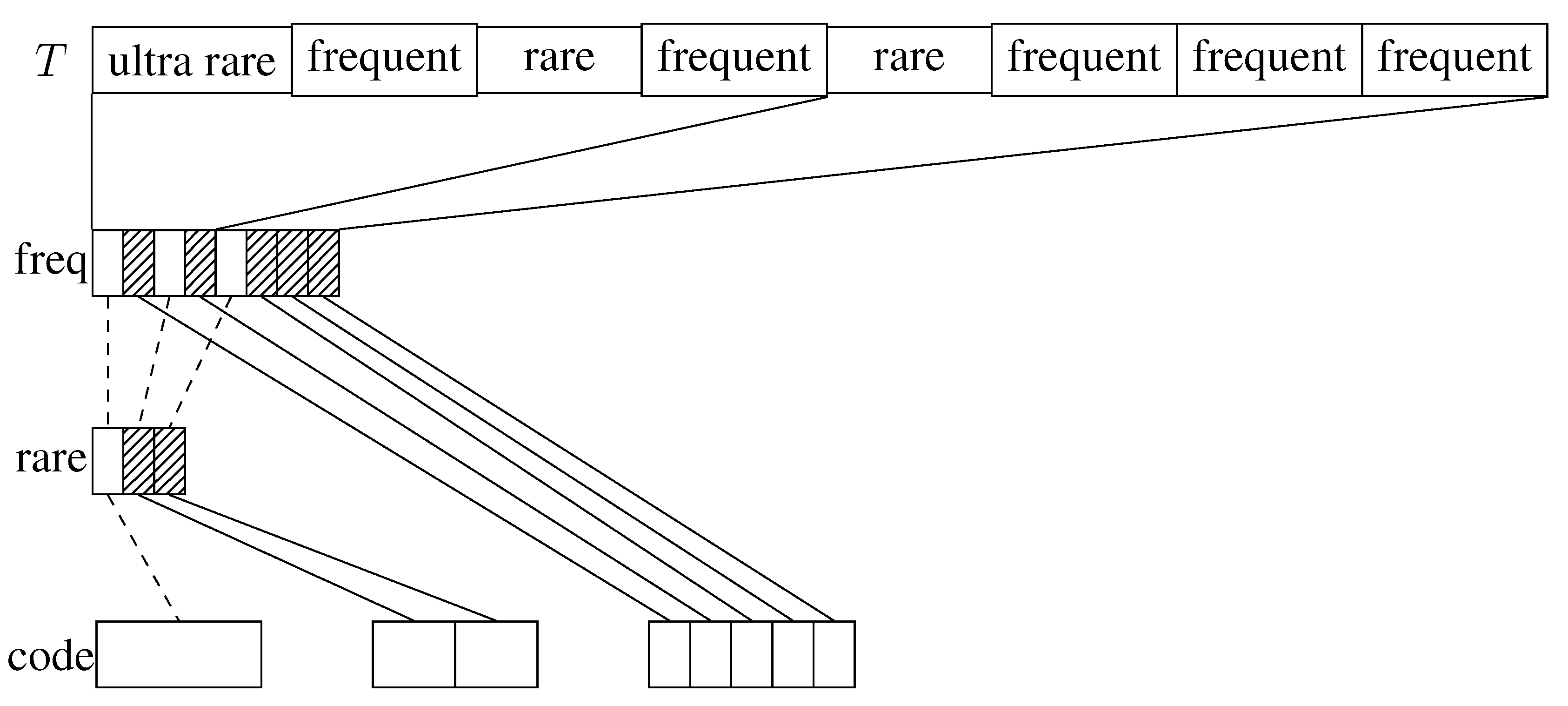
For this code we categorize the blocks into 3 classes (see also [16] for the a generalization of this idea called alphabet partitioning): frequent blocks, rare blocks and ultra rare blocks. For the first two classes we choose parameters and , defining how many bits we use to encode their blocks. Ultra rare blocks are stored verbatim, so they still need their original size . We define the most frequent blocks to be frequent blocks. Rare blocks are the most frequent blocks that are not yet classified as frequent. All other blocks are classified ultra rare.
We maintain simple arrays for each of those classes of blocks, encoding all blocks of that class in the order of their occurrence. In order to access a block we need to find out what class it belongs to and how many blocks of that class occur before. For this we maintain a bit vector with one bit per block. We mark frequent blocks with a 1 and prepare it for rank queries using an appropriate rank dictionary. Those rank queries tell us how many frequent blocks occur before a desired block, so it is already sufficient for accessing frequent blocks. For non-frequent blocks subtracting the number of previous frequent blocks from its index we obtain its position in a conceptional list of non-frequent blocks. With this we can proceed exactly the same way as above: maintaining a bit vector with one bit per non-frequent block marking rare blocks with a 1 and preparing it for rank queries. To access a non-frequent block we need to rank it both in and in . Figure 1 illustrates the data structures.
The Exception Code uses more space than the Canonical Code for the encoded blocks, and it is not clear at all if it achieves kth order empirical entropy in theory. However, the former only requires two rank structures on and to enable random access. As they are built upon bit vectors with only one bit per block, they require at most bits for blocks of size b, and our hope is that this is small compared to the beginnings vector or even the two-level pointer structure required for the Canonical Code structure. In terms of execution time we need little more than one subordinate rank query for frequent blocks, and two for non-frequent blocks, hopefully resulting in faster average query times.
Figure 1.
Illustration to the Exception Code. Shaded blocks denote 1’s, and empty blocks 0’s.

3.2. Table Lookup
3.2.1. Verbatim Lookup vs. Broadword Computation
In the original Munro and Clark version as described in Section 2.3, the lookup table stores the relative rank or select results for each of the possible small blocks and each of the possible queries in bits requiring bits of storage. To keep the table small, had to be chosen very small. Vigna [6] bypasses the lookup table and instead calculates its entries on the fly via broadword computation. According to Vigna [6], “broadword programming uses large (say, more than 64-bit wide) registers as small parallel computers, processing several pieces of information at a time.” This is efficient as long as blocks fit into processor registers. In our approach bottom-level blocks are encoded only based on their frequency, and not on their content. Thus we inevitably need a decoding table. After looking up the appropriate table row it needs to provide rank information. This can be stored directly within the table, turning it into a combined decoding and lookup table.
3.2.2. Expected Table Size
In the rank/select structure as described in Section 2.3, all possible small blocks are listed. This implies that has to be small, which increases the number of small blocks. In our structure the lookup table only contains blocks that do actually occur in T. (This is possible since both of the codes above—Canonical Code and Exception Code—imply an implicit enumeration of the occurring blocks without gaps; see, for example, the first paragraph of Section 3.1.1 for how to compute this numbering.) Thus the table size is limited by , without restricting the choice of . For predictable texts (), we intuitively expect most blocks to occur very often within T (and thus not increasing the lookup table size). This intuition is confirmed in the following, by calculating the expected number of entries in the lookup table.
To this end, look at a fixed block of bits. Its probability of occurrence depends mainly on the number i of bits that are not as predicted. Assuming the first k bits are distributed uniformly at random, the probability of B (with i mispredictions) to occur is:
There are
blocks with i mispredictions, so we expect
of them to appear within T. This is the well known formula of bounded exponential growth, a monotonic concave function bounded from above by . Its derivative is proportional to the satiation , and . For small i the upper bound is quite small. For larger i the growth rate quickly falls behind the linear growth of other data structures used. Summing over all possible i, we get the expected number of blocks occurring in the lookup table:
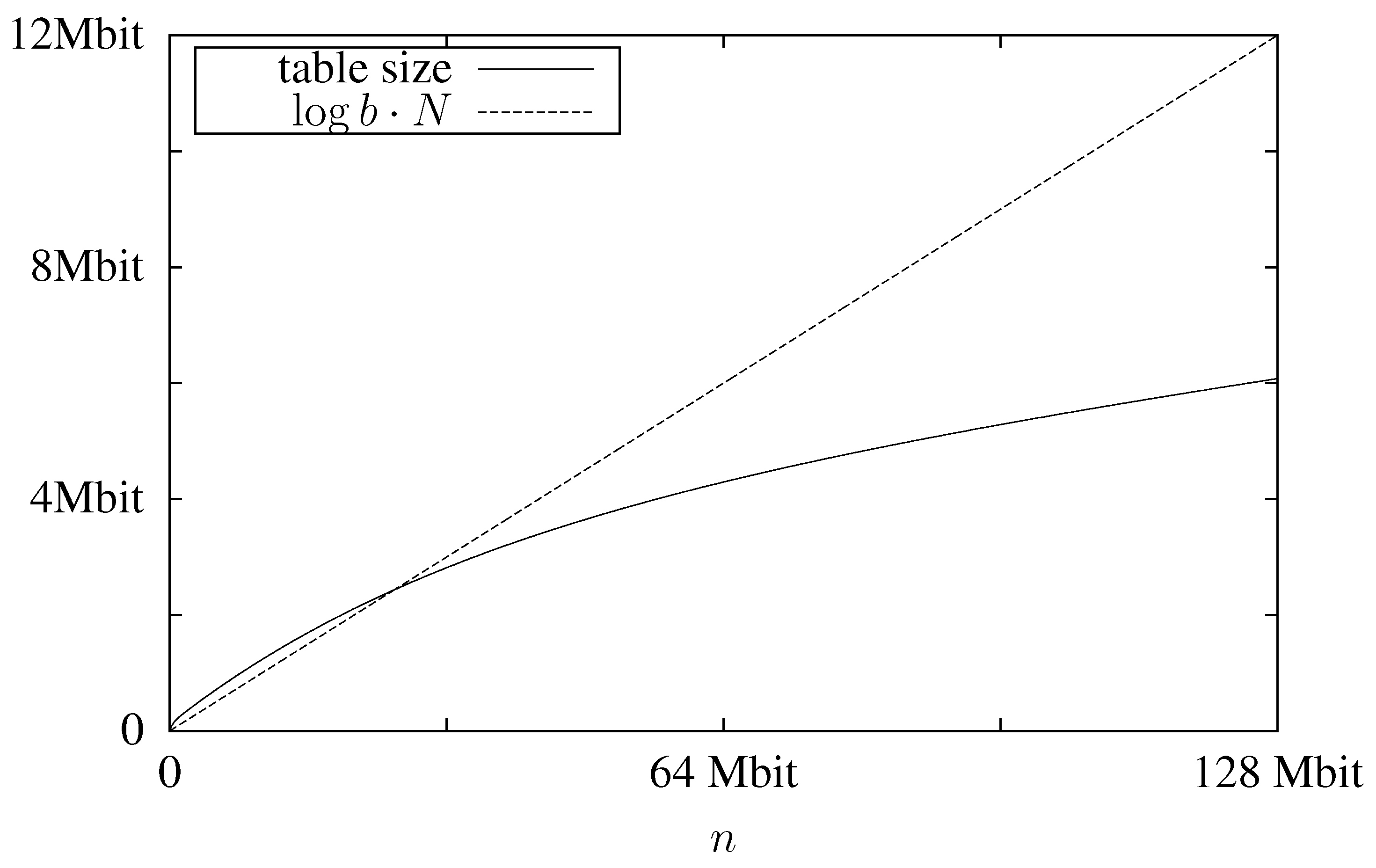
In Figure 2 we plot the expected table size, which is , using and as an example. For comparison we also plot , which is a lower bound for the mid-level data structure. We can see that despite the large block size the table’s memory consumption is less than that of the mid-level data structure. As the lookup table is the only data structure that grows with increasing block sizes and the mid-level structure significantly profits from large block sizes, this shows that has to be chosen quite high.
Figure 2.
Expected memory usage for the lookup table for a text with and block size .

4. Test Data Generator
Our data structures aim to fit data with low empirical entropy of higher order even if the empirical entropies of lower order are quite high. We created such data by a specific generator that we are going to describe next, which might be of independent interest. It produces bit vectors with lower order empirical entropies very close to 1 () and higher order empirical entropies significantly lower ().
The test data generator rolls each bit with a probability for a 1 dependent on , where are the k preceding bits. We get these probabilities from a table. The first half of this table, containing probabilities for bit patterns starting with a 0, is filled with values close to 1 or close to 0 at random. By Lemma 1 and since our test data generator mimics the empirical predictability, this ensures a low . The second half is filled with exactly the opposite probabilities namely for all bit patterns s of length . This ensures lower order empirical entropies to be 1, as shown in Lemma 2 below.
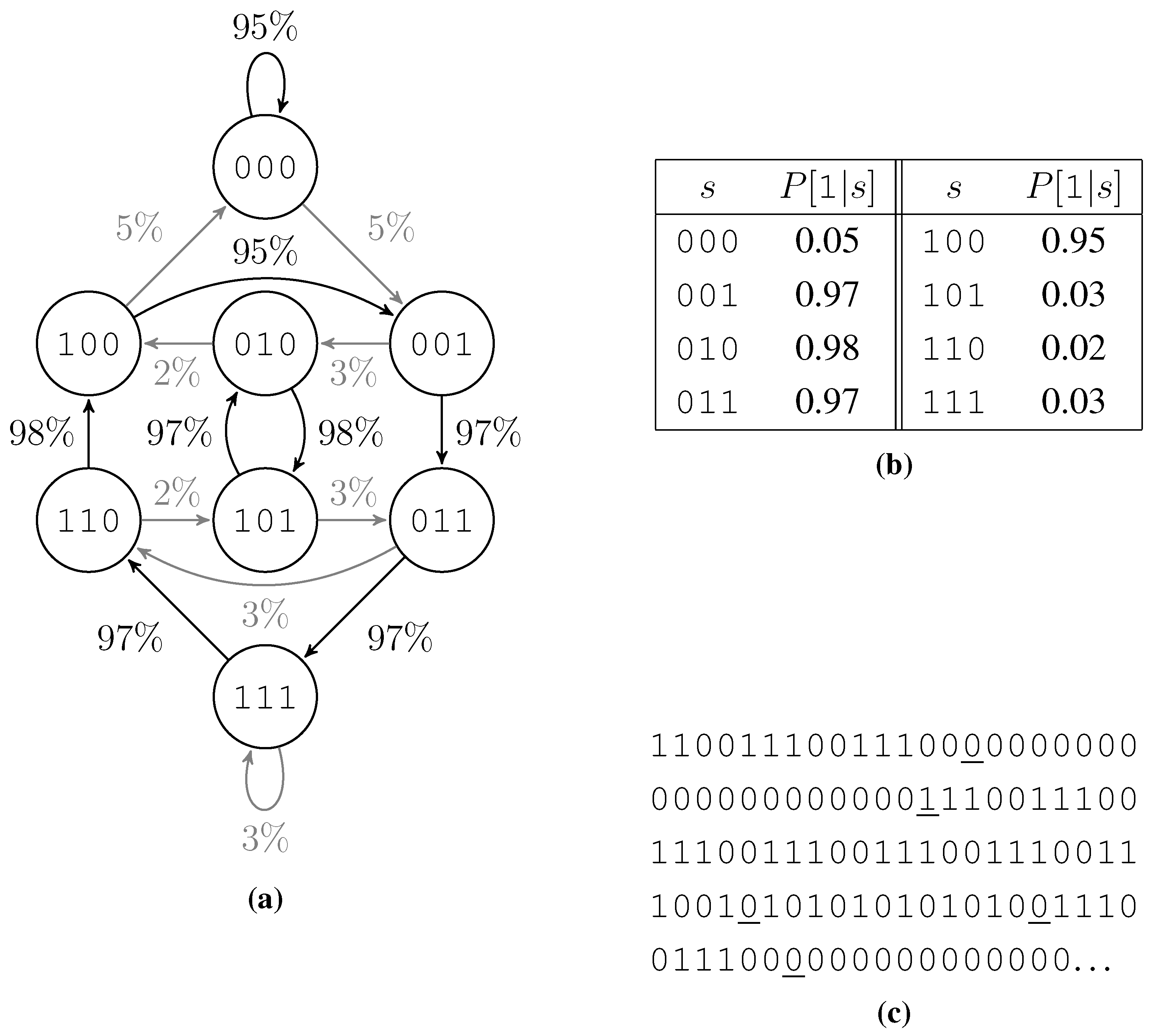
From a different point of view this test data generator is a probabilistic finite state machine with one state for each bit pattern of length k and two state transitions out of each state, one with high probability and one with low probability. Due to filling the second half of the table opposite to the first, the two incoming state transitions of each state behave like the outgoing ones: One of them has a high probability and the other has a low probability. Thus we get circles of high probability edges and a low probability to switch the circle or jump within a circle. Figure 3 shows such a finite state machine, the according probability table, and an example output bit string.
Figure 3.
Example of a test data generation. (a) The associated finite state machine, low probability edges are shown gray. (b) Table of probabilities to roll a 1. (c) Output, low probability rolls are underlined.
Figure 3.
Example of a test data generation. (a) The associated finite state machine, low probability edges are shown gray. (b) Table of probabilities to roll a 1. (c) Output, low probability rolls are underlined.

Lemma 2. An infinite text generated that way has .
Proof. We have to show that the finite state machine enters each state with the same probability in the long term, thus we have to show that the uniform distribution vector is an eigenvector of the state transition matrix of the Markov process. For each we have:
as this holds for all , we get , which proves the claim. ☐
Lemma 2 also holds for finite texts except for statistical errors, which are negligible for long enough texts.
5. Experimental Results
We implemented the data structures described in this article in C++ and made extensive tests tuning the parameters. The source code is available at [17]. We used GNU g++ 4.6.3 with the flags -O3 -funroll-loops -DNDEBUG -std=c++0x to compile our programs. Our test computer was an Intel [email protected] GHz with 32 kiB L1-, 256 kiB L2-, and 4 MiB L3-cache and 8 GiB RAM. Interestingly, tuning for space also resulted in faster query times, mainly due to caching effects. This resulted in the following implementations:
canRnk2LPTR A basic 2-level structure, using the Canonical Code from Section 3.1. Backed by the analysis of the expected table size (Section 3.2), we used large block sizes on both levels, namely and .
canRnkBeg The same as canRnk2LPTR, but this time using a bit-vector marking the beginnings of the codewords.
exceptionRank The Exception Code from Section 3.1, using parameters , , , and .
We compare our data structures to several existing implementations of rank and select dictionaries from different sources. We stress that none of these data structures was designed to achieve high order compression; we just include them in our tests to give some idea of how our new structures compare with existing implementations.
sdslMcl Munro and Clark’s original rank-dictionary, using an implementation from Simon Gog’s sdsl [18].
sdslv5 A space-conscious rank implementation from sdsl, tuned to use only 5% of space on top of the bit vector.
rsdicRRR A 0-order compressed version of Navarro and Providel’s rank-dictionary [10], using an implementation by Daisuke Okanohara [19].
SadaSDarray Okanohara and Sadakane’s SDArray [5].
suxVignaRank9 Sebastiano Vigna’s rank9-implementation [6].
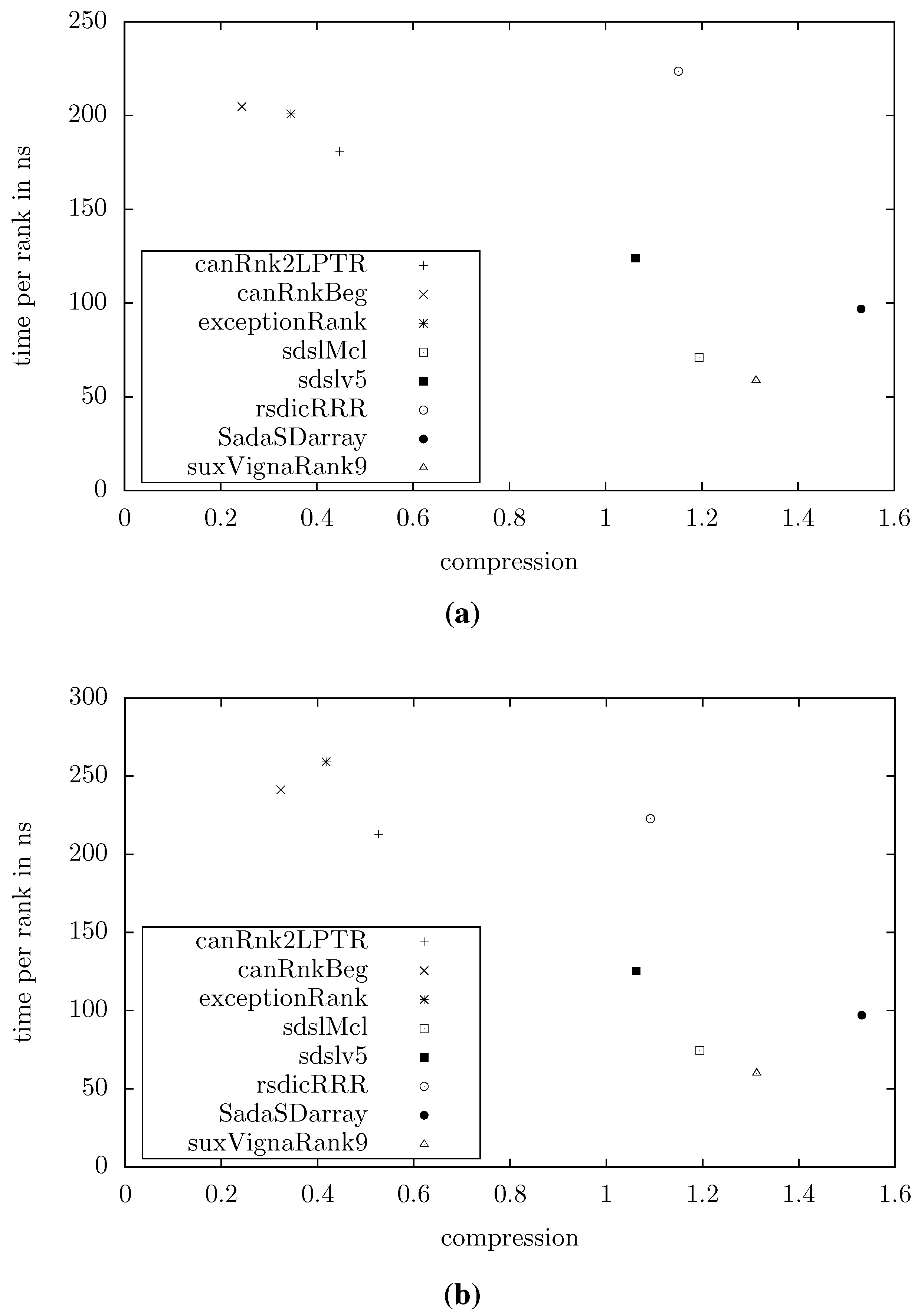
Figure 4 shows the compression and query times for example texts with MB and or , respectively (averaged over 10 repeats of random queries). Other distributions of entropies yielded similar results. We can see that our data structures are significantly smaller than the others. At the extreme end, our smallest structure (canRnkBeg) uses less that 1/4 of the space used by the smallest existing structure (sdslv5). However, we trade this advantage for higher query times, in the example mentioned by a factor of 2.
Figure 4.
Space/time tradeoff for various rank dictionaries. (a) , for . (b) , for .

6. Conclusions
We introduced new methods for compressing dense bit-vectors, while supporting rank/select queries, and showed that the methods perform well in practice. An interesting extension for future work is engineering compressed balanced parentheses implementations, with full support for all navigational operations.
Author Contributions
Both authors developed the algorithms and wrote the manuscript. Implementation and testing was done by Kai Beskers.
Conflicts of Interest
The authors declare no conflict of interest.
References
- Sadakane, K.; Navarro, G. Fully-Functional Succinct Trees. In Proceedings of Twenty-First Annual ACM-SIAM Symposium on Discrete Algorithms, Austin, TX, USA, 17–19 January 2010; pp. 134–149.
- Clark, D. Compact Pat Trees. PhD thesis, University of Waterloo, Ontario, Canada, 1996. [Google Scholar]
- Munro, J.I. Tables. In Proceedings of 16th Foundations of Software Technology and Theoretical Computer Science, Hyderabad, India, 18–20 December 1996; pp. 37–42.
- Raman, R.; Raman, V.; Rao, S.S. Succinct indexable dictionaries with applications to encoding k-ary trees and multisets. In Proceedings of the Thirteenth Annual ACM-SIAM Symposium on Discrete Algorithms, San Francisco, CA, USA, 6–8 January 2002; pp. 233–242.
- Okanohara, D.; Sadakane, K. Practical Entropy-Compressed Rank/Select Dictionary. In Proceedings of the Ninth Workshop on Algorithm Engineering and Experiments, New Orleans, LA, USA, 6 January, 2007.
- Vigna, S. Broadword implementation of rank/select queries. In Experimental Algorithms; Springer: Berlin Heidelberg, Germany, 2008; pp. 154–168. [Google Scholar]
- Navarro, G.; Puglisi, S.J.; Valenzuela, D. Practical compressed document retrieval. In Experimental Algorithms; Springer: Berlin Heidelberg, Germany, 2011; pp. 193–205. [Google Scholar]
- Kärkkäinen, J.; Kempa, D.; Puglisi, S.J. Hybrid Compression of Bitvectors for the FM-Index. In Proceedings of Data Compression Conference, Snowbird, UT, USA, 26–28 March 2014; pp. 302–311.
- Ferragina, P.; Venturini, R. A Simple Storage Scheme for Strings Achieving Entropy Bounds. In Proceedings of the Eighteenth Annual ACM-SIAM Symposium on Discrete Algorithms, New Orleans, LA, USA, 7–9 January, 2007; pp. 690–696.
- Navarro, G.; Providel, E. Fast, small, simple rank/select on bitmaps. In Experimental Algorithms; Springer: Berlin Heidelberg, Germany, 2012; pp. 295–306. [Google Scholar]
- Jansson, J.; Sadakane, K.; Sung, W.K. Ultra-succinct representation of ordered trees with applications. J. Comput. Syst. Sci. 2012, 78, 619–631. [Google Scholar] [CrossRef]
- Manzini, G. An Analysis of the Burrows-Wheeler Transform. J. ACM 2001, 48, 407–430. [Google Scholar] [CrossRef]
- Gagie, T. A Note on Sequence Prediction over Lage Alphabets. Algorithms 2012, 5, 50–55. [Google Scholar] [CrossRef]
- Brisaboa, N.R.; Ladra, S.; Navarro, G. DACs: Bringing Direct Access to Variable-Length Codes. Inf. Process. Manag. 2013, 49, 392–404. [Google Scholar] [CrossRef]
- Fischer, J.; Heun, V.; Stühler, H.M. Practical Entropy Bounded Schemes for O(1)-Range Minimum Queries. In Proceedings of Data Compression Conference, Snowbird, UT, USA, 25–27 March 2008; pp. 272–281.
- Barbay, J.; Claude, F.; Gagie, T.; Navarro, G.; Nekrich, Y. Efficient Fully-Compressed Sequence Representations. Algorithmica 2014, 69, 232–268. [Google Scholar] [CrossRef]
- Source code. Available online: http://ls11-www.cs.uni-dortmund.de/_media/fischer/research/diplcode.tar.gz (accessed on 30 October 2014).
- Simon Gog’s sdsl. Available online: https://github.com/simongog/sdsl (accessed on 30 October 2014).
- Daisuke Okanohara’s Rsdic. Available online: https://code.google.com/p/rsdic/ (accessed on 30 October 2014).
© 2014 by the authors; licensee MDPI, Basel, Switzerland. This article is an open access article distributed under the terms and conditions of the Creative Commons Attribution license (http://creativecommons.org/licenses/by/4.0/).
Share and Cite
MDPI and ACS Style
Beskers, K.; Fischer, J. High-Order Entropy Compressed Bit Vectors with Rank/Select. Algorithms 2014, 7, 608-620. https://0-doi-org.brum.beds.ac.uk/10.3390/a7040608
AMA Style
Beskers K, Fischer J. High-Order Entropy Compressed Bit Vectors with Rank/Select. Algorithms. 2014; 7(4):608-620. https://0-doi-org.brum.beds.ac.uk/10.3390/a7040608
Chicago/Turabian StyleBeskers, Kai, and Johannes Fischer. 2014. "High-Order Entropy Compressed Bit Vectors with Rank/Select" Algorithms 7, no. 4: 608-620. https://0-doi-org.brum.beds.ac.uk/10.3390/a7040608