Neural Networks for Muscle Forces Prediction in Cycling

Abstract

This paper documents the research towards the development of a system based on Artificial Neural Networks to predict muscle force patterns of an athlete during cycling. Two independent inverse problems must be solved for the force estimation: evaluation of the kinematic model and evaluation of the forces distribution along the limb. By solving repeatedly the two inverse problems for different subjects and conditions, a training pattern for an Artificial Neural Network was created. Then, the trained network was validated against an independent validation set, and compared to evaluate agreement between the two alternative approaches using Bland-Altman method. The obtained neural network for the different test patterns yields a normalized error well below 1% and the Bland-Altman plot shows a considerable correlation between the two methods. The new approach proposed herein allows a direct and fast computation for the inverse dynamics of a cyclist, opening the possibility of integrating such algorithm in a real time environment such as an embedded application.

1. Introduction

In biomechanics, internal forces exerted during the execution of motor tasks can be estimated by combining a biomechanical model, able to predict the forces acting on each involved joint, with the design of an optimization criterion to determine the contribution of each muscle to the overall force [1]. This approach has been applied in a variety of application fields, ranging from the analysis of gait [2] and running [3], to the study of upper limb movements [4]. For instance, different studies in the literature proposed a biomechanical model of the human shoulder complex, for quasi-static and dynamic estimation of the muscle forces and joint reaction forces in the gleno-humeral joint, combining inverse dynamics and static optimization to estimate the associated muscle forces [5,6,7]. Other studies present a conceptual 3D bipedal nonlinear model for Sit-To-Stand task with optimal controller design for exoskeleton torques [8] or a coupled optimization problem for a 2D model to solve for controller, which shows that central nervous system is able to solve the limb coordination problem when recovering from balance perturbations [9].

In the biomechanics of cycling it is important to evaluate how the athlete executes the required motor task, in order to have objective parameters that quantify the performance [10]. This aspect can be analyzed in terms of power exerted while cycling, using different techniques [11], or investigating the role of muscle activity while performing the task [12,13,14]. To this aim, previous studies proposed an inverse dynamics approach [15,16,17,18] to predict muscle force patterns by the measurement of the external forces exerted on the pedal. These predictions were compared against muscle activity, as estimated from surface Electromyography (sEMG) data [19], after proper preprocessing [20]. The use of standard optimization algorithms, to solve the equations that describe the inverse dynamics of cycling, can represent a limit to the development of a real time device. Being able to estimate muscle forces in real time can be used on the field to assess and monitor athlete performance. The purpose of this study was to develop a new optimization algorithm based on artificial Neural Networks (NN), in order to reduce the computational complexity of the deterministic one used in the previous study [15], while maintaining the quality of estimation.

Concerning the NN, Multilayer Perceptrons (MLP) with a single hidden layer have been proven capable of approximating any function with any desired accuracy, provided that associated conditions are satisfied [21,22,23,24,25]. They are probably the most commonly used NN and have been applied to a wide variety of problems, including function approximation, prediction, and simulation. Although one hidden layer is adequate to enable NN to approximate any given function, some researchers argued that NN with more than one hidden layer might require fewer hidden neurons to approximate the same function. It was theoretically shown in [26] that, given a desired degree of interpolation accuracy, NNs with two hidden layers require considerably fewer hidden neurons compared to NNs with one hidden layer. From a more practical perspective it has been shown in [27], through extensive experiments, that single-hidden-layer NNs are superior to networks with more than one hidden layer with the same level of complexity mainly due to the fact that the latter are more prone to fall into local minima. In engineering applications, there is a clear tendency toward using NNs with only one hidden layer [28]. Generally, feed forward NN have been a natural choice as trainable pattern classifiers because of their function approximation and generalization capabilities [29]. The function approximation capability allows them to form arbitrary nonlinear discriminant surfaces, while the generalization ability allows responding consistently to data never shown to the network itself. In this work, NNs have been used with the aim of obtaining a good approximation of the estimated muscle forces with a reduced computational cost, that represents one of the main targets for real time application in biomedical application [30,31].

2. Methods and Techniques

A biomechanical model was identified to reproduce the cycling task and used for the muscle forces estimation of the lower limb. It has been modeled as a three-joint (i.e. ankle, knee, and hip) system, actuated by nine muscles as shown in Figure 1, and built in three steps:

• Definition of a kinematic model to evaluate the position of every segment of the leg involved in the gesture;
• Definition of the inverse dynamics to evaluate the muscular torque for every joint;
• Calculation of the muscular forces through the data obtained with the two previous steps.

Regarding the third step, a cost function, based on a physiological criterion, was minimized to predict muscular force patterns. This optimization was obtained by using a feed forward NN. An additional one was used to solve the equation associated with the first step, as described in the following.

Figure 1. Lower limb muscles that contributes to cycling involved in the model.

Figure 1. Lower limb muscles that contributes to cycling involved in the model.

Results obtained with this approach were compared to the ones obtained with the previous deterministic approach [15], using Bland-Altman plots, which is widely used in literature to compare different estimation techniques of the same quantity [32,33].

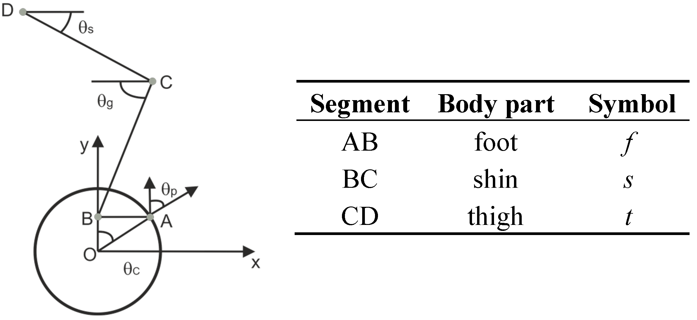
2.1. Biomechanical Model Identification

Restricting the analysis to the sagittal plane, the kinematic model of the lower limb is composed of constrained rigid elements and mechanical elements of the bicycle, used to transmit the motion to the wheel. By modeling each body segment and each mechanical element as a segment (Figure 2) it is possible to define a kinematic chain with five elements and two degrees of freedom, so the position of each member in the sagittal plane is determined by the length of each segment and two of the following angles:

• θ_c, angle between the bicycle’s frame and the crank;
• θ_p, angle between the crank and the pedal;
• θ_g, knee angle identified as in Figure 2;
• θ_s, hip-saddle angle identified as in Figure 2.

Figure 2. Kinematic chain of lower limb and angle between body segment.

Figure 2. Kinematic chain of lower limb and angle between body segment.

The length of each segment of the model was determined by direct measurement. Once kinematic data and pedal forces are obtained—measuring θ_c, and θ_p and calculating the other angles as reported in [15] (θ_s(θ_c, θ_p) and θ_g(θ_s))—ankle, knee and hip joint moments are calculated using the inverse dynamics, using inertial parameters given by literature [34]. Afterwards, these data are used to implement the three equilibrium equations at each joint, involving the following muscles, that represent the minimum set to be involved in the model: (1) Tibialis anterior (TA); (2) Soleus (SO); (3) Gastrocnemius (GA); (4) Vastii (VA); (5) Rectus femoris (RF); (6) Short head of biceps femoris (BFs); (7) Long head of Biceps Femoris (BFl); (8) Iliacus (IL); (9) Gluteus Maximum (GLM). The relation between the muscular moments and the muscular forces at each joint j is given by the equation:

$${\displaystyle \sum }_{i=1}^{N_j}{F}_i \times d_{ij}=M_j$$

(1)

where M_j represents the muscular moment at the j-th joint, N_j is the number of muscles acting on the j-th joint, F_i is the muscular force exerted by the i-th muscle and d_ij is the effective moment arm of the i-th muscle from the j-th joint. The values of muscular moment arms were calculated as a second order function of the joint angle in % of the length of the segment on which muscle belly is located, based on the equation reported in [35]. As the number of equations is not sufficient to calculate muscular force values, these were calculated by minimizing the cost function:

$$U={\displaystyle \sum }_{i=1}^p{\left(\frac{F_i}{PCS{A}_i}\right)}^3$$

(2)

associated with the boundary conditions:

$$0<F_i<F_{imax}$$

(3)

here, given p total number of muscles, and being PCSA_i and F_imax respectively the physiological cross sectional area and the maximum force value for the i-th muscle, obtained by the literature [34]. The cubic exponent used in the equation (3), guarantees the best tradeoff between the muscular contractile force and the maximum duration of the contraction. This cost function is widely used in literature [36,37] as it relies on the co-activation of all the muscles involved in the gesture.

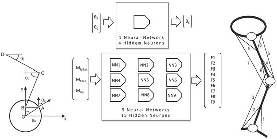
2.2. Neural Network Design

FFNNs (Feed Forward Neural Networks) were trained by the Levenberg–Marquardt algorithm [38], which is a quasi-Newton optimization algorithm designed for nonlinear least squares problems. It is probably the most efficient training algorithm for small and medium-sized NNs [39]. In this work, NNs are used in two critical steps:

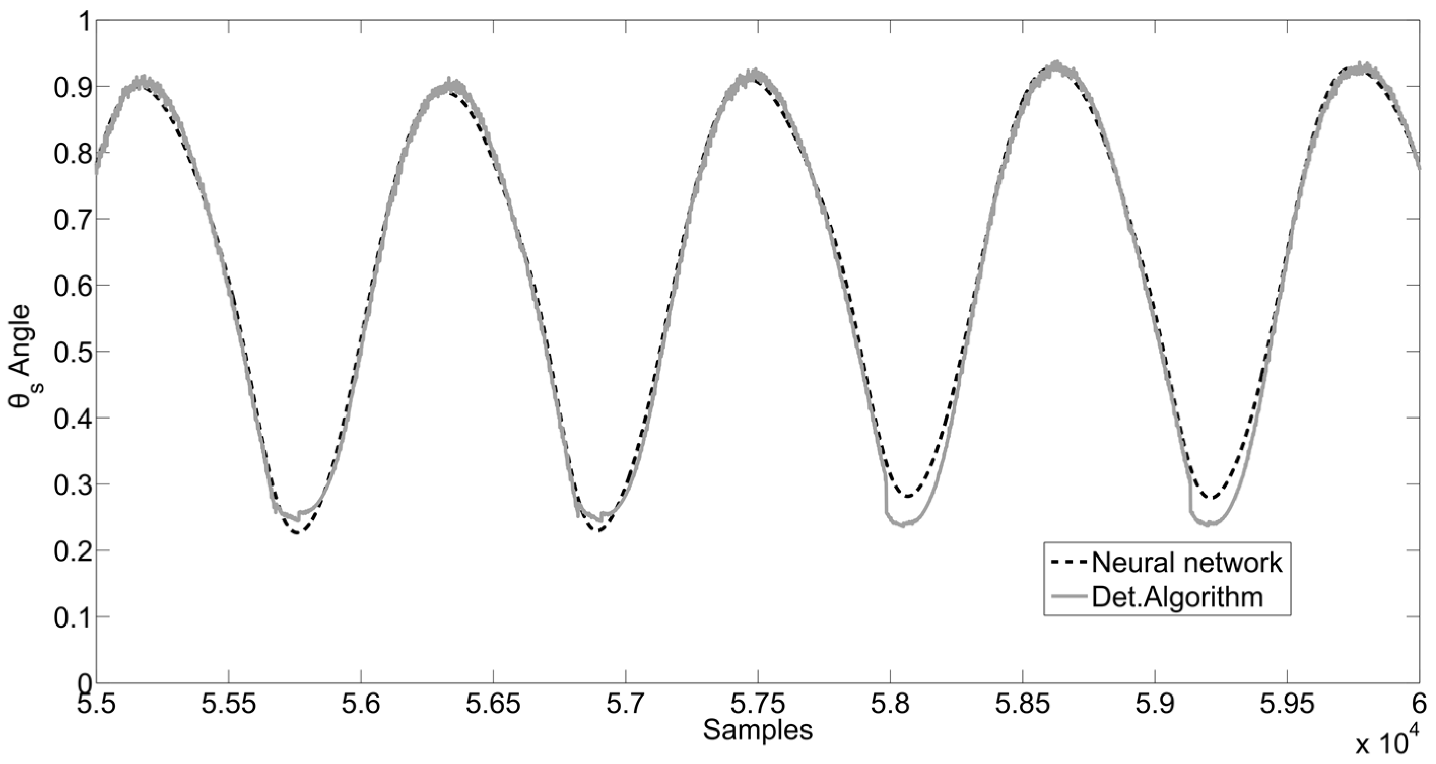
• Calculation of the relative rotational angle between the frame of the bicycle and the thigh, θ_S;
• Estimation of muscle forces.

In the first step, considering the coordinates of the points (A, B, C, D) respect to the reference system centered in O, as reported in Figure 2, the neural network is necessary since the angle θ_S is defined in an implicit transcendental equation:

$$\frac{X^2+Y^2+t^2-s^2}{2t}=Xcos\left({\theta }_s\right)+Ysin\left({\theta }_s\right)$$

(4)

where X = X_B + X_D and Y = Y_B − Y_D, assuming that:

$$\{\begin{array}{c}{X}_B=X_A-fsin\left({\theta }_c-{\theta }_P\right)\\ Y_B=Y_A+fsin\left({\theta }_c-{\theta }_P\right)\end{array}$$

(5)

Both the segments t and s are constants, whereas the terms X and Y are the time-varying unknowns. The equation can be solved for θ_S using numerical methods (e.g. optimization algorithms implemented in Matlab, MathWorks, Natick, MA, USA), but even if this is an assessed solution that gives accurate results [15], it is iterative and consequently slow. To solve this problem, for the calculation of the angle θ_S, a Multiple Input Single Output (MISO) NN with two inputs, four hidden neurons and a single output, has been used. The inputs were the angle between the frame of the bicycle and the crank (θ_C) and the angle between the frame of the bicycle and the pedal (θ_P), which can be expressed as a function of X and Y. Indeed, even if the X and Y displacements could be used as direct inputs to the Neural Network, this would require an additional computational step, since the direct outputs of the measurement system are θ_C and θ_P. To reduce the computational cost of the algorithm, the calculation of X and Y was included in the neural network tasks, using as input the raw data from the crank and pedal angle sensors. For this first step, training data set was composed of 7050 samples from three different subjects, and 118,000 samples from a different new subject composed the testing dataset. It is important to highlight that since the problem is analytical it is not necessary to use measured input data to train the NN, as long as it belongs to a sensible function domain [40]. In this work being the measured data set oversampled with respect to its frequency content and covering the whole angular domain, it was more practical to use it instead of synthetic data. The comparison between the old method and the new one was done through direct error estimation. This is justified considering in this first phase the NN approach as an approximation of the quasi-analytical solution.

The second step, relative to the estimation of muscle forces, can be approached by numerically solving the implicit non-linear system described by the equation (1), while minimizing (2) considering the boundaries in (3). This is done by solving an inverse problem of bounded function minimization, which can be approached by numerical optimization techniques. Each time the problem must be solved, it has three known parameters (the muscular moments) and nine unknowns (the muscle forces). The problem was generalized using nine different MISO NNs, one for each unknown. The inputs were the three parameters (muscular moments of ankle, knee and hip), while the output was a specific unknown (a muscular force). In this case, the training set was composed by 2360 samples from a single subject. Test data was composed by 118,000 samples from a different new subject. The choice of splitting a MIMO problem into multiple MISO problems lies in common good practice for NN. Indeed, the decomposition of a MIMO problem into multiple MISO yields better results and a lower risk of local minima entrapment [41]. The choice of the network size was made on statistical considerations: by testing the NN repeatedly with increasing number of neurons in the hidden layer, the error progressively diminished. However, over a specific number of neurons, the differential increase in performance was negligible, so the last point with relevant increase in performance was taken as the optimal size. In Figure 3, an example of mean and variance for network performance (RMSE) can be seen. A low standard deviation for the chosen point confirms that the performance of the network was not due to chance. The NNs were trained by the Levenberg-Marquardt optimization algorithm. Parts of the results obtained in [15] were used to train the NN, whereas the other results were kept as an independent data set for validation. Hidden neurons use the sigmoid activation function whereas output layer neurons use the linear activation function. The full neural system can be seen in Figure 4.

Figure 3. Root Mean Square Error (solid) and Standard Deviation (dashed) Error plot function of the number of neurons (from 1 to 10).

Figure 3. Root Mean Square Error (solid) and Standard Deviation (dashed) Error plot function of the number of neurons (from 1 to 10).

Figure 4. Complete neural system for the inverse dynamics.

Figure 4. Complete neural system for the inverse dynamics.

For this second step, results obtained using the NN approach were compared to those obtained in the traditional approach considering that both can be considered muscular forces estimators, neither of them being able to provide an exact solution. Indeed neither the former nor the latter can be considered the gold standard. The comparison can thus be performed through a Bland-Altman plot, considering the average between the two estimates as the hypothesized true value.

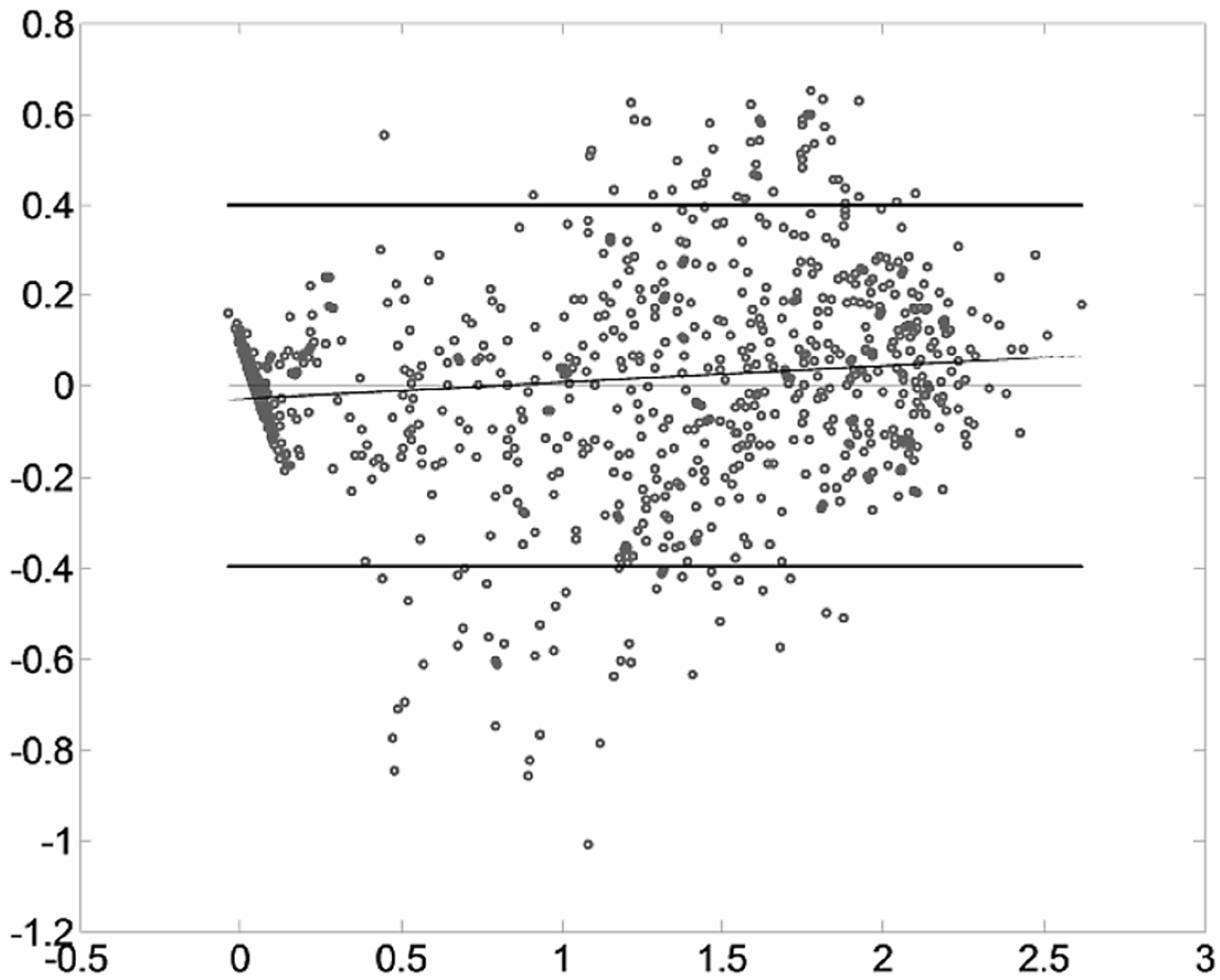
2.3. Bland-Altman Plots

Bland-Altman’s analysis and plot are among the most common methods used to assess the relative agreement between two analytical methods. By showing the difference between two estimates versus their mean, three important features of the methods comparison can be determined by visual inspection:

• The 1.96 σ_diff boundary for the difference distribution, pointing out how much the two methods spread.
• The regularity of the distribution along the mean axis, to identify variable-related error patterns.
• The symmetry of the distribution around the zero, addressing systematic bias of the measurements.

Bland-Altman plots can be used to know by how much the new method is likely to differ from the old: if this is not enough to cause problems in results interpretation, it is possible to replace the old method by the new or use the two interchangeably [32,42].

2.4. Experimental Protocol and Validation

A previously acquired set of data was used to validate the approach proposed in this paper. These data were obtained by pedaling on a cycling simulator for sessions about 50 minutes long with a pedaling cadence fixed at 70 rounds per minute (rpm). The cycling simulator was equipped with a system to control the power exerted by the participant [43,44]. This system has been validated in recent works as suitable for force and power measuring during cycling activity in real time [45]. Force data, obtained from the previous work [15], were acquired (2000 Samples/s sampling frequency, 12-bit A/D converter) by a homemade instrumented pedal mounted on the cycling simulator. With this system, it was possible to measure force components exerted on the pedal, the angular displacement of the pedal, θ_P, and the angular displacement of the crank, θ_C. These data were used as input for the biomechanical model described above. The experimental protocol was used for the estimation of the muscular forces using the two different techniques and its validation was:

• Training and validation set of NNs using data obtained previously by a deterministic optimization algorithm.
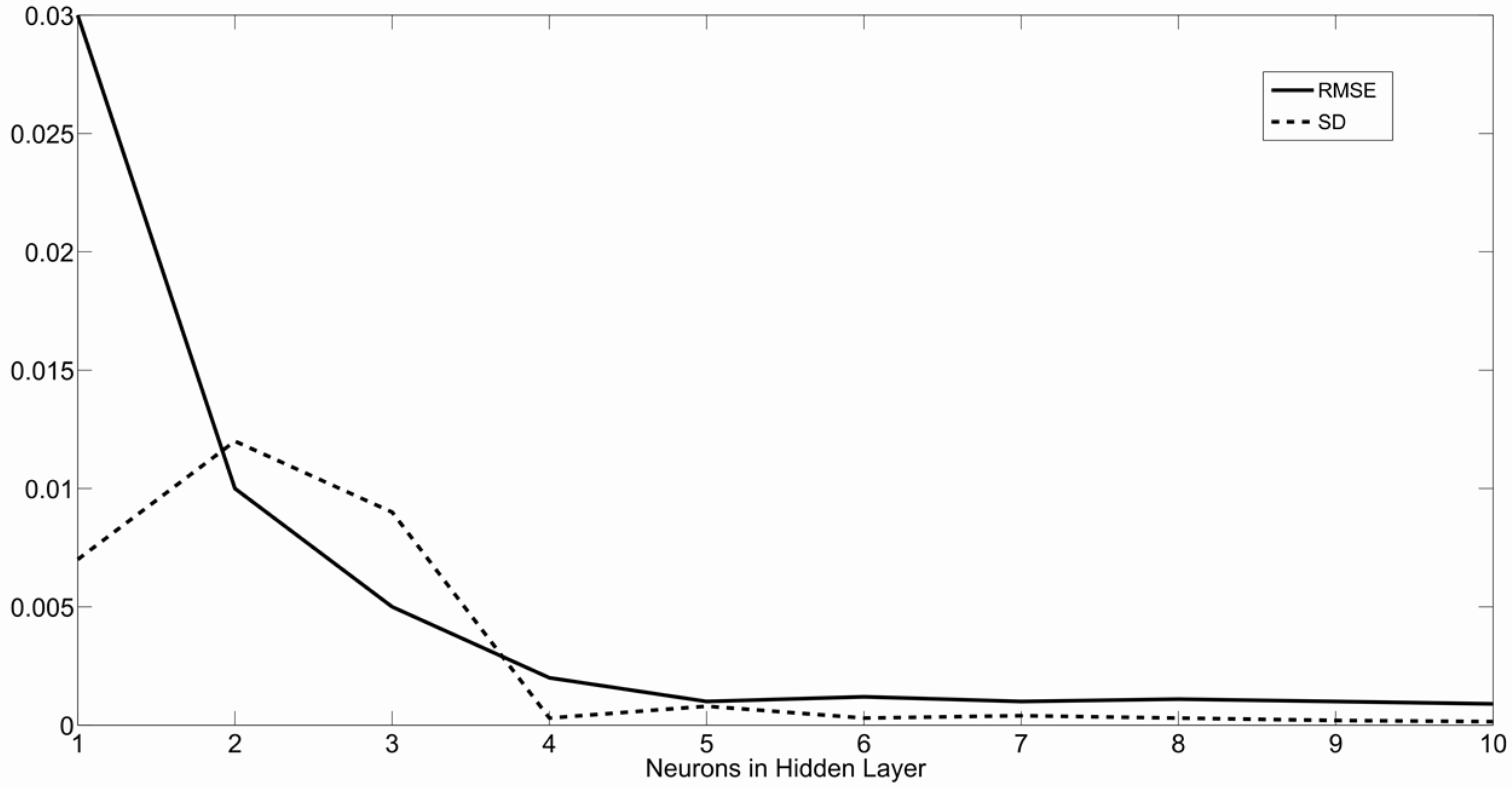
• Plot analysis between the signals obtained by NNs and signals obtained by the optimization algorithm, and the evaluation of the RMSE and RMSE Standard Deviation.
• Validation of the experimental protocol analyzing Bland-Altman plots extrapolating 1180 random samples from each muscle forces signals.

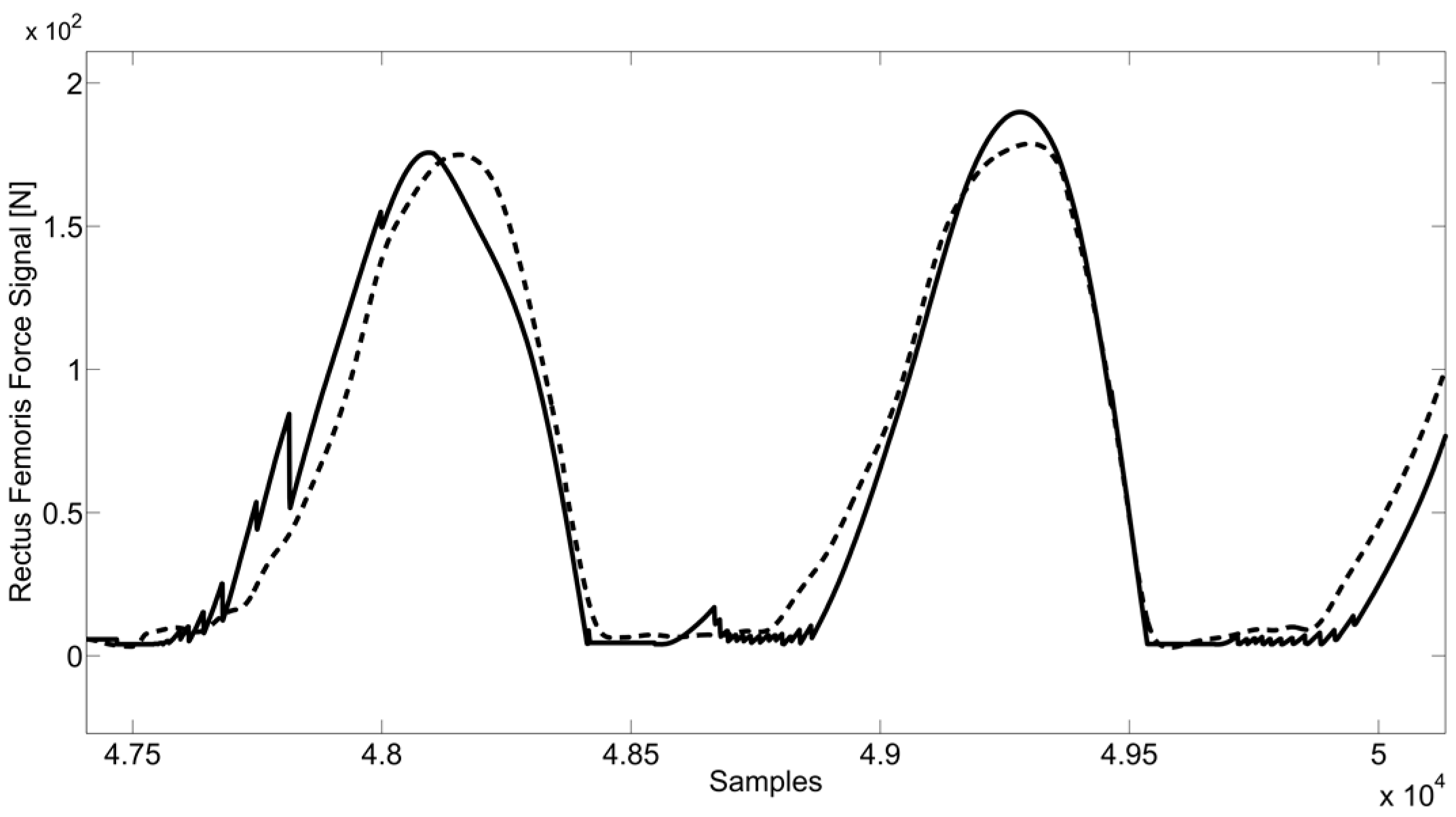
3. Results and Discussion

In this section, all obtained results are displayed and discussed. To obtain the results, two NN were implemented on the basis of the parameters reported in the following Table 1: the first NN was used to calculate the angle θ_s (θ_c, θ_p) solving a non linear equation, while the second one was used to estimate muscular forces optimizing the cost function described above.

Table 1. Parameters of Neural Networks (NN) used to obtain the results.

Output	NN topology	Number of inputs	Number of neurons in the hidden layer	Training set (Samples)	Validation set (Samples)
θS angle	1 MISO	2	4	7,050	118,000
Muscle Forces	9 MISO	3	15	2,360	118,000

Table 1. Parameters of Neural Networks (NN) used to obtain the results.

Output	NN topology	Number of inputs	Number of neurons in the hidden layer	Training set (Samples)	Validation set (Samples)
θS angle	1 MISO	2	4	7,050	118,000
Muscle Forces	9 MISO	3	15	2,360	118,000

The θ_S angle estimated signals, for one of the subject, obtained using deterministic algorithm optimization and using neural network are both shown in Figure 5.

Figure 5. Angle θ_S signals, obtained by the deterministic optimization algorithm (solid gray) and by the neural network (dashed black).

Figure 5. Angle θ_S signals, obtained by the deterministic optimization algorithm (solid gray) and by the neural network (dashed black).

In the Table 2 the correlation of the two signals, for three different subjects, is shown in terms of Root Mean Square Error (RMSE).

Table 2. Results of RMS Error percentage and SD Error for the calculation of θ_S angle.

Subject	RMS Error %	Standard Deviation Error
1	0.085%	2.68 × 10−4
2	0.134%	7.35 × 10−4
3	0.077%	4.53 × 10−4

Table 2. Results of RMS Error percentage and SD Error for the calculation of θ_S angle.

Subject	RMS Error %	Standard Deviation Error
1	0.085%	2.68 × 10−4
2	0.134%	7.35 × 10−4
3	0.077%	4.53 × 10−4

Neural network, for all three subjects, makes a RMS Error well below 1% and a SD Error below 10⁻³, showing a good convergence in the research of the optimal solution.

Regarding the second step, 1180 random samples out of 118,000 have been taken for the analysis of the results. In the Figure 6, the Bland-Altman plot for the Rectus Femoris is shown.

While the 1.96 σ_diff boundaries are not negligibly narrow, they can be reasonably attributed to the intrinsic noise affecting the deterministic algorithm (more on this matter will be discussed below). The distribution is acceptably symmetric around the mean axis, excluding the possibility of a systematic measurement error. There is no apparent pattern in the error distribution apart from a border effect, consisting in a clustering of samples on the left side around the axis origin. This is due to boundary conditions used in the model: muscular forces cannot have negative value, because of obvious physiological reasons. In Table 3, both the upper and lower 1.96_σdiff boundaries are shown, together with the width of the boundary divided by the relative muscle mean force (normalized boundary).

Figure 6. Bland-Altman Results for the rectus femoris muscle.

Figure 6. Bland-Altman Results for the rectus femoris muscle.

Table 3. Upper, lower and normalized boundaries for the nine muscle forces.

Muscle	Upper Boundary	Lower Boundary	Normalized Boundary
TA	0.1573	−0.1577	0.6707
SO	0.6296	−0.6341	0.0786
GA	0.5829	−0.5845	0.4660
VA	0.1203	−0.1212	0.0794
RF	0.3996	−0.3967	0.4155
BFs	0.08088	−0.08076	0.6616
BFl	0.7286	−0.7266	0.1354
IL	0.2739	−0.2748	0.1873
GLM	0.9368	−0.9251	0.1311

Table 3. Upper, lower and normalized boundaries for the nine muscle forces.

Muscle	Upper Boundary	Lower Boundary	Normalized Boundary
TA	0.1573	−0.1577	0.6707
SO	0.6296	−0.6341	0.0786
GA	0.5829	−0.5845	0.4660
VA	0.1203	−0.1212	0.0794
RF	0.3996	−0.3967	0.4155
BFs	0.08088	−0.08076	0.6616
BFl	0.7286	−0.7266	0.1354
IL	0.2739	−0.2748	0.1873
GLM	0.9368	−0.9251	0.1311

Aside from the error, a consideration can be made on the networks performance predicting muscular forces. Indeed, the number of unknowns in (2) is higher than the number of equations (9 unknowns for 3 equations), so the numerical optimization of such problem is multimodal, yielding a very noisy solution. The NN however performs an average of the different solutions, smoothing effectively the results. This effect is highlighted in Figure 7: the NN completely filters unnatural “high” frequency components in the muscular activity signals.

In terms of computational complexity, the computational time required to elaborate a full sample, thus to compute the nine muscular forces starting from the pedals data, is about 26 ms on a Core i7 Machine, against the 2,200 ms required to compute the deterministic original approach on the same machine, yielding a considerable speed up.

Figure 7. Muscle forces of rectus femoris obtained with the neural network (dashed) and with the deterministic algorithm optimization (solid). Sampling frequency 1000 Samples/s.

Figure 7. Muscle forces of rectus femoris obtained with the neural network (dashed) and with the deterministic algorithm optimization (solid). Sampling frequency 1000 Samples/s.

4. Conclusions and Future Developments

In this paper, an optimized alternative approach to estimate muscle force patterns of an athlete during cycling activity using NNs has been presented. The NNs were trained using the results obtained with a validated method that uses a deterministic optimization algorithm. The validation of the estimation obtained by NNs was accomplished analyzing the Bland-Altman plot, used to evaluate agreement between the two different methods. The results have been compared showing a good agreement between the two methods and the neural network was able to display smoother signals, as compared to the deterministic optimization. A further result can be appreciated in the significantly reduced computational costs provided by the use of NNs. Indeed, whereas the optimization algorithm requires an iterative evaluation of several non-linear functions, the NN can be evaluated directly in much less time. The considerable reduction in computational time (as shown in section 3, about two orders of magnitude as compared to the previous method) opens the possibility of implementing this approach in embedded environment using low level language. Moreover, the sampling frequency adopted in this work (i.e. 1000 Samples/s) was higher than necessary and used only in accord with the previous work [15]. In a future real time application the sampling frequency necessary to acquire forces and angles data can be reduced down to 30 Samples/s. This value is compatible with the lower computational cost found for the NNs approach, as shown in the results. Of course, the use of this approach is, as of now, subject specific: since the Neural Network requires to be trained on a specific dataset, the original deterministic algorithm must run at least once. However, this operation can be performed off-line and just one time. Once the neural networks are trained, the prediction can be performed at full speed with the method proposed in this work. On the Neural Network specific performance, even if the results for the prediction were satisfactory, an increase in the variance of the anthropometric characteristics subjects could be desired. Indeed, the generalization capabilities of the network are inherently tied to the variance of the training pattern, and to ensure the usability of this neural system for a variety of participants, a larger population should be used. The enlargement of the sample size, however, can yield a more complex optimization problem, which could require parallel architectures and advanced algorithms to be solved [46,47,48,49].

References

1. Erdemir, A.; McLean, S.; Herzog, W.; van den Bogert, A.J. Model-based estimation of muscle forces exerted during movements. Clin. Biomech. 2007, 22, 131–154. [Google Scholar] [CrossRef] [PubMed]
2. Pandy, M.G.; Andriacchi, T.P. Muscle and joint function in human locomotion. Annu. Rev. Biomed. Eng. 2010, 12, 401–433. [Google Scholar] [CrossRef] [PubMed]
3. Hughes, R.E.; An, K.N. Monte Carlo simulation of a planar shoulder model. Med. Biol. Eng. Comput. 1997, 35, 544–548. [Google Scholar] [CrossRef] [PubMed]
4. Dorn, T.W.; Schache, A.G.; Pandy, M.G. Muscular strategy shift in human running: Dependence of running speed on hip and ankle muscle performance. J. Exp. Biol. 2012, 25, 1944–1956. [Google Scholar] [CrossRef] [PubMed]
5. Ingram, D.; Müllhaupt, P.; Terrier, A.; Farron, A. Dynamical Biomechanical Model of the Shoulder for Muscle-Force Estimation. In Proceedings of 4th IEEE RAS/EMBS International Conference on Biomedical Robotics and Biomechatronics, Rome, Italy, 24–27 June 2012.
6. Aeberhard, M.; Michellod, Y.; Mullhaupt, P.; Terrier, A.; Pioletti, D.P.; Gillet, D. Dynamical Biomechanical Model of the Shoulder: Null Space Based Optimization of the Overactuated System. In Proceedings of Robotics and Biomimetics ROBIO 2008 IEEE International Conference, Bangkok, Thailand, 22–25 February 2009.
7. Terrier, A.; Aeberhard, M.; Michellod, Y.; Mullhaupt, P.; Pioletti, D.P.; Farron, A.; Gillet, D. A musculoskeletal shoulder model based on pseudo-inverse and null-spact5e optimization. Med. Eng. Phys. 2010, 32, 1050–1056. [Google Scholar] [CrossRef] [PubMed]
8. Mughal, A.M.; Kamran, I. 3D Bipedal Model for Biomechanical Sit-to-Stand Movement with Coupled Torque Optimization and Experimental Analysis. In Proceedings of Systems Man and Cybernetics (SMC) 2010 IEEE International Conference, Istanbul, Turkey, 10–13 October 2010.
9. Ferry, M.; Martin, L.; Termoz, N.; Côté, J.; Prince, F. Balance control during an arm raising movement in bipedal stance: Which biomechanical factor is controlled? Biol. Cybern. 2004, 91, 104–114. [Google Scholar] [CrossRef] [PubMed]
10. Castronovo, A.M.; Conforto, S.; Schmid, M.; Bibbo, D.; D’Alessio, T. How to assess performance in cycling: The multivariate nature of influencing factors and related indicators. Front. Physiol. 2013, 4, 116. [Google Scholar] [CrossRef] [PubMed]
11. Watson, M.; Bibbo, D.; Duffy, C.R.; Riches, P.E.; Conforto, S.; Macaluso, A. Validity and reliability of an alternative method for measuring power output during 6s all out cycling. J. Appl. Biomech. 2014, 30, 598–603. [Google Scholar] [CrossRef] [PubMed]
12. De Marchis, C.; Schmid, M.; Bibbo, D.; Castronovo, A.M.; D’Alessio, T.; Conforto, S. Feedback of mechanical effectiveness induces adaptations in motor modules during cycling. Front. Comput. Neurosci. 2013, 7, 1–12. [Google Scholar] [CrossRef] [PubMed]
13. De Marchis, C.; Schmid, M.; Bibbo, D.; Bernabucci, I.; Conforto, S. Inter-individual variability of forces and modular muscle coordination in cycling: A study on untrained subjects. Hum. Mov. Sci. 2013, 32, 1480–1494. [Google Scholar] [CrossRef] [PubMed]
14. De Marchis, C.; Castronovo, A.M.; Bibbo, D.; Schmid, M.; Conforto, S. Muscle Synergies are Consistent when Pedaling under Different Biomechanical Demands. In Proceedings of the 34th IEEE-EMBS Conference, San Diego, CA, USA, 28 August–1 September 2012; Volume 1, pp. 3308–3311.
15. Bibbo, D.; Conforto, S.; Gallozzi, C.; D’Alessio, T. Combining electrical and mechanical data to evaluate muscular activities during cycling. WSEAS Trans. Biol. Biomed. 2006, 5, 339–346. [Google Scholar]
16. Prilutsky, B.I. Coordination of two-and one-joint muscles: Functional consequences and implications for motor control. Mot. Control 2000, 4, 1–44. [Google Scholar]
17. Prilutsky, B.I.; Zatsiorsky, V.M. Optimization-based models of muscle coordination. Exerc. Sp. Sci. Rev. 2002, 30, 32. [Google Scholar] [CrossRef]
18. Bottasso, C.L.; Prilutsky, B.I.; Croce, A.; Imberti, E.; Sartirana, S. A numerical procedure for inferring from experimental data the optimization cost functions using a multibody model of the neuro-musculoskeletal system. Multibody Syst. Dyn. 2006, 16, 123–154. [Google Scholar] [CrossRef]
19. D’Alessio, T.; Conforto, S. Extraction of the envelope from surface EMG signals: An adaptive procedure for dynamic protocols. IEEE Eng. Med. Biol. Mag. 2001, 6, 55–61. [Google Scholar] [CrossRef]
20. Conforto, S.; D’Alessio, T.; Pignatelli, S. Optimal rejection of movement artefacts from myoelectric signals by means of a wavelet filtering procedure. J. Electromyogr. Kinesiol. 1999, 9, 47–57. [Google Scholar] [CrossRef]
21. Hornik, K.; Stinchcombe, M.; White, H. Multilayer feedforward networks are universal approximators. Neural Netw. 1989, 2, 359–366. [Google Scholar] [CrossRef]
22. Chen, T.P.; Chen, H. Universal approximation to nonlinear operators by neural networks with arbitrary activation functions and its application to dynamical systems. IEEE Trans. Neural Netw. 1995, 6, 911–917. [Google Scholar] [CrossRef] [PubMed]
23. Leshno, M.; Lin, V.Y.; Pinkus, A.; Schocken, S. Multilayer feedforward networks with a nonpolynomial activation function can approximate any function. Neural Netw. 1993, 6, 861–867. [Google Scholar] [CrossRef]
24. Chen, T.P.; Chen, H. Approximations of continuous functional by neural networks with application to dynamic systems. IEEE Trans. Neural Netw. 1993, 4, 910–918. [Google Scholar] [CrossRef] [PubMed]
25. Chen, T.P.; Chen, H.; Liu, R.W. Approximation capability in C (Rn) by multilayer feedforward networks and related problems. IEEE Trans. Neural Netw. 1995, 6, 25–30. [Google Scholar] [CrossRef] [PubMed]
26. Tamura, S.; Tateishi, M. Capabilities of a four-layered feedforward neural network: Four layers versus three. IEEE Trans. Neural Netw. 1997, 8, 251–255. [Google Scholar] [CrossRef] [PubMed]
27. De Villiers, J.; Barnard, E. Backpropagation neural nets with one and two hidden layers. IEEE Trans. Neural Netw. 1993, 4, 136–141. [Google Scholar] [CrossRef] [PubMed]
28. Razavi, S.; Tolosn, B.A.; Burn, D.H. Numerical assessment of metamodelling strategies in computationally intensive optimization. Environ. Modell Softw. 2011, 34, 67–86. [Google Scholar] [CrossRef]
29. Bishop, C.M. Neural Networks for Pattern Recognition; Oxford University Press: Oxford, UK, 1995. [Google Scholar]
30. Krejcar, O.; Penhaker, M.; Janckulik, D.; Motalova, L. Performance Test of Multiplatform Real Time Processing of Biomedical Signals. In Proceedings of 8th IEEE International Conference on Industrial Informatics, Osaka, Japan, 13–16 July 2010.
31. Van den Bogert, A.J.; Geijtenbeek, T.; Even-Zohar, O.; Steenbrink, F.; Hardin, E.C. A real-time system for biomechanical analysis of human movement and muscle function. Med. Biol. Eng. Comput. 2013, 51, 1069–1077. [Google Scholar] [CrossRef] [PubMed]
32. Bland, M.J.; Altman, D. Statistical methods for assessing agreement between two methods of clinical measurement. Lancet 1986, 327, 307–310. [Google Scholar] [CrossRef]
33. Lam, A.; Chen, D.; Chiu, R.; Chui, W.S. Comparison of IOP measurements between ORA and GAT in normal Chinese. Optom. Vis. Sci. 2007, 84, 909–914. [Google Scholar] [CrossRef] [PubMed]
34. De Leva, P. Adjustments to Zatsiorsky-Seluyanov’s segment inertia parameters. J Biomech. 1996, 29, 1223–1230. [Google Scholar] [CrossRef]
35. Prilutsky, B.I.; Gregor, R.J. Strategy of coordination of two- and one-joint leg muscles in controlling an external force. Mot. Control 1997, 1, 92–116. [Google Scholar]
36. Crowninshield, R.D.; Brand, R.A. A physiologically based criterion of muscle force prediction in locomotion. J. Biomech. 1981, 14, 793–801. [Google Scholar] [CrossRef]
37. Dul, J.; Johnson, J.E.; Schiavi, R.; Townsend, M.A. Muscular synergism—II. A minimum-fatigue criterion for load sharing between synergistic muscles. J. Biomech. 1984, 17, 675–684. [Google Scholar]
38. Hagan, M.T.; Menhaj, M.B. Training feed forward networks with the Marquardt algorithm. IEEE Trans. Neural Netw. 1994, 5, 989–993. [Google Scholar] [CrossRef] [PubMed]
39. Beale, M.H.; Hagan, M.T.; Demuth, H.B. Neural Network Toolbox 7. Available online: http://www.mathworks.cn/products/techkitpdfs/8511.pdf (accessed on 15 August 2014).
40. Capizzi, G.; Coco, S.; Giuffrida, C.; Laudani, A. A neural network approach for the differentiation of numerical solutions of 3-D electromagnetic problems. IEEE Trans. Magn. 2004, 2, 953–956. [Google Scholar] [CrossRef]
41. Fulginei, F.R.; Salvini, A.; Parodi, A.M. Learning optimization of neural networks used for MIMO applications based on multivariate functions decomposition. Inverse Probl. Sci. Eng. 2012, 20, 29–39. [Google Scholar] [CrossRef]
42. Bland, M.J.; Altman, D. Validating scales and indexes. BMJ Br. Med. J. 2002, 324, 606. [Google Scholar] [CrossRef]
43. Bibbo, D.; Conforto, S.; Schmid, M.; D’Alessio, T. A Wireless Integrated System to Evaluate Efficiency Indexes in Real Time during Cycling. In Proceedings of the 4th European Conference of the International Federation for Medical and Biological Engineering IFMBE Proceedings, Antwerp, Belgium, 23–27 November 2008; Volume 22, pp. 89–92.
44. Conforto, S.; Sciuto, S.A.; Bibbo, D.; Scorza, A. Calibration of a Measurement System for the Evaluation of Efficiency Indexes in Bicycle Training. In Proceedings of the 4th European Conference of the International Federation for Medical and Biological Engineering IFMBE Proceedings, Antwerp, Belgium, 23–27 November 2008; Volume 22, pp. 106–109.
45. Bibbo, D.; Conforto, S.; Bernabucci, I.; Carli, M.; Schmid, M.; D’Alessio, T. Analysis of Different Image-Based Biofeedback Models for Improving Cycling Performances. In Proceedings of SPIE 2012 the International Society for Optical Engineering, San Francisco, CA, USA, 9–10 January 2012; p. 829503.
46. Fulginei, F.R.; Salvini, A.; Pulcini, G. Metric-topological-evolutionary optimization. Inverse Probl. Sci. Eng. 2012, 20, 41–58. [Google Scholar] [CrossRef]
47. Coco, S.; Laudani, A.; Pulcini, G.; Fulginei, F.R.; Salvini, A. Shape optimization of multistage depressed collectors by parallel evolutionary algorithm. IEEE Trans. Magn. 2012, 48, 435–438. [Google Scholar] [CrossRef]
48. Laudani, A.; Fulginei, F.R.; Lozito, G.M.; Salvini, A. Swarm/flock optimization algorithms as continuous dynamic systems. Appl. Math. Comput. 2014, 243, 670–683. [Google Scholar] [CrossRef]
49. Laudani, A.; Fulginei, F.R.; Salvini, A.; Schmid, M.; Conforto, S. CFSO3: A new supervised swarm-based optimization algorithm. Math. Probl. Eng. 2013, 2013, 560614. [Google Scholar] [CrossRef]