
On String Matching with Mismatches

Department of Computer Science and Engineering, University of Connecticut, 371 Fairfield Way Unit 4155, Storrs, CT 06269, USA
*
Author to whom correspondence should be addressed.
Algorithms 2015, 8(2), 248-270; https://0-doi-org.brum.beds.ac.uk/10.3390/a8020248
Submission received: 3 April 2015
/
Accepted: 19 May 2015
/
Published: 26 May 2015
(This article belongs to the Special Issue Algorithmic Themes in Bioinformatics)
Abstract
:In this paper, we consider several variants of the pattern matching with mismatches problem. In particular, given a text and a pattern , we investigate the following problems: (1) pattern matching with mismatches: for every output, the distance between P and ; and (2) pattern matching with k mismatches: output those positions i where the distance between P and is less than a given threshold k. The distance metric used is the Hamming distance. We present some novel algorithms and techniques for solving these problems. We offer deterministic, randomized and approximation algorithms. We consider variants of these problems where there could be wild cards in either the text or the pattern or both. We also present an experimental evaluation of these algorithms. The source code is available at http://www.engr.uconn.edu/∼man09004/kmis.zip.
1. Introduction
The problem of string matching has been studied extensively due to its wide range of applications from Internet searches to computational biology. String matching can be defined as follows. Given a text and a pattern , with letters from an alphabet Σ, find all of the occurrences of the pattern in the text. This problem can be solved in time by using well-known algorithms (e.g., KMP[1]). A variation of this problem is to search for multiple patterns at the same time. An algorithm for this version is given in [2].
A more general formulation allows “don't care” or “wild card” characters in the text and the pattern. A wild card matches any character. An algorithm for pattern matching with wild cards is given in [3] and has a runtime of . The algorithm maps each character in Σ to a binary code of length . Then, a constant number of convolution operations is used to check for mismatches between the pattern and any position in the text. For the same problem, a randomized algorithm that runs in time with high probability is given in [4]. A slightly faster randomized algorithm is given in [5]. A simple deterministic time algorithm based on convolutions is given in [6].
A more challenging formulation of the problem is pattern matching with mismatches. This formulation appears in two versions: (1) for every alignment of the pattern in the text, find the distance between the pattern and the alignment; or (2) identify only those alignments where the distance between the pattern and the text is less than a given threshold. The distance metric can be the Hamming distance, edit distance, metric, and so on. The problem has been generalized to use trees instead of sequences or to use sets of characters instead of single characters (see [7]).
A survey of string matching with mismatches is given in [8]. A description of practical on-line string searching algorithms can be found in [9].
The Hamming distance between two strings A and B, of equal length, is defined as the number of positions where the two strings differ and is denoted by .
In this paper, we are interested in the following two problems, with and without wild cards.
1. Pattern matching with mismatches: Given a text and a pattern , output , for every .
2. Pattern matching with k mismatches (or the k mismatches problem): Take the same input as above, plus an integer k. Output all i, , for which .
1.1. Pattern Matching with Mismatches
For pattern matching with mismatches, a naive algorithm computes the Hamming distance for every alignment of the pattern in the text, in time . A faster algorithm, in the absence of wild cards, is Abrahamson's algorithm [10] that runs in time. Abrahamson's algorithm can be extended to solve pattern matching with mismatches and wild cards, as we prove in Section 2.2.1. The new algorithm runs in time, where g is the number of non-wild card positions in the pattern. This gives a simpler and faster alternative to an algorithm proposed in [11].
In the literature, we also find algorithms that approximate the number of mismatches for every alignment. For example, an approximate algorithm for pattern matching with mismatches, in the absence of wild cards, that runs in time, where r is the number of iterations of the algorithm, is given in [12]. Every distance reported has a variance bounded by where is the exact number of matches for alignment i.
Furthermore, a randomized algorithm that approximates the Hamming distance for every alignment within an ϵ factor and runs in time, in the absence of wild cards, is given in [13]. Here, c is a small constant. We extend this algorithm to pattern matching with mismatches and wild cards, in Section 2.3. The new algorithm approximates the Hamming distance for every alignment within an ϵ factor in time with high probability.
Recent work has also addressed the online version of pattern matching, where the text is received in a streaming model, one character at a time, and it cannot be stored in its entirety (see, e.g., [14,15,16]). Another version of this problem matches the pattern against multiple input streams (see, e.g., [17]). Another interesting problem is to sample a representative set of mismatches for every alignment (see, e.g., [18]).
1.2. Pattern Matching with K Mismatches
For the k mismatches problem, without wild cards, two algorithms that run in time are presented in [19,20]. A faster algorithm, that runs in time, is given in [11]. This algorithm combines the two main techniques known in the literature for pattern matching with mismatches: filtering and convolutions. We give a significantly simpler algorithm in Section 2.2.3, having the same worst case run time. The new algorithm will never perform more operations than the one in [11] during marking and convolution.
An intermediate problem is to check if the Hamming distance is less or equal to k for a subset of the aligned positions. This problem can be solved with the Kangaroo method proposed in [11] at a cost of time per alignment, using additional memory. We show how to achieve the same run time per alignment using only additional memory, in Section 2.2.2.
Further, we look at the version of k mismatches where wild cards are allowed in the text and the pattern. For this problem, two randomized algorithms are presented in [17]. The first one runs in time, and the second one in time. Both are Monte Carlo algorithms, i.e., they output the correct answer with high probability. The same paper also gives a deterministic algorithm with a run time of . Furthermore, a deterministic time algorithm is given in [21]. We present a Las Vegas algorithm (that always outputs the correct answer), in Section 2.4.3, which runs in time with high probability.
An algorithm for k mismatches with wild cards in either the text or the pattern (but not both) is given in [22]. This algorithm runs in time.
1.3. Our Results
The contributions of this paper can be summarized as follows.
For pattern matching with mismatches:
- An algorithm for pattern matching with mismatches and wild cards that runs in time, where g is the number of non-wild card positions in the pattern; see Section 2.2.1.
- A randomized algorithm that approximates the Hamming distance for every alignment, when wild cards are present, within an ϵ factor in time with high probability; see Section 2.3.
For pattern matching with k mismatches:
- An algorithm for pattern matching with k mismatches, without wild cards, that runs in time; this algorithm is simpler and has a better expected run time than the one in [11]; see Section 2.2.3.
- An algorithm that tests if the Hamming distance is less than k for a subset of the alignments, without wild cards, at a cost of time per alignment, using only additional memory; see Section 2.2.2.
- A Las Vegas algorithm for the k mismatches problem with wild cards that runs in time with high probability; see Section 2.4.3.
The rest of the paper is organized as follows. First, we introduce some notations and definitions. Then, we describe the exact, deterministic algorithms for pattern matching with mismatches and for k mismatches. Then, we present the randomized and approximate algorithms: first the algorithm for approximate counting of mismatches in the presence of wild cards, then the Las Vegas algorithm for k mismatches with wild cards. Finally, we present an empirical run time comparison of the deterministic algorithms and conclusions.
2. Materials and Methods
2.1. Some Definitions
Given two strings and (with ), the convolution of T and P is a sequence where , for . This convolution can be computed in time using the fast Fourier transform. If the convolutions are applied on binary inputs, as is often the case in pattern matching applications, some speedup techniques are presented in [23].
In the context of randomized algorithms, by high probability, we mean a probability greater or equal to where n is the input size and ϵ is a probability parameter usually assumed to be a constant greater than 0. The run time of a Las Vegas algorithm is said to be if the run time is no more than with probability greater or equal to for all , where c and are some constants and for any constant .
In the analysis of our algorithms, we will employ the following Chernoff bounds.
Chernoff bounds [24]: These bounds can be used to closely approximate the tail ends of abinomial distribution.
A Bernoulli trial has two outcomes, namely success and failure, the probability of success being p. A binomial distribution with parameters n and p, denoted as , is the number of successes in n independent Bernoulli trials.
Let X be a binomial random variable whose distribution is . If m is any integer , then the following are true:
for any .
2.2. Deterministic Algorithms
In this section, we present deterministic algorithms for pattern matching with mismatches. We start with a summary of two well-known techniques for counting matches: convolution and marking (see, e.g., [11]). In terms of notation, is the substring of T between i and j and stands for . Furthermore, the value at position i in array X is denoted by .
Convolution: Given a string S and a character α, define string , such that if , and 0 otherwise. Let . Then, gives the number of matches between P and where the matching character is α. Then, is the total number of matches between P and .
Marking: Given a character α, let be the set of positions where character α is found in P (i.e., ). Note that, if , then the alignment between P and will match , for all . This gives the marking algorithm: for every position i in the text, increment the number of matches for alignment , for all . In practice, we are interested in doing the marking only for certain characters, meaning we will do the incrementing only for the positions where . The algorithm then takes time. The pseudocode is given in Algorithm 1.
| Algorithm 1: |
 |
2.2.1. Pattern Matching with Mismatches
For pattern matching with mismatches, without wild cards, Abrahamson [10] gave the following time algorithm. Let A be a set of the most frequent characters in the pattern: (1) using convolutions, count how many matches each character in A contributes to every alignment; (2) using marking, count how many matches each character in contributes to every alignment; and (3) add the two numbers to find for every alignment, the number of matches between the pattern and the text. The convolutions take time. A character in cannot appear more than times in the pattern; otherwise, each character in A has a frequency greater than , which is not possible. Thus, the run time for marking is . If we equate the two run times, we find the optimal , which gives a total run time of .
An Example: Consider the case of and . Since each character in the pattern occurs an equal number of times, we can pick A arbitrarily. Let . In Step 1, convolution is used to count the number of matches contributed by each character in A. We obtain an array , such that is the number of matches contributed by characters in A to the alignment of P with , for . In this example, . In Step 2, we compute, using marking, the number of matches contributed by the characters 3 and 4 to each alignment between T and P. We get another array , such that is the number of matches contributed by 3 and 4 to the alignment between and P, for . Specific to this example, . In Step 3, we add and to get the number of matches between and P, for . In this example, this sum yields: .
For pattern matching with mismatches and wild cards, a fairly complex algorithm is given in [11]. The run time of this algorithm is where g is the number of non-wild card positions in the pattern. The problem can also be solved through a simple modification of Abrahamson's algorithm, in time , as pointed out in [17]. We now prove the following result:
Theorem 1.
Pattern matching with mismatches and wild cards can be solved in time, where g is the number of non-wild card positions in the pattern.
Proof.
Ignoring the wild cards for now, let A be the set of the most frequent characters in the pattern. As above, count matches contributed by characters in A and using convolution and marking, respectively. By a similar reasoning as above, the characters used in the marking phase will not appear more than times in the pattern. If we equate the run times for the two phases, we obtain time. We are now left to count how many matches are contributed by the wild cards. For a string S and a character α, define as . Let w be the wild card character. Compute . Then, for every alignment i, the number of positions that have a wild card either in the text, or the pattern, or both, is . Add to the previously-computed counts and output. The total run time is .
2.2.2. Pattern Matching with K Mismatches
For the k mismatches problem, without wild cards, an time algorithm that requires additional space is presented in [19]. Another algorithm, that takes time and uses only additional space, is presented in [20]. We define the following problem, which is of interest in the discussion.
Problem 1.
Subset k mismatches: Given a text T of length n, a pattern P of length m, a set of positions and an integer k, output the positions for which .
The subset k mismatches problem becomes the regular k mismatches problem if . Thus, it can be solved by the algorithms mentioned above. However, if , then the algorithms are too costly. A better alternative is to use the Kangaroo method proposed in [11]. The Kangaroo method can verify if in time for any i. The method works as follows. Build a suffix tree of and enhance it to support lowest common ancestor (LCA) queries. For a given i, perform an LCA query to find the position of the first mismatch between P and . Let this position be j. Then, perform another LCA to find the first mismatch between and , which is the second mismatch of alignment i. Continue to “jump” from one mismatch to the next, until the end of the pattern is reached or we have found more than k mismatches. The Kangaroo method can process positions in time, and it uses additional memory for the LCA enhanced suffix tree. We now prove the following result:
Theorem 2.
Subset k mismatches can be solved in time using only additional memory.
Proof.
The algorithm is the following. Build an LCA-enhanced suffix tree of the pattern. Scan the text from left to right: (1) find the longest unscanned region of the text that can be found somewhere in the pattern, say starting at position i of the pattern; call this region of the text R; therefore, R is identical to .; and (2) for every alignment in S that overlaps R, count the number of mismatches between R and the alignment, within the overlap region. To do this, consider an alignment in S that overlaps R, such that the beginning of R aligns with the j-th character in the pattern. We want to count the number of mismatches between R and . However, since R is identical to , we can simply compare and . This comparison can be done efficiently by jumping from one mismatch to the next, like in the Kangaroo method. Repeat from Step 1 until the entire text has been scanned. Every time we process an alignment, in Step 2, we either discover at least one additional mismatch or we reach the end of the alignment. This is true, because, otherwise, the alignment would match the text for more than characters, which is not possible, from the way we defined R. Every alignment for which we have found more than k mismatches is excluded from further consideration to ensure time per alignment. It takes time to build the LCA enhanced suffix tree of the pattern and additional time to scan the text from left to right. Thus, the total run time is with additional memory. The pseudocode is given in Algorithm 2.
2.2.3. An Time Algorithm for K Mismatches
For the k mismatches problem, without wild cards, a fairly complex time algorithm is given in [11]. The algorithm classifies the inputs into several cases. For each case, it applies a combination of marking followed by a filtering step, the Kangaroo method, or convolutions. The goal is to not exceed time in any of the cases. We now present an algorithm with only two cases that has the same worst case run time. The new algorithm can be thought of as a generalization of the algorithm in [11], as we will discuss later. This generalization not only greatly simplifies the algorithm, but it also reduces the expected run time. This happens because we use information about the frequency of the characters in the text and try to minimize the work done by convolutions and marking.
| Algorithm 2: Subset k mismatches() |
 |
We will now give the intuition for this algorithm. For any character , let be its frequency in the pattern and be its frequency in the text. Note that in the marking algorithm, a specific character α will contribute to the runtime a cost of . On the other hand, in the case of convolution, a character α costs us one convolution, regardless of how frequent α is in the text or the pattern. Therefore, we want to use infrequent characters for marking and frequent characters for convolution. The balancing of the two will give us the desired runtime.
A position j in the pattern where is called an instance of α. Consider every instance of character α as an object of size 1 and cost . We want to fill a knapsack of size at a minimum cost and without exceeding a given budget B. The instances will allow us to filter some of the alignments with more than k mismatches, as will become clear later. This problem can be optimally solved by a greedy approach, where we include in the knapsack all of the instances of the least expensive character, then all of the instances of the second least expensive character, and so on, until we have items or we have exceeded B. The last character considered may have only a subset of its instances included, but for the ease of explanation, assume that there are no such characters.
Note: Even though the above is described as a knapsack problem, the particular formulation can be optimally solved in linear time. This formulation should not be confused with other formulations of the knapsack problem that are NP-complete.
Case (1): Assume we can fill the knapsack at a cost . We apply the marking algorithm for the characters whose instances are included in the knapsack. It is easy to see that the marking takes time and creates C marks. For alignment i, if the pattern and the text match for all of the positions in the knapsack, we will obtain exactly marks at position i. Conversely, any position that has less than k marks must have more than k mismatches, so we can filter it out. Therefore, there will be at most positions with k marks or more. For such positions, we run subset k mismatches to confirm which of them have less than k mismatches. The total runtime of the algorithm in this case is .
Case (2): If we cannot fill the knapsack within the given budget B, we do the following: for the characters we could fit in the knapsack, we use the marking algorithm to count the number of matches that they contribute to each alignment. For characters not in the knapsack, we use convolutions to count the number of matches that they contribute to each alignment. We add the two counts and get the exact number of matches for every alignment.
Note that at least one of the instances in the knapsack has a cost larger than (if all of the instances in the knapsack had a cost less or equal to , then we would have at least instances in the knapsack). Furthermore, note that all of the instances not in the knapsack have a cost at least as high as any instance in the knapsack, because we greedily fill the knapsack starting with the least costly instances. This means that every character not in the knapsack appears in the text at least times. This means that the number of characters not in the knapsack does not exceed . Therefore, the total cost of convolutions is . Since the cost of marking was , we can see that the best value of B is the one that equalizes the two costs. This gives . Therefore, the algorithm takes time. If , we can employ a different algorithm that solves the problem in linear time, as in [11]. For larger k, , so the run time becomes . We call this algorithm knapsack k mismatches. The pseudocode is given in Algorithm 3. The following theorem results.
Theorem 3.
Knapsack k mismatches has worst case run time .
| Algorithm 3: Knapsack k mismatches() |
 |
We can think of the algorithm in [11] as a special case of our algorithm where, instead of trying to minimize the cost of the items in the knapsack, we just try to find items for which the cost is less than . As a result, it is easy to verify the following:
Theorem 4.
Knapsack k mismatches spends at most as much time as the algorithm in [11] to do convolutions and marking.
Proof.
Observation: In all of the cases presented below, knapsack k mismatches can have a run time as low as , for example if there exists one character α with and .
Case 1: . The algorithm in [11] chooses instances of distinct characters to perform marking. Therefore, for every position of the text, at most one mark is created. If the number of marks is M, then the cost of the marking phase is . The number of remaining positions after filtering is no more than , and thus, the algorithm takes time. Our algorithm puts in the knapsack 2k instances, of not necessarily different characters, such that the number of marks B is minimized!Therefore, , and the total runtime is .
Case 2: . The algorithm in [11] performs one convolution per character to count the total number of matches for every alignment, for a run time of . In the worst case, knapsack k mismatches cannot fill the knapsack at a cost , so it defaults to the same run time. However, in the best case, the knapsack can be filled at a cost B as low as depending on the frequency of the characters in the pattern and the text. In this case, the runtime will be .
Case 3: . A symbol that appears in the pattern at least times is called frequent.
Case 3.1: There are at least frequent symbols. The algorithm in [11] chooses instances of frequent symbols to do marking and filtering at a cost . Since knapsack k mismatches will minimize the marking time B, we have , so the run time is the same as for [11] only in the worst case.
Case 3.2: There are frequent symbols. The algorithm in [11] first performs one convolution for each frequent character for a run time of . Two cases remain:
Case 3.2.1: All of the instances of the non-frequent symbols number less than positions. The algorithm in [11] replaces all instances of frequent characters with wild cards and applies a algorithm to count mismatches, where g is the number of non-wild card positions. Since , the run time for this stage is , and the total run time is . Knapsack k mismatches can always include in the knapsack all of the instances of non-frequent symbols, since their total cost is no more than , and in the worst case, do convolutions for the remaining characters. The total run time is . Of course, depending on the frequency of the characters in the pattern and text, knapsack k mismatch may not have to do any convolutions.
Case 3.2.2: All of the instances of the non-frequent symbols number at least positions. The algorithm in [11] chooses instances of infrequent characters to do marking. Since each character has a frequency less than , the time for marking is , and there are no more than positions left after filtering. Knapsack k mismatches chooses characters in order to minimize the time B for marking, so again .
2.3. Approximate Counting of Mismatches
The algorithm of [13] takes as input a text and a pattern and approximately counts the Hamming distance between and P for every . In particular, if the Hamming distance between and P is for some i, then the algorithm outputs where for any with high probability (i.e., a probability of . The run time of the algorithm is . In this section, we show how to extend this algorithm to the case where there could be wild cards in the text and/or the pattern.
Let Σ be the alphabet under concern, and let . The algorithm runs in phases, and in each phase, we randomly map the elements of Σ to . A wild card is mapped to a zero. Under this mapping, we transform T and P to and , respectively. We then compute a vector C where . This can be done using convolution operations (as in Section 2.4.1; see also [17]). A series of r such phases (for some relevant value of r) is done, at the end of which, we produce estimates on the Hamming distances. The intuition is that if a character x in is aligned with a character y in , then across all of the r phases, the expected contribution to C from these characters is r if (assuming that x and y are non-wild cards). If or if one or both of x and y are a wild card, the contribution to C is zero.
| Algorithm 4: |
 |
Analysis: Let x be a character in T, and let y be a character in P. Clearly, if or if one or both of x and y are a wild card, the contribution of x and y to any is zero. If x and y are non-wild cards and if , then the expected contribution of these to any is 1. Across all of the r phases, the expected contribution of x and y to any is r. For a given x and y, we can think of each phase as a Bernoulli trial with equal probabilities for success and failure. A success refers to the possibility of . The expected number of successes in r phases is . Using Chernoff bounds (Equation 2), this contribution is no more than with probability . The probability that this statement holds for every pair is . This probability will be if . Similarly, we can show that for any pair of non-wild card characters, the contribution of them to any is no less than with probability if .
Put together, for any pair of non-wild cards, the contribution of x and y to any is in the interval with probability if . Let be the Hamming distance between and P for some i (. Then, the estimate on will be in the interval with probability . As a result, we get the following Theorem.
Theorem 5.
Given a text T and a pattern P, we can estimate the Hamming distance between and P, for every , in time. If is the Hamming distance between and P, then the above algorithm outputs an estimate that is in the interval with high probability.
Observation 1. In the above algorithm, we can ensure that and with high probability by changing the estimate computed in Step 3 of Algorithm 4 to .
Observation 2. As in [13], with pre-processing, we can ensure that Algorithm 4 never errs (i.e., the error bounds on the estimates will always hold).
2.4. A Las Vegas Algorithm for K Mismatches
2.4.1. The 1 Mismatch Problem
Problem definition: For this problem, also, the inputs are two strings T and P with and possible wild cards in T and P. Let stand for the substring , for any i, with . The problem is to check if the Hamming distance between and P is exactly 1, for . The following Lemma is shown in [17].
Lemma 1.
The 1 mismatch problem can be solved in time using a constant number of convolution operations.
The algorithm: Assume that each wild card in the pattern as well as the text is replaced with a zero. Furthermore, assume that the characters in the text, as well as the pattern are integers in the range where Σ is the alphabet of concern. Let stand for the “error term” introduced by the character in and the character in P, and its value is . Furthermore, let . There are four steps in the algorithm:
- Compute for . Note that will be zero if and P match (assuming that a wild card can be matched with any character). . Thus, this step can be completed with three convolution operations.
- Compute for , where (for . Like Step 1, this step can also be completed with three convolution operations.
- Let if , for . Note that if the Hamming distance between and P is exactly one, then will give the position in the text where this mismatch occurs.
- If for any i (), and if , then we conclude that the Hamming distance between and P is exactly one.
Note: If the Hamming distance between and P is exactly 1 (for any i), then the above algorithm will not only detect it, but also will identify the position where there is a mismatch. Specifically, it will identify the integer j, such that .
An example. Consider the case where and . Here, * represents the wild card.
In Step 1, we compute , for 1 . For example, ; ; ; . Note that since is a wild card, it matches with any character in the pattern. Furthermore, .
In Step 2, we compute , for . For instance, ; .
In Step 3, the value of is computed for . For example, ; .
In Step 4, we identify all of the positions in the text corresponding to a single mismatch. For instance, we note that and . As a result, Position 5 in the text correspondsto 1 mismatch.
2.4.2. The Randomized Algorithms of [17]
Two different randomized algorithms are presented in [17] for solving the k mismatches problem. Both are Monte Carlo algorithms. In particular, they output the correct answers with high probability. The run times of these algorithms are and , respectively. In this section, we provide a summary of these algorithms.
The first algorithm has sampling phases, and in each phase, a 1 mismatch problem is solved. Each phase of sampling works as follows. We choose positions of the pattern uniformly at random. The pattern P is replaced by a string where , the characters in in the randomly chosen positions are the same as those in the corresponding positions of P, and the rest of the characters in are set to wild cards. The 1 mismatch algorithm of Lemma 1 is run on T and . In each phase of random sampling, for each i, we get to know if the Hamming distance between and is exactly 1, and, if so, identify the j, such that .
As an example, consider the case when the Hamming distance between and P is k (for some i). Then, in each phase of sampling, we would expect to identify exactly one of the positions (i.e., j) where and P differ (i.e., ). As a result, in an expected k phases of sampling, we will be able to identify all of the k positions in which and P differ. It can be shown that if we make sampling phases, then we can identify all of the k mismatches with high probability [17]. It is possible that the same j might be identified in multiple phases. However, we can easily keep track of this information to identify the unique j values found in all of the phases.
Let the number of mismatches between and P be (for . If , the algorithm of [17] will compute exactly. If , then the algorithm will report that the number of mismatches is (without estimating ), and this answer will be correct with high probability. The algorithm starts off by first computing values for every . A list of all of the mismatches found for is kept, for every i. Whenever a mismatch is found between and P (say in position of the text), the value of is reduced by . If at any point in the algorithm, becomes zero for any i, this means that we have found all of the mismatches between and P, and will have the positions in the text where these mismatches occur. Note that if the Hamming distance between and P is much larger than k (for example, close or equal to m), then the probability that in a random sample we isolate a single mismatch is very low. Therefore, if the number of sample phases is only , the algorithm can only be Monte Carlo. Even if is less or equal to k, there is a small probability that we may not be able to find all of the mismatches. Call this algorithm Algorithm 5 If for each i, we either get all of the mismatches (and hence, the corresponding is zero) or we have found more than k mismatches between and P, then we can be sure that we have found all of the correct answers (and the algorithm will become Las Vegas).
An example. Consider the example of and . Here, * represents the wild card.
As has been computed before, and . Let . In each phase, we choose 2 random positions of the pattern.
In the first phase let the two positions chosen be 2 and 3. In this case, . We run the 1 mismatch algorithm with T and . At the end of this phase we realize that ; and The corresponding values will be decremented by values. Specifically, if , then is decremented by . For example, since , we decrement by . becomes zero, and hence, is output as a correct answer. Likewise, since , we decrement by . Now, becomes 32.
In the second phase, let the two positions chosen be 1 and 2. In this case . At the end of this phase, we learn that . Here, again, relevant values are decremented. For instance, since , is decremented by . The value of now becomes zero, and hence, is output as a correct answer; and so on.
If the distance between and P (for some i) is , then out of all of the phases attempted, there is a high probability that all of these mismatches between and P will be identified.
The authors of [17] also present an improved algorithm whose run time is . The main idea is the observation that if for any i, then in sampling steps, we can identify mismatches. There are several iterations where in each iteration sampling phases are done. At the end of each iteration, the value of k is changed to . Let this algorithm be called Algorithm The Randomized Algorithms 6.
2.4.3. A Las Vegas Algorithm
In this section, we present a Las Vegas algorithm for the k mismatches problem when there are wild cards in the text and/or the pattern. This algorithm runs in time . This algorithm is based on the algorithm of [17]. When the algorithm terminates, for each i (, either we would have identified all of the mismatches between and P or we would have identified more than k mismatches between and P.
Algorithm 5 will be used for every i for which . For every i for which , we use the following strategy. Let (where ). Let . There will be w phases in the algorithm, and in each phase, we perform sampling steps. Each sampling step in phase ℓ involves choosing positions of the pattern uniformly at random (for ). As we show below, if for any i, is in the interval , then at least k mismatches between and P will be found in phase ℓ with high probability. The pseudocode for the algorithm is given in Algorithm 7.
Theorem 6.
Algorithm 7 runs in time if Algorithm 6 is used in Step 1. It runs in time if Step 1 uses Algorithm 5.
| Algorithm 7: |
 |
Proof.
As shown in [17], the run time of Algorithm 5 is , and that of Algorithm 6 is . The analysis will be done with respect to an arbitrary . In particular, we will show that after the specified amount of time, with high probability, we will either know or realize that . It will then follow that the same statement holds for every (for .
Consider phase ℓ of Step 2 (for an arbitrary ). Let for some i. Using the fact that , the probability of isolating one of the mismatches in one run of the samplingstep is:
As a result, using Chernoff bounds (Equation (3) with , for example), it follows that if sampling steps are made in phase ℓ, then at least of these steps will result in the isolation of single mismatches (not all of them need be distinct) with high probability (assuming that ). Moreover, we can see that at least of these mismatches will be distinct. This is because the probability that of these are distinct is using the fact that . This probability will be very low when .
In the above analysis, we have assumed that . If this is not the case, in any phase of Step 2, we can do sampling steps, for some suitable constant c. In this case, also we can perform an analysis similar to that of the above case using Chernoff bounds. Specifically, we can show that with high probability, we will be able to identify all of the mismatches between and P. As a result, each phase of Step 2 takes time. We have phases. Thus, the run time of Step 2 is . Furthermore, the probability that the condition in Step 3 holds is very high.
Therefore, the run time of the entire algorithm is if Algorithm 6 is used in Step 1 or if Algorithm 5 is used in Step 1.
3. Results
The above algorithms are based on symbol comparison, arithmetic operations or a combination of both. Therefore, it is interesting to see how these algorithms compare in practice.
In this section, we compare deterministic algorithms for pattern matching. Some of these algorithms solve the pattern matching with mismatches problem, and others solve the k mismatches problem. For the sake of comparison, we treated all of them as algorithms for the k mismatches problem, which is a special case of the pattern matching with mismatches problem.
We implemented the following algorithms: the naive time algorithm, Abrahamson's algorithm [10], subset k mismatches (Section 2.2.2) and knapsack k mismatches (Section 2.2.3). For subset k mismatches, we simulate the suffix tree and LCA extensions by a suffix array with an LCP (longest common prefix; [25]) table and data structures to perform RMQ queries (range minimum queries; [26]) on it. This adds a factor to preprocessing. For searching in the suffix array, we use a simple forward traversal with a cost of per character. The traversal uses binary search to find the interval of suffixes that start with the first character of the pattern. Then, another binary search is performed to find the suffixes that start with the first two characters of the pattern, and so on. However, more efficient implementations are possible (e.g., [27]). For subset k mismatches, we also tried a simple time pre-processing using dynamic programming to precompute LCPs and hashing to quickly determine whether a portion of the text is present in the pattern. This method takes more preprocessing time, but it does not have the factor when searching. Knapsack k mismatches uses subset k mismatches as a subroutine, so we have two versions of it, as well.
We tested the algorithms on protein, DNA and English inputs generated randomly. We randomly selected a substring of length m from the text and used it as the pattern. The algorithms were tested on an Intel Core i7 machine with 8 GB of RAM, Linux Mint 17.1 Operating System and gcc 4.8.2. All convolutions were performed using the fftw[28] library Version 3.3.3. We used the suffix array algorithm RadixSAof [29].
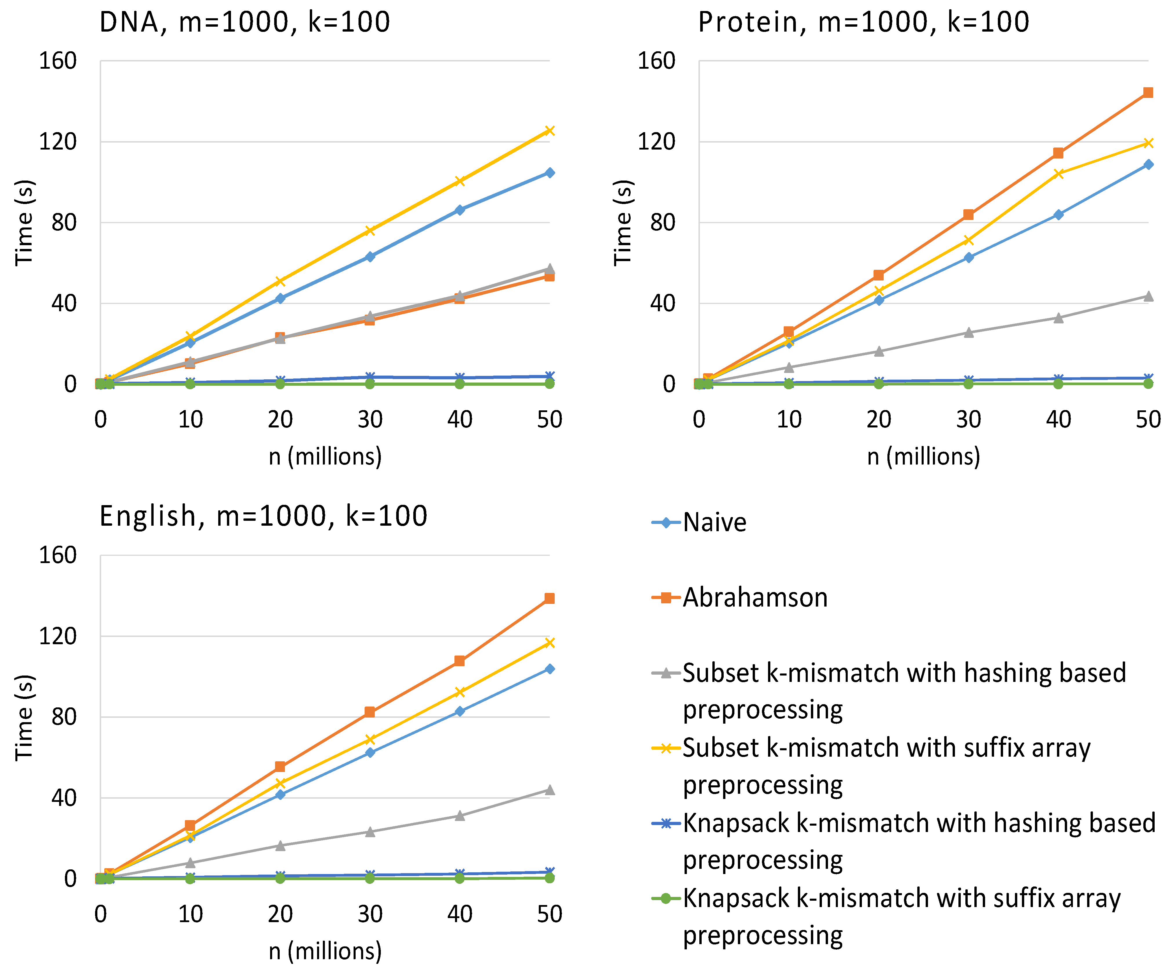
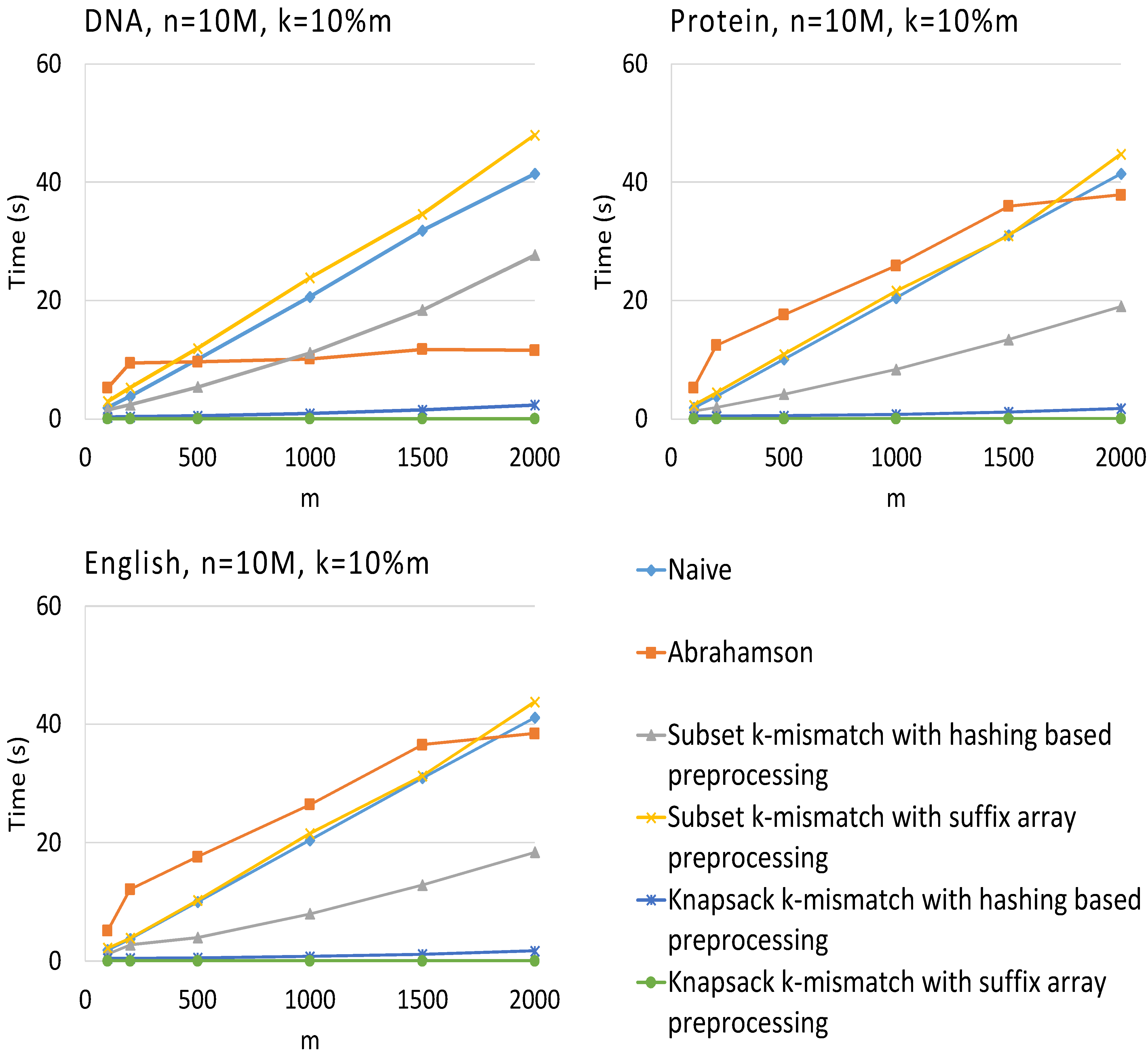
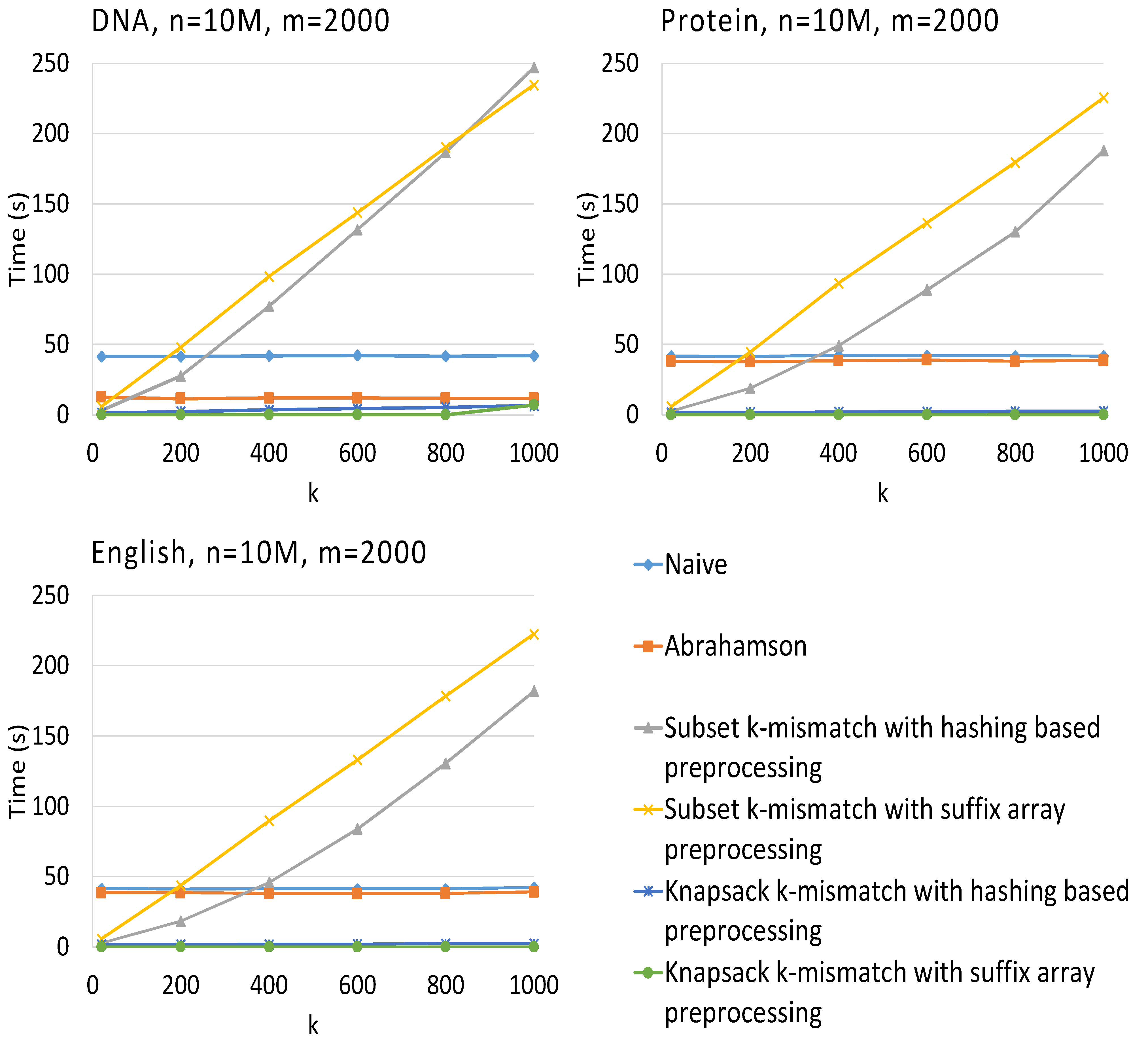
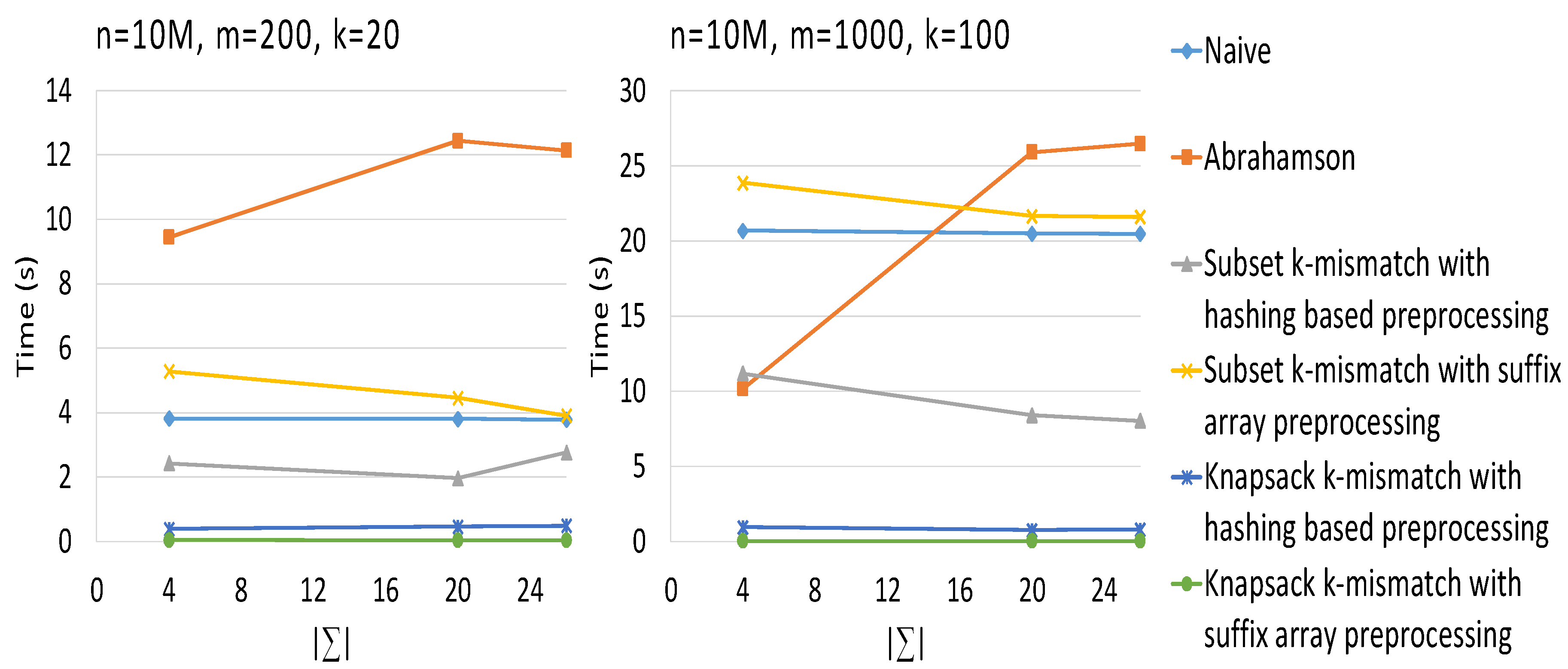
Figure Figure 1 shows run times for varying the length of the text n. All algorithms scale linearly with the length of the text. Figure 2 shows run times for varying the length of the pattern m. Abrahamson's algorithm is expensive, because, for alphabet sizes smaller than , it computes one convolution for every character in the alphabet. The convolutions proved to be expensive in practice, so Abrahamson's algorithm was competitive only for DNA data, where the alphabet is small. Figure 3 shows runtimes for varying the maximum number of mismatches k allowed. The naive algorithm and Abrahamson's algorithm do not depend on k; therefore, their runtime is constant. Subset k mismatch, with its runtime, is competitive for relatively small k. Knapsack k mismatch, on the other hand, scaled very well with k. Figure 4 shows runtimes for varying the alphabet from four (DNA) to 20 (protein) to 26 (English). As expected, Abrahamson's algorithm is the most sensitive to the alphabet size.
Figure 1.
Run times for pattern matching on DNA, protein and English alphabet data, when the length of the text (n) varies. The length of the pattern is . The maximum number of mismatches allowed is . Our algorithms are subset k mismatch with hashing-based preprocessing (Section 2.2.2), subset k mismatch with suffix array preprocessing (Section 2.2.2), knapsack k mismatch with hashing-based preprocessing (Section 2.2.3) and knapsack k mismatch with suffix array preprocessing (Section 2.2.3).

Overall, the naive algorithm performed well in practice, most likely due to its simplicity and cache locality. Abrahamson's algorithm was competitive only for small alphabet size or for large k. Subset k mismatches performed well for relatively small k. In most cases, the suffix array version was slower than the hashing-based one with time pre-processing because of the added factor when searching in the suffix array. It would be interesting to investigate how the algorithms compare with a more efficient implementation of the suffix array. Knapsack k mismatches was the fastest among the algorithms compared, because in most cases, the knapsack could be filled with less than the given “budget”, and thus, the algorithm did not have to perform any convolution operations.
Figure 2.
Run times for pattern matching on DNA, protein and English alphabet data, when the length of the pattern (m) varies. The length of the text is millions. The maximum number of mismatches allowed is of the pattern length. Our algorithms are subset k mismatch with hashing-based preprocessing (Section 2.2.2), subset k mismatch with suffix array preprocessing (Section 2.2.2), knapsack k mismatch with hashing-based preprocessing (Section 2.2.3) and knapsack k mismatch with suffix array preprocessing (Section 2.2.3).

Figure 3.
Run times for pattern matching on DNA, protein and English alphabet data, when the maximum number of mismatches allowed (k) varies. The length of the text is millions. The length of the pattern is . Our algorithms are subset k mismatch with hashing-based preprocessing (Section 2.2.2), subset k mismatch with suffix array preprocessing (Section 2.2.2), knapsack k mismatch with hashing-based preprocessing (Section 2.2.3) and knapsack k mismatch with suffix array preprocessing (Section 2.2.3).

Figure 4.
Run times for pattern matching when the size of the alphabet varies from four (DNA) to 20 (protein) to 26 (English). The length of the text is millions. The length of the pattern is in the first graph and in the second. The maximum number of mismatches allowed is in the first graph and in the second. Our algorithms are subset k mismatch with hashing-based preprocessing (Section 2.2.2), subset k mismatch with suffix array preprocessing (Section 2.2.2), knapsack k mismatch with hashing-based preprocessing (Section 2.2.3) and knapsack k mismatch with suffix array preprocessing (Section 2.2.3).

4. Conclusions
We have introduced several deterministic and randomized, exact and approximate algorithms for pattern matching with mismatches and the k mismatches problems, with or without wild cards. These algorithms improve the run time, simplify or extend previous algorithms wild cards. We have also implemented the deterministic algorithms. An empirical comparison of these algorithms showed that the algorithms based on character comparison outperform those based on convolutions.
Acknowledgments
This work has been supported in part by the following grants: NSF 1447711, NSF 0829916 and NIH R01LM010101.
Author Contributions
Sanguthevar Rajasekaran designed the randomized and approximate algorithms. Marius Nicolae designed and implemented the deterministic algorithms and carried out the empirical experiments. Marius Nicolae and Sanguthevar Rajasekaran drafted and approved the manuscript.
Conflicts of Interest
The authors declare no conflict of interest.
References
- Knuth, D.E.; Morris, J.H., Jr.; Pratt, V.R. Fast Pattern Matching in Strings. SIAM J. Comput. 1977, 6, 323–350. [Google Scholar] [CrossRef]
- Aho, A.V.; Corasick, M.J. Efficient string matching: An aid to bibliographic search. Commun. ACM 1975, 18, 333–340. [Google Scholar] [CrossRef]
- Fischer, M.J.; Paterson, M.S. String-Matching and Other Products; Technical Report MAC-TM-41; Massachusetts Institute of Technology Cambridge Project MAC: Cambridge, MA, USA, 1974. [Google Scholar]
- Indyk, P. Faster Algorithms for String Matching Problems: Matching the Convolution Bound. In Proceedings of the 39th Symposium on Foundations of Computer Science, Palo Alto, CA, USA, 8–11 November 1998; pp. 166–173.
- Kalai, A. Efficient pattern-matching with don't cares. In Proceedings of the thirteenth annual ACM-SIAM symposium on Discrete algorithms; Society for Industrial and Applied Mathematics: Philadelphia, PA, USA, 2002. SODA ’02. pp. 655–656. [Google Scholar]
- Clifford, P.; Clifford, R. Simple deterministic wildcard matching. Inf. Process. Lett. 2007, 101, 53–54. [Google Scholar] [CrossRef]
- Cole, R.; Hariharan, R.; Indyk, P. Tree pattern matching and subset matching in deterministic O(n log3 n)-time. In Proceedings of the Tenth Annual ACM-SIAM Symposium on Discrete Algorithms, Baltimore, MD, USA, 17–19 January 1999; Society for Industrial and Applied Mathematics: Philadelphia, PA, USA, 1999. SODA '99. pp. 245–254. [Google Scholar]
- Navarro, G. A guided tour to approximate string matching. ACM Comput. Surv. 2001, 33, 31–88. [Google Scholar] [CrossRef]
- Navarro, G.; Raffinot, M. Flexible Pattern Matching in Strings–Practical on-Line Search Algorithms for Texts and Biological Sequences; Cambridge University Press: Cambridge, UK, 2002. [Google Scholar]
- Abrahamson, K. Generalized String Matching. SIAM J. Comput. 1987, 16, 1039–1051. [Google Scholar] [CrossRef]
- Amir, A.; Lewenstein, M.; Porat, E. Faster algorithms for string matching with k mismatches. J. Algorithms 2004, 50, 257–275. [Google Scholar] [CrossRef]
- Atallah, M.J.; Chyzak, F.; Dumas, P. A randomized algorithm for approximate string matching. Algorithmica 2001, 29, 468–486. [Google Scholar] [CrossRef]
- Karloff, H. Fast algorithms for approximately counting mismatches. Inf. Process. Lett. 1993, 48, 53–60. [Google Scholar] [CrossRef]
- Clifford, R.; Efremenko, K.; Porat, B.; Porat, E. A black box for online approximate pattern matching. In Combinatorial Pattern Matching; Springer: Berlin Heidelberg, Germany, 2008; pp. 143–151. [Google Scholar]
- Porat, B.; Porat, E. Exact and Approximate Pattern Matching in the Streaming Model. In Proceedings of the (FOCS '09) 50th Annual IEEE Symposium on Foundations of Computer Science; 2009; pp. 315–323. [Google Scholar]
- Porat, E.; Lipsky, O. Improved sketching of Hamming distance with error correcting. In Combinatorial Pattern Matching; Springer: Berlin Heidelberg, Germany, 2007; pp. 173–182. [Google Scholar]
- Clifford, R.; Efremenko, K.; Porat, E.; Rothschild, A. k-mismatch with don't cares. In Algorithms–ESA 2007; Springer: Berlin Heidelberg, Germany, 2007; pp. 151–162. [Google Scholar]
- Clifford, R.; Efremenko, K.; Porat, B.; Porat, E.; Rothschild, A. Mismatch Sampling. Inf. Comput. 2012, 214, 112–118. [Google Scholar] [CrossRef]
- Landau, G.M.; Vishkin, U. Efficient string matching in the presence of errors. In Proceedings of the 26th Annual Symposium on Foundations of Computer Science, Portland, OR, USA, 21–23 October; 1985; pp. 126–136. [Google Scholar]
- Galil, Z.; Giancarlo, R. Improved string matching with k mismatches. SIGACT News 1986, 17, 52–54. [Google Scholar] [CrossRef]
- Clifford, R.; Efremenko, K.; Porat, E.; Rothschild, A. From coding theory to efficient pattern matching. In Proceedings of the Twentieth Annual ACM-SIAM Symposium on Discrete Algorithms, New York, New York, USA, 4–6 January, 2009; Society for Industrial and Applied Mathematics: Philadelphia, PA, USA, 2009. SODA '09. pp. 778–784. [Google Scholar]
- Clifford, R.; Porat, E. A filtering algorithm for k-mismatch with don't cares. Inf. Process. Lett. 2010, 110, 1021–1025. [Google Scholar] [CrossRef]
- Fredriksson, K.; Grabowski, S. Combinatorial Algorithms; Springer-Verlag: Berlin, Germany, 2009; Chapter Fast Convolutions and Their Applications in Approximate String Matching; pp. 254–265. [Google Scholar]
- Chernoff, H. A Measure of Asymptotic Efficiency for Tests of a Hypothesis Based on the Sum of Observations. Ann. Math. Stat. 1952, 2, 241–256. [Google Scholar] [CrossRef]
- Kasai, T.; Lee, G.; Arimura, H.; Arikawa, S.; Park, K. Linear-Time Longest-Common-Prefix Computation in Suffix Arrays And Its Applications; Springer-Verlag: Berlin, Germany, 2001; pp. 181–192. [Google Scholar]
- Bender, M.; Farach-Colton, M. The LCA Problem Revisited. In LATIN 2000: Theoretical Informatics; Gonnet, G., Viola, A., Eds.; Springer: Berlin, Germany, 2000; Volume1776, pp. 88–94. [Google Scholar]
- Ferragina, P.; Manzini, G. Opportunistic data structures with applications. In Proceedings of the IEEE 41st Annual Symposium on Foundations of Computer Science, Redondo Beach, CA, USA, 12–14 November; 2000; pp. 390–398. [Google Scholar]
- Frigo, M.; Johnson, S.G. The Design and Implementation of FFTW3. Proc. IEEE 2005, 93, 216–231. [Google Scholar] [CrossRef]
- Rajasekaran, S.; Nicolae, M. An elegant algorithm for the construction of suffix arrays. J. Discrete Algorithms 2014, 27, 21–28. [Google Scholar] [CrossRef] [PubMed]
© 2015 by the authors; licensee MDPI, Basel, Switzerland. This article is an open access article distributed under the terms and conditions of the Creative Commons Attribution license (http://creativecommons.org/licenses/by/4.0/).
Share and Cite
MDPI and ACS Style
Nicolae, M.; Rajasekaran, S. On String Matching with Mismatches. Algorithms 2015, 8, 248-270. https://0-doi-org.brum.beds.ac.uk/10.3390/a8020248
AMA Style
Nicolae M, Rajasekaran S. On String Matching with Mismatches. Algorithms. 2015; 8(2):248-270. https://0-doi-org.brum.beds.ac.uk/10.3390/a8020248
Chicago/Turabian StyleNicolae, Marius, and Sanguthevar Rajasekaran. 2015. "On String Matching with Mismatches" Algorithms 8, no. 2: 248-270. https://0-doi-org.brum.beds.ac.uk/10.3390/a8020248