Review

Conditional Random Fields for Pattern Recognition Applied to Structured Data

1
Statistical Sciences, Los Alamos National Laboratory, Los Alamos, NM 87544-87545, USA
2
Space Data Systems, Los Alamos National Laboratory, Los Alamos, NM 87544-87545, USA
*
Author to whom correspondence should be addressed.
These authors contributed equally to this work.
Algorithms 2015, 8(3), 466-483; https://0-doi-org.brum.beds.ac.uk/10.3390/a8030466
Submission received: 16 April 2015 / Revised: 17 June 2015 / Accepted: 25 June 2015 / Published: 14 July 2015

Abstract

:
Pattern recognition uses measurements from an input domain, X, to predict their labels from an output domain, Y. Image analysis is one setting where one might want to infer whether a pixel patch contains an object that is “manmade” (such as a building) or “natural” (such as a tree). Suppose the label for a pixel patch is “manmade”; if the label for a nearby pixel patch is then more likely to be “manmade” there is structure in the output domain that can be exploited to improve pattern recognition performance. Modeling P(X) is difficult because features between parts of the model are often correlated. Therefore, conditional random fields (CRFs) model structured data using the conditional distribution P(Y|X = x), without specifying a model for P(X), and are well suited for applications with dependent features. This paper has two parts. First, we overview CRFs and their application to pattern recognition in structured problems. Our primary examples are image analysis applications in which there is dependence among samples (pixel patches) in the output domain. Second, we identify research topics and present numerical examples.

1. Introduction

In pattern recognition problems, there can be dependence among samples in the input domain, or between classification labels of samples in the output domain. For example, fraud detection in credit card transactions relies partly on pattern recognition methods that exploit relations among the samples (transactions), both in the input and output domains [1]. Pattern recognition is commonly applied to unstructured data for which the samples are independent with respect to both the input and output domains, as in Fisher’s well-known iris data [2], consisting of measurements of sepal and petal length and width, from each of many iris plants as input to be used to predict the output (species). In contrast, when there is structure in the input and output domain, i.e., sample input and sample labels are not independent, the problem is referred to as structured machine learning or structured prediction. Several similar terms, including classification, pattern recognition, prediction, and machine learning are used in various technical fields (statistical science, computer science, information science, and various engineering fields) to describe the task of using predictor features (also known as predictors or independent variables) to predict a response. Some examples of structured machine learning include fraud detection in credit card transactions and object recognition in images i.e., labeling pixels or pixel patches (also known as superpixels) in images.
A broad category of models, known as probabilistic graphical models (PGMs) is being increasingly used to model problems having a structured domain [3]. PGMs are represented by two main categories of models. Directed graphical models are known as Bayesian Networks (BNs) and undirected graphical models are known as Markov random fields (MRFs) and conditional random fields (CRFs). PGMs are used to express dependencies between the input and output domains, as well as dependencies within domains, and to enable probabilistic inferences such as answering queries about the output variables using the probabilistic model (e.g., a model based on a CRF, a MRF or a BN) of the problem. A key task is to compute the probability distribution over the variables of interest (for a test sample called the query), given the observed values of other random variables (the evidence).
CRFs were introduced by Lafferty et al. [4] for modeling structured data. Since then CRFs have been successfully applied in a broad range of applied domains such as bioinformatics [5,6,7], computer vision [6,7,8,9,10,11,12,13,14,15,16], assessment of climate change impact [17], active learning [18,19], and natural language processing [4,20,21,22]. A good introduction on CRFs is given in [23]. In addition to describing research directions, this paper reviews recent work, outlines the main challenges in learning CRFs, and provides examples of approximate inference, with a focus on a decomposition approach that uses spanning tree based approximations of the original graph model.
While a Markov Random field (MRF) models the joint probability distribution, P(Y,X), and includes a model for P(X), a CRF directly models a conditional distribution, P(Y|X = x), without specifying a model for P(X). In general, modeling P(X) is difficult because feature functions between parts of the model are often correlated. As a result of direct modeling of conditional distributions, CRFs have been found well-suited to process rich, dependent features without having to model P(X). Figure 1 illustrates results of object recognition using MRFs and CRFs for man-made object detection [8]. Figure 2 illustrates the Y and X values for an image similar to the image in Figure 1. We used the dataset that was presented in Kumar and Hebert [8,9]. The dataset contains 108 training and 129 testing images, each of size 256 × 384 pixels, from the Corel image database. Each image was divided into non-overlapping patches of 16 × 16 pixels. The goal was to label each patch as structured (man-made) or non-structured (natural background). The X and Y values corresponding to these images, are available from [8], but the meaning of X and Y are reversed in [8] from that used here. We use X to denote the input predictors, which in this example includes intensity gradients in different spatial orientations. Figure 2 illustrates the reference labeling and feature vectors corresponding to 16 × 16 pixel patches.
Figure 1. Example of man-made objects in a natural scene. Pixel patches (16 × 16 pixels) containing man-made structures are outlined. (a) MRF result; (b) CRF result.
Algorithms 08 00466 g001
Figure 2. Illustration of reference labeling and corresponding feature values. The image is 16 × 24 elements, where each element represents a 16 × 16 pixel patch in the original image of 256 × 384 pixels from [8]. (a) The Y labels (0 = red for natural, 1 = white for manmade); (b) The corresponding X values represented using a scalar (projection of X onto the first eigenvector of the covariance matrix of X; i.e., the first principle component scores; see Section 3). (a) Y values by pixel: Red is “natural” (0) White is “manmade” (1); (b) Scalar representation of X values at the same pixels as in plot (a).
Algorithms 08 00466 g002
This paper has two main parts. First, we provide an overview of CRFs and their application to pattern recognition. Our primary examples are image analysis applications in which there is dependence among samples (pixels or pixel patches) in the output domain since nearby samples tend to have similar labels such as “natural” or “manmade”. Second, we point out successful applications of CRFs, identify open research topics, and present numerical performance examples. The paper is organized as follows: Section 2 describes CRFs, including their assumptions, and options for learning (estimating) model parameters; Section 3 describes applications of CRFs, and challenges in CRF applications; Section 4 gives examples to illustrate pattern recognition performance using CRFs; and Section 5 describes open research topics related to CRFs. Section 6 is a summary.

2. Conditional Random Fields

In the CRF model, the conditional probability distribution is factored according to a graph consisting of a set of nodes, Y, and a set of edges, E. The nodes represent random variables, y i , that take values in a finite set of classification labels. Inter-node edges encode dependency relations among the random variables. The corresponding observation variable, x i , could be, for example, average intensity or color vector (red, green, blue) of the pixel patch at the position i, and the variable y i = { 0 , 1 } could represent whether the pixel patch contains man-made structures. It should be noted that the CRF-based approach relaxes the assumption of conditional independence of the observed data; thus, the observation variables x i and x j can include components, which are dependent. For example, the observation variable x i could include average intensities and/or intensity gradients over the pixel patch, i, and over neighboring pixel patches. In contrast to the MRF model, the CRF model relaxes the restrictive assumption of conditional independence of the observations in MRFs. This allows a convenient factorization that makes efficient modeling possible.
By the Hammersley and Clifford theorem [24], under the mild assumption that P(Y|X;θ) > 0 for all possible Y values, in a CRF, the conditional probability distribution can be given in a factored form as:
P ( y | x ) = 1 z(x) c C ψ c ( y c , x c , θ )
where z ( x ) = y Y c C ψ c ( y c , x c , θ c ) xc is a feature vector, ψ c are factors that are specified for the application (see below), and yc are the corresponding labels.
In Equation (1), the factors ψc correspond to maximal cliques in the graph and is usually a member of the exponential family. The term C is the set of all maximal cliques in the graph, where a maximal clique of a graph is a fully connected subset of nodes that cannot be further extended. The function z(x) is the partition function required for P(y|x) to sum to one over all possible values of y. We use lower case letters to depict realized values of the corresponding random variables (which are upper case). We give particular examples of Equation (1) in Equations (2) and (3) below.
The probability P(Y|X;θ) must sum to 1 over all possible values of the Y vector The partition function, Z, is difficult to calculate because enforcing the normalization y P ( Y | X ; θ ) = 1 requires a summation over 2 n 2 pixels in the case of an n-by-n square image for a binary-valued class label Y, which is computationally nearly impossible for modest values of n such as n = 100. The vector Y = { y 1 , y 2 , ... , y n 2 } is the vector of class labels (one label for each pixel).
In applications, e.g., computer vision, a pairwise CRF model is often used. This model takes into consideration only unary and pairwise cliques. The distribution is then defined as
P ( Y | X ; θ ) = 1 Z ( X ; θ ) i V ψ i ( Y i , X ;   θ i ) ( i , j ) E ψ i j ( Y i , Y j , X ;   θ i j )
and can be rewritten as
P ( Y | X ; θ ) = 1 Z exp ( i S ψ i ( y i , X , θ ) + i S j N i ψ i j ( y i , y j , X , θ ) )
where θ is the parameter vector, Z is the partition function that is used to ensure that y P ( Y | X ; θ ) = 1 , S indexes CRF nodes that correspond to random variables, ψi is the association (also called pairwise) potential (usually a function in the exponential family) involving individual samples, and ψij is the interaction potential (usually a function in the exponential family) involving samples in the neighborhood Ni of site “i.” If we consider only the association potential term ψi, the model reduces to the logistic regression. The introduction of the interaction ψij potential accounts for the fact that interlinked random variables impact each other’s states. Example applications of CRFs that use pairwise cliques in computer vision include [8,9] and many others.
Now that Equation (2) is introduced, we point out that the term “inference” can either include all aspects of model formulation, including choosing a model, choosing a neighborhood structure, estimating the corresponding model parameters, and the final step of inferring the class label of a sample (see Section 4 and Section 5). In Equation (2), this means one must choose the association and interaction potential functions, the neighborhood structure, and then some type of estimation method to estimate the model parameters θ. We point out, however, that in the PGM literature, “inference” is not such a broad term, but refers only to computing the probability distribution over the unobserved variables y i Y given the observables, which include values for Xs and possibly some subset of Y. A sample label is then inferred based on the computed probability distribution. In the statistics literature, “inference” is the broader task of choosing a model and estimating the model parameters. This paper clarifies with each usage the meaning of the term “inference”. Schemes for parameter estimation in CRFs are described in Section 2.1.
It is known that inference in general graphical models is NP-hard, unless the models have tree-like structures or the model size is small [25,26]. Probabilistic inference in CRFs based on trees is computationally efficient and exact. However, the expressiveness of a tree-structured model for approximating a general probabilistic graphical model is limited. A challenge in CRF model structure construction and parameter optimization (learning) is to balance the expressive power of the models with the computational complexity of inference in the models, because the inference has to be performed both during model learning and for answering probabilistic queries based on the optimized model. This requires developing computationally-efficient inference algorithms that provide a reasonable approximation to the inference over the original computationally-intractable model. A growing effort in recent years has been devoted to developing approximate probabilistic inference algorithms that can broadly categorized as: (1) variational algorithms, that cast the inference problem as an optimization problem. This category includes the mean-field approach [27], energy minimization using loopy belief propagation (LBP) [28,29,30,31], generalized belief propagation [32,33], tree reweighted approaches for maximum posterior marginals (MPM) estimation and maximum a posteriori (MAP) inference [34,35,36], and linear programming relaxations of MAP estimation [37,38,39,40,41] and (2) techniques that constrain the original problem using methods such as graph cuts [25,42,43]. The graph cuts technique introduces submodularity constraints and casts the inference over a general graph as finding the MAP configuration over the constrained graphical model. Submodular problems belong to a more general class of linear programming relaxation techniques. Ongoing research in this area focuses on estimating uncertainties associated with the graph cuts output [44] and scaling the technique to larger problems, including multi-class classifications [45,46,47,48].

2.1. CRF Learning

In general, learning the CRF model includes choosing a graphical model structure and estimating parameters corresponding to the chosen structure. Assuming that the structure is given, e.g., defined using domain expertise, learning the CRF model corresponds to finding the model parameters θ * that maximize the conditional log-likelihood objective, L, on the training data D,
θ * = arg max θ L ( D , θ ) = arg max θ ( 1 | D | ( X , Y ) D log P ( Y | X ; θ ) λ | | θ | | 2 )
where the regularization penalty term λ | | θ | | 2 ( λ = 1 / 2 σ 2 ) is a Gaussian, prior imposed on the parameters to control for overfitting, and | D | is the size of the training data set. Estimation of the gradient of the log-likelihood objective requires computing marginals and is usually not tractable due to the presence of the partition function Z. Approximate computation of the marginal probabilities can be performed using LBP. The model parameters are often initialized using maximum likelihood estimation for the logistic regression model. Then, a limited memory quasi-Newton method, such as L-BFGS [49], is used to estimate the parameters. Once the model parameters are estimated, inferring classification labels is done using either maximum a posteriori (MAP) or the maximum posterior marginals (MPM) criteria that, similar to learning, require computing marginals and the partition function. To reduce the computational complexity of model learning, alternative objectives for learning have been proposed, including pseudo-likelihood (see Section 2.1.2) and contrastive divergence [10,50,51,52,53].

2.1.1. Estimation of Model Parameters θ Using Markov Chain Monte Carlo

The broad topic of inference schemes based on Markov Chain Monte Carlo [54] (MCMC) for CRFs are another type of approximate inference, because numerical methods are used to approximate the true posterior distribution of each CRF model parameter. Here, the term “approximate inference” refers to approximate methods to estimate CRF model parameters; there are several interpretations of approximate inference, depending on whether the likelihood is somehow approximated, or the estimation scheme is an approximate one based on the approximate or true likelihood.
In many models, one relatively straightforward option to estimate model parameters θ is a numerical Bayesian option such as MCMC. In fact, if Z were a known function of the unknown θ in Equation (2), then standard implementation MCMC which requires knowledge only of the ratio of probabilities (see the next paragraph) would be a good option to avoid having to compute Z [50,51]. MCMC examines many candidate parameter values θ′ and accepts those candidate values as an observation from the posterior distribution with a probability that depends on the value P ( Y | X ; θ ) P ( Y | X ; θ c u r r e n t ) × Z ( θ ) Z ( θ ) . Because MCMC accepts a finite number of candidate θ′ values, the MCMC-based posterior has approximation error, even in situations where Z is a known function of the unknown θ in Equation (2). Also, in any application of MCMC, one must check whether the chain has converged to the posterior distribution [50,54].
For situations such as CRFs where the ratio P ( Y | X ; θ ) P ( Y | X ; θ current ) depends on the unknown ratio, Z(θ)/Z(θ′), one of the first approximate estimation options developed was reverse logistic regression [55]. In parameter estimation for CRFs, suppose we have a collection of m normalizing constants, Z(θ1),Z(θ2),…,Z(θm), simply by trying different values of θ on a grid of values. For each value of θ denoted θk, MCMC can be used to generate random samples each of size n from the unnormalized (does not sum to 1) distribution denoted here as P(Y|Xk), and P(Y|Xk) = P′(Y|Xk)/Zk. The collection P′(Y|X1), P′(Y|X2),…, P′(Y|Xm) can be combined as in mixture distributions as j = 1 m P ( Y | X ; θ 1 ) e η j , where e η j is introduced to satisfy η j = log ( Z k ) + log ( n n m ) = log ( Z k ) + log ( 1 m ) and then p k ( Y | X ; θ k ) = P ( Y | X ; θ k ) e η k k = 1 m P ( Y | X ; θ k ) e η k is the probability that a simulated value Y from the mixture probability j = 1 m P ( Y | X ;   θ 1 ) e η j occurred in the jth sample (there are mn samples) in the mixture distribution. Reverse logistic regression can then be applied to the n samples from each of P′(Y|X1), P′(Y|X2),…, P′(Y|Xm) to estimate the ηj values, which determine the normalizing constants Zk. For the mn samples Yij, the likelihood for reverse logistic regression is l ( η 1 , η 2 , ... , η m ) = j = 1 m i = 1 n j log ( p j ( Y i j , η 1 , η 2 , ... , η m ) ) , which can be maximized to solve to the estimate the ηj values. This use of reverse logistic regression involves approximating the normalizing constants, Zk, so it is one type of approximate inference.

2.1.2. Estimation of Model Parameters θ Using Pseudo-Likelihood or Composite-Likelihood Methods

Besag [24,56] introduced pseudo-likelihood and Lindsey [57] introduced composite-likelihood methods. These methods do not attempt to maximize the full likelihood, but instead maximize some type of conditional likelihood. For Gaussian MRFs, [58] compared pseudo-likelihood to the full likelihood for small numbers of pixels under varying amounts of simulated non-Gaussian behavior. For CRFs, [59] maximized the pseudo-likelihood.
P L ( Y | X ; θ ) = i = 1 n 2 log ( P ( y i | y N i , x ; θ ) )
where Equation (2) is written as P ( Y | X ; θ ) = 1 Z a = 1 A ψ a ( y a , x a ; θ ) for appropriate choice of A and ψ a .
Equation (3) is not the full likelihood for a CRF, but is a likelihood conditioned on the neighboring true Y values in training data. Similarly, [60] applied composite likelihood to Gibbs fields, and a very similar approach could work for CRFs, due to the equivalence of Gibbs fields and MRFs and the fact that CRFS are MRFs when conditioned on the global observation vector, X.

2.1.3. Estimation of Model Parameters θ Using Likelihood-Free Methods

In the context of the Potts random field, [61] provided a likelihood-free option to deal with the fact that the ratio P ( Y | X ; θ ) P ( Y | X ; θ current ) depends on the unknown ratio Z ( θ ) Z ( θ ) . The likelihood-free option is related to the auxiliary variable method, both of which generate samples from approximate densities. The likelihood-free methods introduce an auxiliary random vector so that synthetic samples can be simulated (without having an explicit analytical form for the likelihood) that have the correct asymptotic distribution, and thus circumvent the issue of having intractable likelihoods inside a MCMC loop. The Potts random field extends the well-known Ising model (see Section 3 for an application in image denoising) that originated to describe magnetic properties in statistical physics by allowing multiple possible instead of binary possible values for Y.

3. CRF Applications and Challenges

In a typical CRF graphical model, the class labels at the graph node given the observed data are assumed to obey a predefined dependence structure. A Markov dependence structure (see below) is one for which the class label at node i depends on the class labels in the neighborhood of node i. Additionally, the class label at the node i depends on “compatibility” of feature vectors corresponding to the node i and its neighbors in the neighborhood. Natural language processing extracts syntax from text, often to aid search and to find related documents. The response variable, Y, is a part-of-speech tag and the predictors, X, include information about the word at a given position, such as its identity and memberships in domain-specific lexicons. One common goal in computer vision is to classify regions in an image, and as Figure 1 suggests, the Y labels near a given pixel, i, influence our beliefs about Yi, as is captured in the neighborhood structure in Equation (1).
A particular example of Equation (1) for 2-dimensional image data is
P ( Y = 1 | X ; θ ) = 1 Z exp ( i S w T ψ i ( y i ) x i + i S j N i v T ψ i j ( y ) x i x j )
In Equation (4), ψ i ( y i ) = ( 1 , y i ) , a two-component vector and ψ i j ( y ) = ( 1 , | y i y j | ) , also a 2-component vector, and the xi are all two-dimensional. The model parameter vector θ = ( w , v ) .The application for Equation (4) in [50,51] was image segmentation, which partitions or clusters an image into homogeneous pixels or pixel patches such as “land” or “water”.
One well-known MRF that has many applications, including image denoising, is the Ising model [58,61,62]. In the image denoising context, the interaction portion of Equation (2), i S j N i ψ i j ( y i , y j , X , θ ) can be regarded as being a prior probability for the true Y values. Such a prior probability can enforce a tendency for neighboring Y values to be similar or dissimilar, depending on the application. The term i S φ i ( y i , X , θ ) in Equation (2) can be regarded as the likelihood, choosing, for example, ψ i = exp { θ ( y i x i ) } 2 , where yi = xi + ei with xi the true image value, ei, the measurement errors, and neighboring yi, predicted to be similar or dissimilar by choice of ψ i j ( y i , y j , X , θ ) .
Despite the computational issues described in Section 2, CRFs have proven to perform well for many applications. For example, [8] demonstrates good CRF performance compared to other pattern recognition methods such as a Gaussian mixture model or support vector machines [63] in labeling pixel patches as natural or manmade. Furthermore, a few papers, such as [50,51], show how well the various approximation schemes work in limited settings with experimental data.
Aside from the need for better and faster approximate inference methods for CRFs, another open issue is choosing a model structure by using prior knowledge about the domain or by using trial and error with different structures. In the context of hidden Gibbs random fields, [64] recently developed a method to choose the dependency structure in Gibbs fields that relies on approximate Bayesian computation. Another way to assess candidate model structure (such as function forms or number of connections used in Equation (1)) is empirical classification accuracy. Choosing the model structure involves choosing the number of layers in the model, the structure of each layer, as well as the number of states of the latent variables in the hidden layers. Naturally, the probabilistic inference is an unavoidable component in estimating changes the model structure. The idea of capturing the multiscale nature of the problem of interest, such as image modeling, is naturally related to the structure learning. For instance, image modeling using a multi-layer CRF was proposed by [10]. Reference [65] extended the CRF framework by incorporating structured hidden variables to model components (parts) constituting objects; this extension became known as hidden CRFs (HCRFs). A non-parametric model that is capable to automatically learn the number of hidden states in HCRFs was presented in [15]. Reference [13] introduced class of energies with hierarchical costs to model classification labels organized in a hierarchy.

4. Examples

This section describes performance in two example applications of CRFs in computer vision domain. These examples include performance evaluation of the original 2D grid structured CRF model with LBP inference, and CRF model approximations based on spanning trees, pseudo-likelihood and graph cuts. For comparison we show performances demonstrated by MRF, logistic regression models and mixture discriminant analysis.

4.1. Example 1: Pattern Recognition to Distinguish Natural from Manmade Objects

Using data available from [8], from which the images in Figure 1 and Figure 2 were created, with 108 training and 129 testing images such as those shown in Figure 1 and Figure 2, [66,67] give misclassification rates for several methods, including existing CRF-based methods and CRF model approximations using an ensemble of spanning trees (Figure 3) or a cascade of spanning trees. The X vector consists of image gradients and is 14-dimensional at each pixel. The false positive (predicting a pixel that really is a natural object to be man-made) and false negative rates (predicting a pixel that really is man-made to be natural) are given separately. The results are summarized in Table 1 and illustrated in Figure 4. Because the false positive rates were not the same for all methods in testing, we do not attempt to declare a winning method, but only to illustrate strong performance by several methods. It should be noted, though, that the cascade model built of tree-structured approximations performed better than the grid-structured CRF with LBP inference both in terms of detection rate and false positive rate.
Figure 3. Illustration of a 5 × 7 grid-like CRF graph (a) and corresponding two randomly generated spanning trees (b,c). In CRF setup in computer vision, the observation variable X i j could be the average color of the pixel patch, and the random variable Y i j is a classification label of the pixel patch. For clarity we show only one pair of X i j and Y ij .
Algorithms 08 00466 g003
Figure 4. Example results for structure detection task. True positives are brightened and outlined with white boundaries.
Algorithms 08 00466 g004
Table 1. Detection rates (DR) and false positives per image (FP) for structure detection problem over the test set containing 129 images. Comparisons to Markov random field, and grid-structured CRF model with loopy belief propagation inference (LBP) are also shown.
DR (%)FP (Per Image)
Markov Random Field [9]58.352.44
Discriminative Random Fields [9]72.541.76
LBP (MPM estimates)85.3014.32
Ensemble of spanning tree structured CRFs [66]90.529
Hierarchical cascade of spanning tree structured CRFs (MPM estimates) [67]91.7511.85

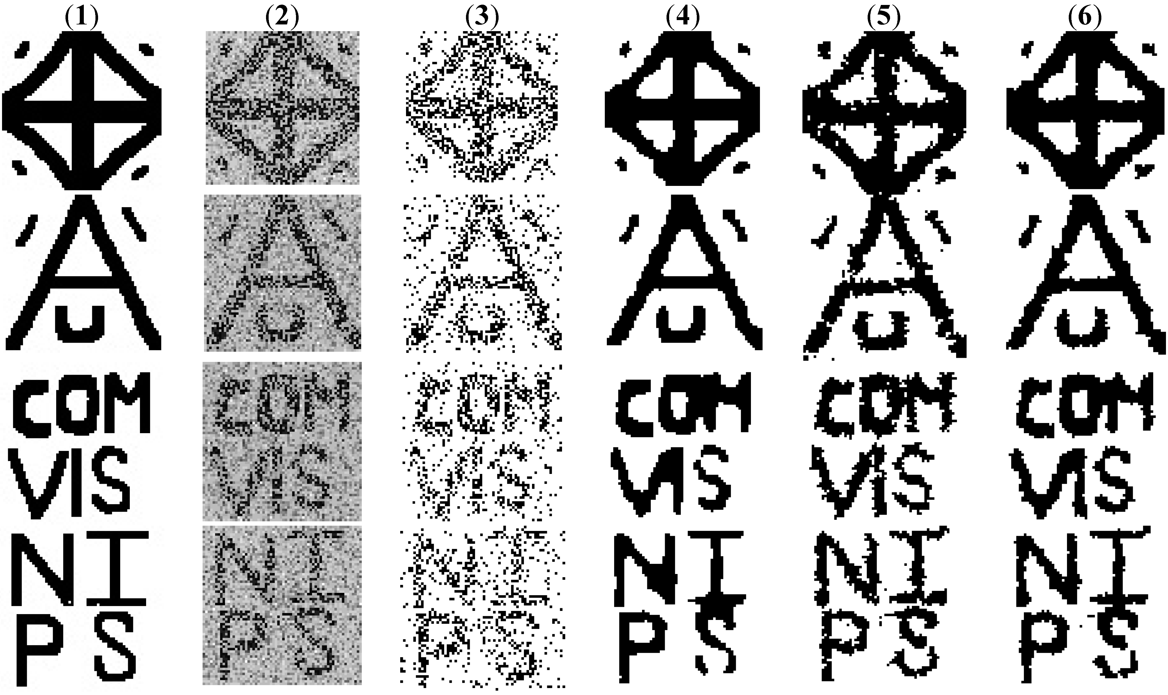
4.2. Example 2. Image Denoising

References [66,67] also analyzed noisy images, such as that shown in Figure 5. The synthetic noise was either unimodal Gaussian or bimodal Gaussian. The data are from [8], and [66,67] find good performance (low pixelwise misclassification rate) for LBP, the new CRF method using the ensemble of spanning trees of 6.21%, 6.04%, and 5.80%, respectively (for the bimodal Gaussian noise). A logistic regression classifier performed noticeably worse, with 23.1% pixelwise classification error. These results are summarized in Table 2. It is evident that the approximation based on the ensemble of spanning tree structured CRFs demonstrates better performance than the ones produced by the grid-structured CRF model that uses LBP inference, and the models in [9] in the case of bimodal noise.
Figure 5. Results of binary denoising task. Column (1) reference images; (2) images corrupted with bimodal noise; (3) logistic classifier results; (4) results of the grid structured CRF model with loopy belief propagation inference; (5) result using one spanning tree; (6) CRF spanning trees cascade results.
Algorithms 08 00466 g005
In the second part of this Example 2, we introduce new results from a relatively simple alternative to CRFs in order to denoise the images that contain the bimodal Gaussian noise that has two key aspects. The first aspect exploits the knowledge that the errors are bimodal; that is, because the added synthetic noise was bimodal in one case, we fit a mixture distribution, using the function mda, which implements mixture discriminant analysis (MDA) in R [68]. The second aspect is that we exploit structure simply by smoothing the estimates y ^ from MDA of each pixel, which approximates the behavior of CRFs. If the smoothed prediction exceeds 0.5, we predict a 1; if the smoothed prediction is less than or equal to 0.5, we predict a 0. We also tested neighborhood sizes, trying 3 × 3, 5 × 5, or 7 × 7 neighborhood sizes. A size-3 neighborhood is the 3-by-3 square block of pixels centered on the target pixel, and similarly for the size-5 and size-7 neighborhoods. Pixels near the edge of the scene have truncated neighborhoods.
Table 2. Pixelwise classification error (%) for binary denoising task. KH’06 stands for the results published in [9]. Comparisons to logistic classifier and grid-structured CRF model with loopy belief propagation inference (LBP) are also shown. The averaging was done over five different runs each on 160 test samples; mean ± standard deviation is shown.
UnimodalBimodal
Logistic regression based classifier14.72 ± 0.0223.10 ± 0.04
KH’06 (DRF, penalized pseudo-likelihood parameter learning, MAP labelings estimated using graph cuts)2.306.21
LBP (MPM estimates)2.65 ± 0.116.04 ± 0.09
Ensemble of spanning tree structured CRFs [66]3.38 ± 0.045.80 ± 0.02
Hierarchical cascade of spanning tree structured CRFs [67]3.06 ± 0.116.00 ± 0.12
First, using MDA, on a per-pixel basis without exploiting any structure in Y, the testing error rate is 14%. Next, we exploited the structure in Y by smoothing. If we simply used the average values of the neighboring pixels, the testing error averaged approximately 5%, 5%, and 5% (repeatable to within less than ±1% as in Table 2) results for 3-nbr, 5-nbr, or 7-nbr, respectively. If we first applied MDA to get an initial estimate of each Y, and smoothed those estimates, the testing error averaged approximately 4%, 3%, and 4% for 3-nbr, 5-nbr, or 7-nbr, respectively. Therefore, this is a case where it helps to know the error structure, because this simple approach is competitive with the CRF approaches. However, one could argue that it is unfair to use MDA in this context, because MDA allows for the known bimodal error structure. Nevertheless, this suggests that it can be important to estimate the error structure from training data, which is a topic for future work, and would involve goodness-of-fit testing to select CRF models that are most supported by the data. Additionally, there might be computer-run-time reasons to prefer the simpler-than-CRF approach However, these results were obtained in R on a modern desktop PC, so the computer run times for this simple approach that uses smoothing and MDA cannot yet be meaningfully compared to run times for CRFs that were implemented on another desktop.

5. Research Issues for CRFs

First, regarding the computational challenges discussed in Section 2, there are open problems for maximum posterior marginal (MPM) estimation and maximum a posteriori (MAP) estimation. The lack of MPM and MAP inference methods that scale up to large data sets severely limits CRF usage. Most of the current approaches to address this challenge focus on approximate inference schemes, e.g., using either approximate optimization function, approximations of the original graph model such as spanning trees or the region graphs, or introducing constraints such as submodularity employed in the graph cuts approach.
Second, the MDA performance in Example 2 in Section 4 suggests that it would be valuable to accommodate different forms for the CRF likelihood in models such as Equations (1)–(3). In Example 2, we know that the true distribution of the feature vector, X, is bimodal (a mixture of two Gaussians, which is not in the exponential family), so one could select the association potential terms ψ i , and/or the interaction terms ψ i j in Equation (2) to better accommodate mixture distributions, which are quite general, and can approximate many real-life error distributions.
Third, and related to the second, is goodness of fit testing. Cross-validation allows us to evaluate the classification performance of the model. However, it does not show how accurately the learned model captures the target distribution. We are not aware of any efforts to use a fitted CRF to generate simulated data (generate Y’s conditional on X), re-apply each candidate estimation strategy, and then see how well the inferred model parameters agree with the true and known model parameters. Given an ability to simulate from a fitted CRF (probably using some type of MCMC strategy as in [69]), goodness of fit tests could be developed, perhaps extending the goodness of fit tests proposed in [70]. Because CRFs have many choices such as the neighborhood structure, and the particular parametric functions φ i and ψ i j in Equation (2), it is important to have a way to assess the quality of the fitted CRF to model the real data. Of course, any CRF can be used for pattern recognition, but if such a simulation-based goodness of fit test indicated a lack of fit, then it is reasonable to assume that a CRF with different modeling assumptions would have a better classification performance in pattern recognition.
In summary, three important issues are: (1) developing efficient approximate probabilistic inference in general graphs (e.g., MCMC with reverse logistic regression, generalized belief propagation, decomposition approaches such as tree based approximations of the original general graphical model, and linear programming relaxations of the MAP estimation problem); (2) learning CRF structure simultaneously with estimating CRF parameters; and (3) goodness-of-fit testing. The first issue is a challenge of utmost importance in graphical probabilistic models. The second and third issues depend on the solution of the first issue because it is currently difficult to evaluate many candidate structures and introduce optimal changes to a given structure.

6. Conclusions

Conditional random fields (CRFs) model structured data using the conditional distribution P(Y|X = x), without specifying a model for P(X), and are well suited for applications with dependent features. This paper had two parts. Part one overviewed CRFs and their application to pattern recognition in structured problems. Our primary examples were image analysis applications in which there is dependence among samples (pixel patches) in the output domain because nearby pixel patches tend to have similar labels such as “natural” or “manmade”. Part two described successful applications of CRFs, presented numerical examples, and identified research topics. Regarding research topics, computational challenges in fitting CRFs are being addressed using approximate learning methods. Some of those approximation methods were described, and others are under development. Fortunately, even a suboptimal fit of CRF parameters has the potential to perform specific tasks fairly well. Nevertheless, we anticipate that goodness of fit testing, which currently is non-existent in the CRF literature, will improve CRF model selection and improvement.

Acknowledgments

We acknowledge Los Alamos National Laboratory’s directed research and development (LDRD) for funding this work.

Author Contributions

Both authors contributed equally to this work.

Conflicts of Interest

The authors declare no conflict of interest.

References

  1. Bolton, R.; Hand, D. Statistical fraud detection: A review. Stat. Sci. 2002, 17, 235–255. [Google Scholar]
  2. Fisher, R. The use of multiple measurements in taxonomic problems. Ann. Eugen. 1936, 7, 179–188. [Google Scholar] [CrossRef]
  3. Koller, D.; Friedman, N. Probabilistic Graphical Models: Principles and Techniques; MIT Press: Cambridge, MA, USA, 2009. [Google Scholar]
  4. Lafferty, J.; McCallum, A.; Pereira, F. Conditional random fields: Probabilistic models for segmenting and labeling sequence data. In Proceedings of the 18th International Conference on Machine Learning, Williamstown, MA, USA, 28 June–1 July 2001.
  5. Sato, K.; Sakakibara, Y. RNA secondary structural alignment with conditional random fields. Bioinformatics 2005, 21, ii237–ii242. [Google Scholar] [CrossRef] [PubMed]
  6. Hayashida, M.; Kamada, M.; Song, J.; Akutsu, T. Prediction of protein-RNA residue-base contacts using two-dimensional conditional random field with the lasso. BMC Syst. Biol. 2013. [Google Scholar] [CrossRef] [PubMed]
  7. Sankararaman, S.; Mallick, S.; Dannemann, M.; Prufer, K.; Kelso, J.; Paabo, S.; Patterson, N.; Reich, D. The genomic landscape of Neanderthal ancestry in present-day humans. Nature 2014, 507, 354–357. [Google Scholar] [CrossRef] [PubMed]
  8. Kumar, S.; Hebert, M. Discriminative fields for modeling spatial dependencies in natural images. In Advances in Neural Information Processing Systems 16; Proceedings of the Neural Information Processing Systems, Vancouver, British Columbia, Canada, 8–13 December 2003.
  9. Kumar, S.; Hebert, M. Discriminative random fields. Int. J. Comp. Vis. 2006, 68, 179–201. [Google Scholar] [CrossRef]
  10. He, X.; Zemel, R.; Carreira-Perpinan, M. Multiscale conditional random fields for image labeling. In Proceedings of the IEEE Conference on Computer Vision and Pattern Recognition, Washington, DC, USA, 27 June–2 July 2004; Volume 2.
  11. Reiter, S.; Schuller, B.; Rigoll, G. Hidden conditional random fields for meeting segmentation. In Proceedings of the International Conference on Multimedia and Exposition, Beijing, China, 2–5 July 2007; pp. 639–642.
  12. Ladicky, L.; Sturgess, P.; Alahari, K.; Russell, C.; Torr, P. What, where and how many? Combining object detectors and CRFs. In Proceedings of the European Conference on Computer Vision, Hersonissos, Greece, 5–11 September 2010.
  13. Delong, A.; Gorelick, L.; Veksler, O.; Boykov, Y. Minimizing energies with hierarchical costs. Int. J. Comp. Vis. 2012, 100, 38–58. [Google Scholar] [CrossRef]
  14. Pellegrini, S.; Gool, L. Tracking with a mixed continuous-discrete conditional random field. Comp. Vis. Image Underst. 2013, 117, 1215–1228. [Google Scholar] [CrossRef]
  15. Bousmalis, K.; Zafeiriou, S.; Morency, L.; Pantic, M. Infinite hidden conditional random fields for human behavior analysis. IEEE Trans. Neural Netw. Learn. Syst. 2013, 24, 170–177. [Google Scholar] [CrossRef] [PubMed]
  16. He, X.; Gould, S. An exemplar based CRF for multi-instance object segmentation. In Proceedings of the IEEE Conference on Computer Vision and Pattern Recognition, Columbus, OH, USA, 24–27 June 2014.
  17. Raje, D.; Mujumdar, P. A conditional random field based downscaling method for assessment of climate change impact on multisite daily precipitation in the Mahanadi basin. Water Resour. Res. 2009, 45, 20. [Google Scholar] [CrossRef]
  18. Martinez, O.; Tsechpenakis, G. Integration of active learning in a collaborative CRF. In Proceedings of the IEEE Computer Vision and Pattern Recognition Workshops, Anchorage, AK, USA, 23–28 June 2008.
  19. Zhang, K.; Xie, Y.; Yang, Y.; Sun, A.; Liu, H.; Choudhary, A. Incorporating conditional random fields and active learning to improve sentiment identification. Neural Netw. 2014, 58, 60–67. [Google Scholar] [CrossRef] [PubMed]
  20. Sha, F.; Pereira, S. Shallow parsing with conditional random fields. In Proceedings of the Conference of the North American Chapter of the Association for Computational Linguistics on Human Language Technology, Edmonton, Canada, 31 May–June 1 2003; pp. 134–141.
  21. Sutton, C.; McCallum, A. Piecewise training for undirected models. In Proceedings of the Conference on Uncertainty in Artificial Intelligence, Edinburgh, UK, 26–29 July 2005.
  22. Ammar, W.; Dyer, C.; Smith, N.A. Conditional random field autoencoders for unsupervised structured prediction. In Advances in Neural Information Processing Systems 27 (NIPS 2014), Proceedings of the Neural Information Processing Systems, Montreal, Canada, 8–13 December 2014.
  23. Sutton, C.; McCallum, A. An introduction to conditional random fields. Mach. Learn. 2011, 4, 267–373. [Google Scholar] [CrossRef]
  24. Besag, J. Statistical analysis of non-lattice data. J. R. Stat. Soc. Ser. D (Stat.) 1975, 24, 179–195. [Google Scholar] [CrossRef]
  25. Boykov, Y.; Veksler, O.; Zabih, R. Fast approximate energy minimization via graph cuts. IEEE Trans. Pattern Anal. Mach. Intell. 2001, 23, 1222–1239. [Google Scholar] [CrossRef]
  26. Shimony, S. Finding MAPs for belief networks is NP-hard. Artif. Intell. 1994, 68, 399–410. [Google Scholar] [CrossRef]
  27. Celeux, G.; Forbes, F.; Peyrard, N. EM procedures using mean field-like approximations for Markov model-based image segmentation. Pattern Recognit. 2003, 36, 131–144. [Google Scholar] [CrossRef]
  28. Pearl, J. Probabilistic Reasoning in Intelligent Systems: Networks of Plausible Inference; Morgan Kaufmann: San Francisco, CA, USA, 1988. [Google Scholar]
  29. Frey, B.; MacKay, D. A revolution: Belief propagation in graphs with cycles. In Advances in Neural Information Processing Systems 10 (NIPS 1997), Proceedings of the Conference on Neural Information Processing Systems, Denver, CO, USA, 1–6 December 1997.
  30. Murphy, K.; Weiss, Y.; Jordan, M. Loopy belief propagation for approximate inference: An empirical study. In Proceedings of the Fifteenth Conference on Uncertainty in Artificial Intelligence, Stockholm, Sweden, 30 July 1–August 1999; pp. 467–475.
  31. Yedidia, J.; Freeman, W.; Weiss, Y. Constructing free energy approximations and generalized belief propagation algorithms. IEEE Trans. Inf. Theory 2005, 51, 2282–2312. [Google Scholar] [CrossRef]
  32. Yedidia, J.; Freeman, W.; Weiss, Y. Bethe free energy, Kukuchi approximations and belief propagation algorithms. In Advances in Neural Information Processing Systems 13 (NIPS 2000), Proceedings of the Conference on Neural Information Processing Systems, Denver, CO, USA, 28–30 November 2000.
  33. Yedidia, J.; Freeman, W.; Weiss, Y. Understanding belief propagation and its generalizations. In Proceedings of the International Joint Conference on Artificial Intelligence, Seattle, WA, USA, 4–10 August 2001.
  34. Wainwright, M.; Jaakkola, T.; Willsky, A. Tree-based reparametrization framework for analysis of sum-product and related algorithms. IEEE Trans. Inf. Theory 2005, 49, 1120–1146. [Google Scholar] [CrossRef]
  35. Wainwright, M.; Jaakkola, T.; Willsky, A. MAP estimation via agreement on (hyper) trees: Message-passing and linear programming approaches. IEEE Trans. Inf. Theory 2005, 51, 3697–3717. [Google Scholar] [CrossRef]
  36. Kolmogorov, V. Convergent tree-reweighted message passing for energy minimization. IEEE Trans. Pattern Anal. Mach. Intell. 2006, 28, 1568–1583. [Google Scholar] [CrossRef] [PubMed]
  37. Ravikumar, P.; Lafferty, J. Quadratic programming relaxations for metric labeling and Markov random field MAP estimation. In Proceedings of the 23rd International Conference on Machine Learning, Pittsburgh, PA, USA, 25–29 June 2006.
  38. Kumar, M.; Kolmogorov, V.; Torr, P. An analysis of convex relaxations for MAP estimation of discrete MRFs. J. Mach. Learn. Res. 2008, 10, 71–106. [Google Scholar]
  39. Peng, J.; Hazan, T.; McAllester, D.; Urtasum, R. Convex max-product algorithms for continuous MRFs with applications to protein folding. In Proceedings of the 28th International Conference on Machine Learning, Bellevue, WA, USA, 28 June–2 July 2011.
  40. Schwing, A.; Pollefeys, M.; Hazan, T.; Urtasum, R. Globally convergent dual MAP LP relaxation solvers using Fenchel-Young margins. In Advances in Neural Information Processing Systems 25 (NIPS 2012), Proceedings of the Conference on Neural Information Processing Systems, Lake Tahoe, NV, USA, 3–8 December 2012.
  41. Bach, S.; Huang, B.; Getoor, L. Unifying local consistency and MAX SAT relaxations for scalable inference with rounding guarantees. In Proceedings of the 18th International Conference on Artificial Intelligence and Statistics, San Diego, CA, USA, 9–12 May 2015.
  42. Boykov, Y.; Kolmogorov, V. An experimental comparison of min-cut/max-flow algorithms for energy minimization in vision. IEEE Trans. Pattern Anal. Mach. Intell. 2004, 26, 1124–1137. [Google Scholar] [CrossRef] [PubMed]
  43. Kolmogorov, V.; Zabih, R. What energy functions can be minimized via graph cuts? IEEE Trans. Pattern Anal. Mach. Intell. 2004, 26, 147–159. [Google Scholar] [CrossRef] [PubMed]
  44. Tarlow, D.; Adams, R. Revisiting uncertainty in graph cut solutions. In Proceedings of the IEEE Conference on Computer Vision and Pattern Recognition, Providence, RI, USA, 16–21 June 2012.
  45. Ramalingam, S.; Kohli, P.; Alahari, K.; Torr, P. Exact inference in multi-label CRFs with higher order cliques. In Proceedings of the IEEE Conference on Computer Vision and Pattern Recognition, Anchorage, AK, USA, 23–28 June 2008.
  46. Kohli, P.; Ladický, L.; Torr, P. Robust higher order potentials for enforcing label consistency. In Proceedings of the IEEE Conference on Computer Vision and Pattern Recognition, Anchorage, AK, USA, 23–28 June 2008.
  47. Schmidt, F.; Toppe, E.; Cremers, D. Efficient planar graph cuts with applications in computer vision. In Proceedings of the IEEE Conference on Computer Vision and Pattern Recognition, Miami, FL, USA, 20–26 June 2009.
  48. Ladický, L.; Russell, C.; Kohli, P.; Torr, P. Graph cut based inference with co-occurrence statistics. In Proceedings of the IEEE Conference on Computer Vision and Pattern Recognition, San Francisco, CA, USA, 13–18 June 2010.
  49. Liu, D.; Nocedal, J. On the limited memory BFGS method for large scale optimization methods. Math. Program. 1989, 45, 503–528. [Google Scholar] [CrossRef]
  50. Asuncion, A.; Liu, Q.; Ihler, A.; Smyler, P. Particle filtered MCMC-MLE with connections to contrastive divergence. In Proceedings of the 27th International Conference on Machine Learning, Haifa, Israel, 21–24 June 2010.
  51. Asuncion, A.; Liu, Q.; Ihler, A.; Smyler, P. Learning with blocks: Composite likelihood and contrastive divergence. In Proceedings of the 13th International Conference on Artificial Intelligence and Statistics, Sardinia, Italy, 13–15 May 2010.
  52. Hinton, G. Training products of experts by minimizing contrastive divergence. Neural Comput. 2002, 14, 1771–1800. [Google Scholar]
  53. Carreira-Perpiñán, M.; Hinton, G. On contrastive divergence learning. In Proceedings of the Tenth International Workshop on Artificial Intelligence and Statistics, Barbados, 6–8 January 2005.
  54. Geyer, C.J. MCMC Package Example (Version 0.7-3). 2009. Available online: http://www.stat.umn.edu/geyer/mcmc/library/mcmc/doc/demo.pdf (accessed on 16 December 2014).
  55. Burr, T.; Skurikhin, A. Conditional random fields for modeling structured data, Encyclopedia of Information Science and Technology, 3rd ed.; Khosrow-Pour, M., Ed.; Information Resources Management Association: Hershey, PA, USA, 2015; Chapter 608; pp. 6167–6176. [Google Scholar]
  56. Besag, J. Efficiency of pseudo-likelihood estimation for simple Gaussian fields. Biometrika 1977, 64, 616–618. [Google Scholar] [CrossRef]
  57. Lindsay, B. Composite likelihood methods. Contemp. Math. 1988, 80, 221–239. [Google Scholar]
  58. Burr, T.; Skurikhin, A. Pseudo-likelihood inference for Gaussian Markov random fields. Stat. Res. Lett. 2013, 2, 63–68. [Google Scholar]
  59. Sutton, C.; McCallum, A. Piecewise pseudolikelihood for efficient training of conditional random fields. In Proceedings of the 24th International Conference on Machine Learning, Corvallis, OR, USA, 20–24 June 2007.
  60. Friel, N. Bayesian inference for Gibbs random fields using composite likelihoods. In Proceedings of the 2012 Winter Simulation Conference, Berlin, Germany, 9–12 December 2012.
  61. Pereyra, M.; Dobigeon, N.; Batatia, H.; Tourneret, J. Estimating the granularity coefficient of a Potts-Markov random field within a Markov chain Monte Carlo algorithm. IEEE Trans. Image Process. 2012, 22, 2385–2397. [Google Scholar] [CrossRef] [PubMed] [Green Version]
  62. Barahona, F. On the computational complexity of Ising spin glass models. J. Phys. A 1982, 15, 3241–3253. [Google Scholar] [CrossRef]
  63. Hastie, T.; Tibshirani, R.; Friedman, J. The Elements of Statistical Learning; Springer: New York, NY, USA, 2001. [Google Scholar]
  64. Stoehr, J.; Pudlo, P.; Cucala, L. Adaptive ABC model choice and geometric summary statistics for hidden Gibbs random fields. Stat. Comput. 2015, 25, 129–141. [Google Scholar] [CrossRef]
  65. Quattoni, A.; Wang, S.; Morency, L.; Collins, M.; Darrell, T. Hidden conditional random fields. IEEE Trans. Pattern Anal. Mach. Intell. 2007, 29, 1848–1853. [Google Scholar] [CrossRef] [PubMed]
  66. Skurikhin, A. Learning tree-structured approximations for conditional random fields. In Proceedings of the IEEE Applied Imagery Pattern Recognition Workshop, Washington, DC, USA, 14–16 October 2014.
  67. Skurikhin, A.N. Hierarchical spanning tree-structured approximation for conditional random fields: An empirical study. Adv. Vis. Comput. Lect. Notes Comput. Sci. 2014, 8888, 85–94. [Google Scholar]
  68. R Core Team. R: A Language and Environment for Statistical Computing; R Foundation for Statistical Computing: Vienna, Austria, 2012. [Google Scholar]
  69. Geman, S.; Geman, D. Stochastic relaxation, Gibbs distributions, and the Bayesian restoration of images. IEEE Trans. Pattern Anal. Mach. Intell. 1984, 6, 721–741. [Google Scholar] [CrossRef] [PubMed]
  70. Kaiser, M.; Lahiri, S.; Nordman, D. Goodness of fit tests for a class of Markov random field models. Ann. Stat. 2012, 40, 104–130. [Google Scholar] [CrossRef]

