1. Introduction
Due to the OFDM system's high spectral efficiency and simple equalization, it has been widely adopted by many digital communication standards, such as Long-term evolution (LTE), LTE-Advanced and Worldwide Interoperability for Microwave Access (WiMAX). However, its performance suffers severely from inter-carrier interference (ICI) caused by the Doppler effect. The ICI can be effectively eliminated by introducing short OFDM symbols. However, the spectral efficiency is reduced due to more cyclic-prefixes (CPs) being required. In order to address this issue, several equalization techniques ranging from linear (zero-forcing (ZF) and minimum mean square error (MMSE)) to non-linear ones (successive interference cancellation (SIC) and (Maximum a priori probability (MAP)) have been proposed. A simple frequency domain ZF equalizer using the banded channel structure has been proposed in [
1]; recursive MMSE filters with decision feedback equalization and matched filter bound (MFB) (perfect removal of ICI cancellation) [
2,
3] have been investigated, and the bound can be considered as the performance benchmark for ICI cancellation algorithms. In [
4,
5], the authors, using time-domain receiver windowing, further exploited the banded channel matrix in the frequency domain to design the serial and block equalizers with low complexity. Another method, based on the modified banded structure in the time or the frequency domain, estimates the symbols using a sequential least-square QR (LSQR) algorithm with selective parallel interference cancellation (PIC) [
6]. Furthermore, the authors in [
7,
8] proposed two pre-equalizers to mitigate the effects of time variations and to obtain a diagonal channel matrix. One in [
7] developed a partial FFT (PFFT) method to reduce the size of receive signal vectors for simple equalization, and the other in [
8] has formulated the pre-equalizer based on ICI power minimization. In [
9], ICI is modeled using derivatives of the channel amplitude, and an iterative decision feedback equalizer (DFE) was used to derive a single tap equalizer in the frequency domain. A similar idea is implemented in [
10] to obtain the diagonal matrix using mean values of transmit symbols based on log-likelihood ratio (LLR) values from the channel decoder. Some other iterative processing techniques employing a novel LLR criterion, hybrid processing or multiple cancellation orders are presented in [
11,
12,
13]. Additionally, a low-complexity sequential MAP detector using the Markov chain Monte Carlo (MCMC) algorithm for mobile OFDM can be found in [
14] with a successively-reduced search dimension using soft ICI cancellation, which is a variant of ICI cancellation with the aid of MAP detection. However, by introducing the Gibbs sampler, the complexity of generating samples for MAP detection is almost the same as that of tens of sequential ICI cancellations with a relatively large channel matrix. Besides the MCMC-MAP equalizer mentioned above, the authors in [
3,
15] further investigate the reduced state MAP equalization techniques for uncoded and coded OFDM systems to achieve the benchmarking performance with hardware-realizable complexity. Due to the difficulty of estimating the rapidly varying channel, some joint receiver designs incorporating channel estimation have been proposed for OFDM systems in [
16,
17,
18]. The authors of [
16] propose a successive interference cancellation (SIC) scheme based on a group of subcarriers, namely match filter (MF)-SIC, with iterative single-burst channel estimation (SBCE), but its working scenario is limited to relatively low normalized Doppler frequencies due to the channel estimation error and the residual ICI inside the band. The work presented in [
18] is relatively robust to channel time variation, but it requires a higher complexity than others. The recent work in [
17] suggests an alternative way of estimating time varying channels in multi-segmental form with soft PIC, which can extend the operation of OFDM systems to higher Doppler frequencies. All of the techniques discussed above consider only the dominant ICI terms inside the band; the rest of the ICI outside the band is treated as white noise. However, the ICI terms outside the band are not properly modeled as white noise, but correlated. Hence, the autocorrelation function of the ICI outside the band has been discussed in [
19] to design a pre-whitener to compensate ICI outside the band, the autocorrelation matrix of which can also be applied to the likelihood function for more accurate LLR computations. However, this makes the LLR computations not a desirable feature forsoft ICI cancellation.
In this paper, we first discuss the matched filter-based multiple PIC (MF-PIC), and then, we employ multi-feedback ICI cancellation matched filter in a sequential form (MF-SIC). It is worth to noting that the matched filter is used for the proposed methods throughout the paper unless otherwise specified. The original idea is motivated by [
20], which proposes multi-feedback (MB) cancellation for MIMO systems to approximate the ML solution by selecting one SIC solution out of multiple candidates. Unlike the work in [
14,
16,
17,
20], the proposed multi-feedback matched filter (MBMF) strategy has been employed to approximate the residual ICI induced by soft cancellation and to obtain more reliable LLR values of transmitted bits. We propose two generation mechanisms for the multi-feedback strategy: Gibbs sampling-based generation (GSG) and tree search-based generation (TSG). Note that the generation of feedback candidates by GSG is performed bit by bit independently, unlike the recursive implementation described in [
21,
22]. Furthermore, it does not require a burn-in period to reach its stationary distribution [
14] and the removal of repetitions [
23]. For TSG-based on the conventional Bayesian framework, it builds up a tree structure-like breadth-first search algorithm [
24] and searches for the most likely candidates given the probability of bits. Hence, the contribution of this paper can be summarized as:
The effectiveness of MF-PIC and MF-SIC using the banded channel matrix is analytically validated in terms of signal-to-interference-plus-noise-ratio (SINR).
We propose two generation mechanisms for the multi-feedback strategy: Gibbs sampling-based generation (GSG) and tree search-based generation (TSG).
The SINR ordering is also discussed to further remove the error floor induced by the ICI.
With the aid of the autocorrelation of the residual ICI, analytical derivation of the bit error rate (BER) performance with the proposed MBMF scheme is given.
The derivation of the proposed channel estimation (Multi-segment channel estimation (MSCE)) and the lower MSE performance bound have been presented.
The proposed ICI cancellation algorithms incorporating MSCE show the robustness to the time-varying channels and better performance than other cancellation techniques.
The paper is organized as follows.
Section 2 states the system model and receiver structure.
Section 3 discusses conventional PIC and SIC for OFDM systems over time-varying channels.
Section 4 formulates the problem of multiple interference cancellation and derives its LLR computation. The multi-feedback generation mechanism is presented in
Section 5, and the analytical derivation of the BER performance is presented in
Section 6. The SINR ordering for MBMF-SIC is in
Section 7. Followed by
Section 7, the MSCE and the lower bound are investigated in
Section 8. In
Section 9, the complexity requirement of the interference cancellation and channel estimation algorithms is presented. The simulation results are given in
Section 10, and
Section 11 draws the conclusions.
2. System Model
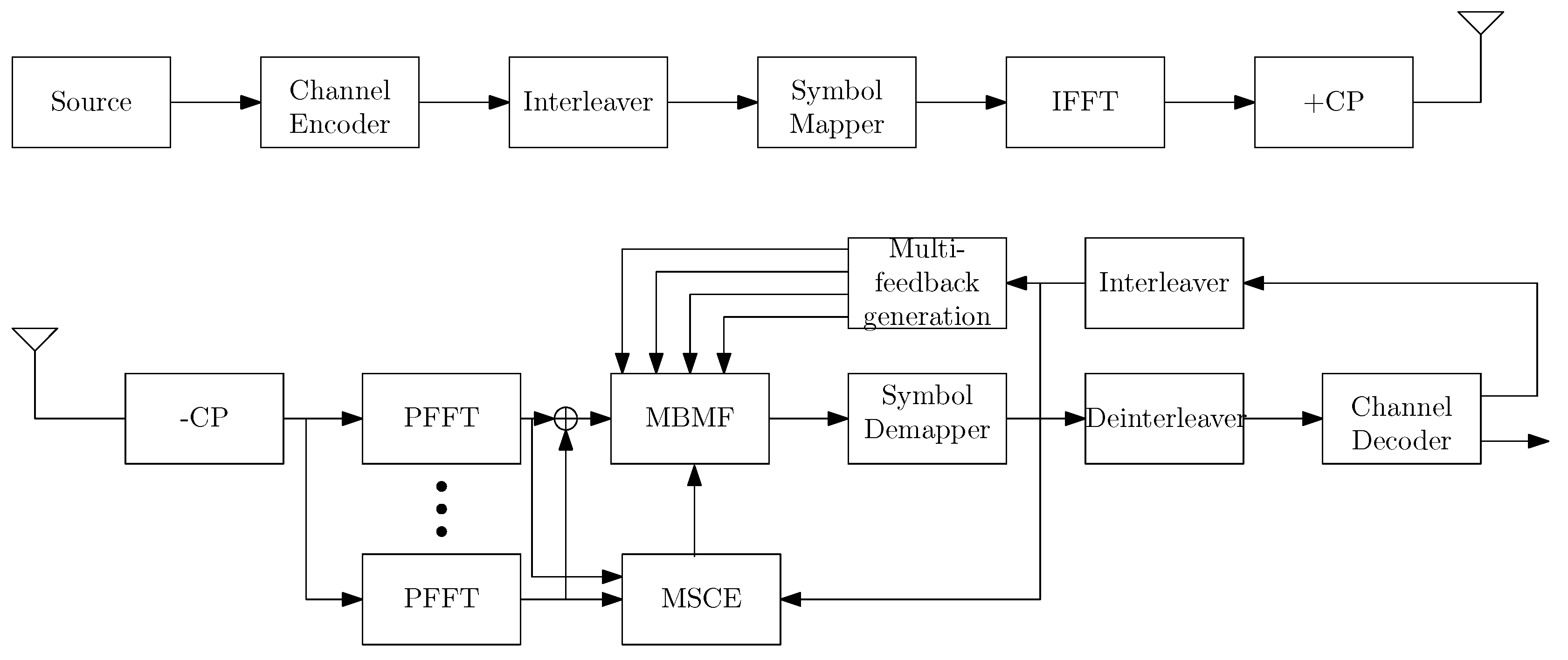
We consider a coded OFDM system with
subcarriers and iterative processing as illustrated in
Figure 1. For a conventional SIC receiver, the number of feedback candidates is reduced to one in the multi-feedback generation block. The information bits are encoded as
by the channel encoder and then interleaved as
through the random interleaver, where the subscript
m denotes the
m-th bit in the sequence. Each group of
c bits is modulated by the symbol mapper onto one symbol
on the
k-th subcarrier at the
i-th OFDM symbol, and then, the inverse fast Fourier transform (IFFT) is performed to obtain the serial data stream. Hence, the signals can be written as:
where the quantity
is transmitted over a time-varying multi-path channel. The cyclic-prefix (CP) is inserted after Equation (
1). Once the distorted transmitted signals reach the receiver, the CP is removed. Then, the received signals during the
i-th OFDM symbol are represented as:
where the quantity
denotes one sample of additive white Gaussian noise (AWGN). The received signals are split into several segments, which go through the PFFT for channel estimation. The summation of the outputs of PFFT blocks is the same as the conventional FFT. Thus, the output is used for equalization as used in conventional OFDM systems. We assume that the
k-th subcarrier is the desired one and omit the noise for simplicity. Substituting Equation (
1) into Equation (
2), Equation (
2) after FFT becomes [
4]:
where
, and the quantity
denotes the channel impulse response for the
n-th time index in one OFDM symbol and the
l-th channel path. If we let
and
,
. As described in [
4], the quantities
d and
k in
can be interpreted as the “Doppler” index and the subcarrier index, respectively. We can also rewrite Equation (
3) in a matrix form:
where the matrix
is illustrated as a circulant matrix in the time domain, and
,
,
,
. The symbol
denotes the matrix with the size of
n by
n.
The matrix
denotes the equivalent frequency channel matrix with the size of
. The output of MBMF block is the output of the equalizer, which yields the estimated symbols
. The bit LLRs corresponding to these symbols can be obtained and deinterleaved for the channel decoder using the MAP algorithm [
25]. The output of the channel decoder, after the interleaver, is also used for the interference cancellation. The interference is regenerated by the multi-feedback generation block. For the conventional SIC receiver, the number of feedback candidates is reduced to one in the output of the multi-feedback generation block. In the following, the processing is based on the frequency domain, unless otherwise specified.
Figure 1.
System model of multiple feedback matched filter (MBMF)-successive interference cancellation (SIC) incorporating multi-segment channel estimation (MSCE).
Figure 1.
System model of multiple feedback matched filter (MBMF)-successive interference cancellation (SIC) incorporating multi-segment channel estimation (MSCE).
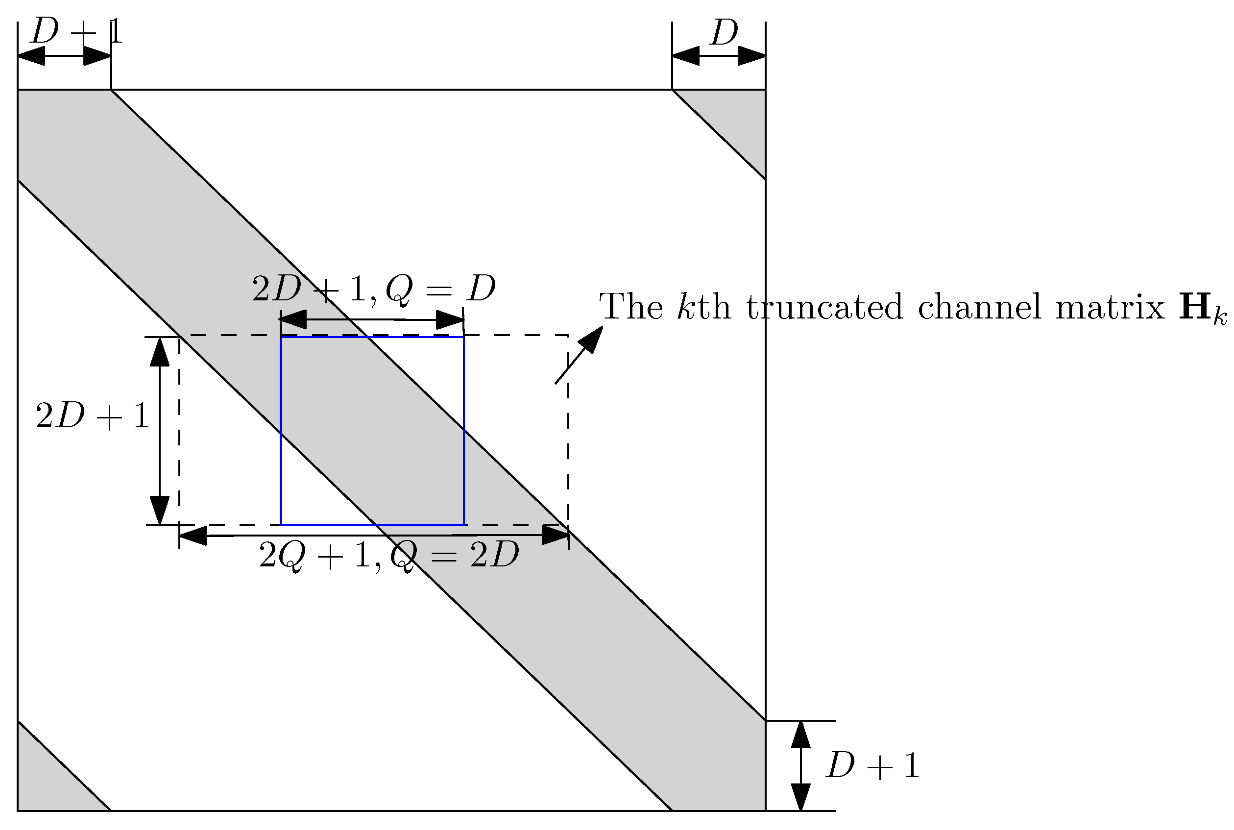
We employ a banded channel matrix
for OFDM systems over doubly-selective channels, as shown in
Figure 2 and [
4], so the truncated system model for the
k-th subcarrier can be approximated as below:
where the truncated received signal is given by
,
denotes the
k-th column vector of the truncated channel matrix, the truncated transmit symbol vector for the
k-th subcarrier is
, the truncated noise vector is expressed by
and the truncated channel matrix
has a size
, as illustrated in
Figure 2.
Figure 2.
The matrix representations of the banded channel matrix , the k-th truncated channel matrix and the reduced channel matrix in the blue square.
Figure 2.
The matrix representations of the banded channel matrix , the k-th truncated channel matrix and the reduced channel matrix in the blue square.
3. Matched Filter Parallel Interference Cancellation
In this section, we present a MF-PIC approach to mitigate the ICI in OFDM systems. The banded structure is employed to reduce the complexity of MF-PIC in the matched filtering stage and the cancellation stage. This is because the elements of
outside the shaded area are omitted for complexity reduction. The LLR calculation of MF-PIC is also discussed as follows. The ICI terms are mostly contributed by
adjacent subcarriers, as illustrated in
Figure 2 and reported in [
4]. Hence, the residual ICI outside the band is considered as noise. The matched filtered signals are expressed as follows:
where the vector
represents the MF outputs. We consider the quadrature phase shift keying (QPSK) here to simplify the exposition, even though we remark that it is straightforward to generalize the LLR processing to other constellations. Hence, the LLR values of
for the channel decoder and the soft symbol estimates for iterative interference cancellation can be computed as [
16]:
Accordingly,
, where the quantity
denotes the
i-th bit of the symbol
at the
k-th subcarrier, and
, because QPSK symbols carry two information bits. Subsequently,
from Equation (
7) is deinterleaved and then fed to the channel decoder as the
a priori LLRs. The extrinsic LLRs of
can be obtained from the channel decoder, and then, the soft symbol estimates
are fed back for soft interference cancellation after the interleaver, as given in Equation (
8). The received data vector after cancellation is given by:
where
,
is the matrix with zero diagonal elements, and the new LLR value
can be re-computed in Equation (
7) to replace
by
. According to Bayes's theorem [
26] and Equation (
7), the soft symbol estimate of the
k-th subcarrier for interference cancellation is given by:
where
. Therefore, the MF-PIC can cancel the ICI in one shot once the
a priori LLR from the channel decoder is known and then fed the new LLR after the ICI cancellation to the channel decoder.
6. BER Analysis of OFDM Systems with Residual ICI
First, the system model in Equation (
2) needs to be rewritten in the following form without the ICI presence for the
l-th path of the time-varying channels:
where
, the random variable (r.v.)
is the random channel gain for the
l-th path at the
n-th time slot, which follows the Rayleigh fading with the zero mean value and the variance
, and
. The AWGN
denotes the same channel. Note that we assume that the interference inside the band is perfectly eliminated by the MBMF canceling strategy for simplicity. The received signal for the
k-th subcarrier can be given as:
where
, and thus, the output signals of the match filter for the decision variable can be given by:
From the equation above, we can observe that the PDF of the SINR becomes very non-trivial due to the superposition of desired signals and ICI from multiple subcarriers. If the channels vary rapidly in the time domain and the number of subcarriers becomes very large, the power of the desired signal (
) from the adjacent subcarrier will become very close to that from the center subcarrier (
) [
4]. Thus, it is possible to approximate Equation (
39) in another form:
To obtain the PDF of the SINR with the aid of Equations (
32) and (
33), the mathematical expression of SINR can be written as [
29]:
where:
In order to further simplify the analysis, the normalized Doppler frequencies and the power are the same for any channel tap. The quantity
is a constant for any
l. The Equation (
41) becomes:
According to [
30], the PDF of
can be expressed as:
where
, and the quantity
denotes the variance of
. We define
,
and
. Additionally, Equation (
43) is rewritten as:
Hence, the PDF of the SINR
ξ can be expressed as [
30]:
For the BER analysis of binary phase shift keying (BPSK) modulation, the conditional BER given the SINR
ξ is given by [
31]:
where the notation
denotes the Q-function for the error probability calculation. The average BER can be given as:
For the numerical evaluation of Equation (
50), the average BER needs to be decomposed as follows:
where
as in [
32]. According to [
29], we can obtain thefollowing equation:
where:
and
denotes the Gamma function. Hence, the average BER can be obtained by Equation (
50) with Equations (
52) and (
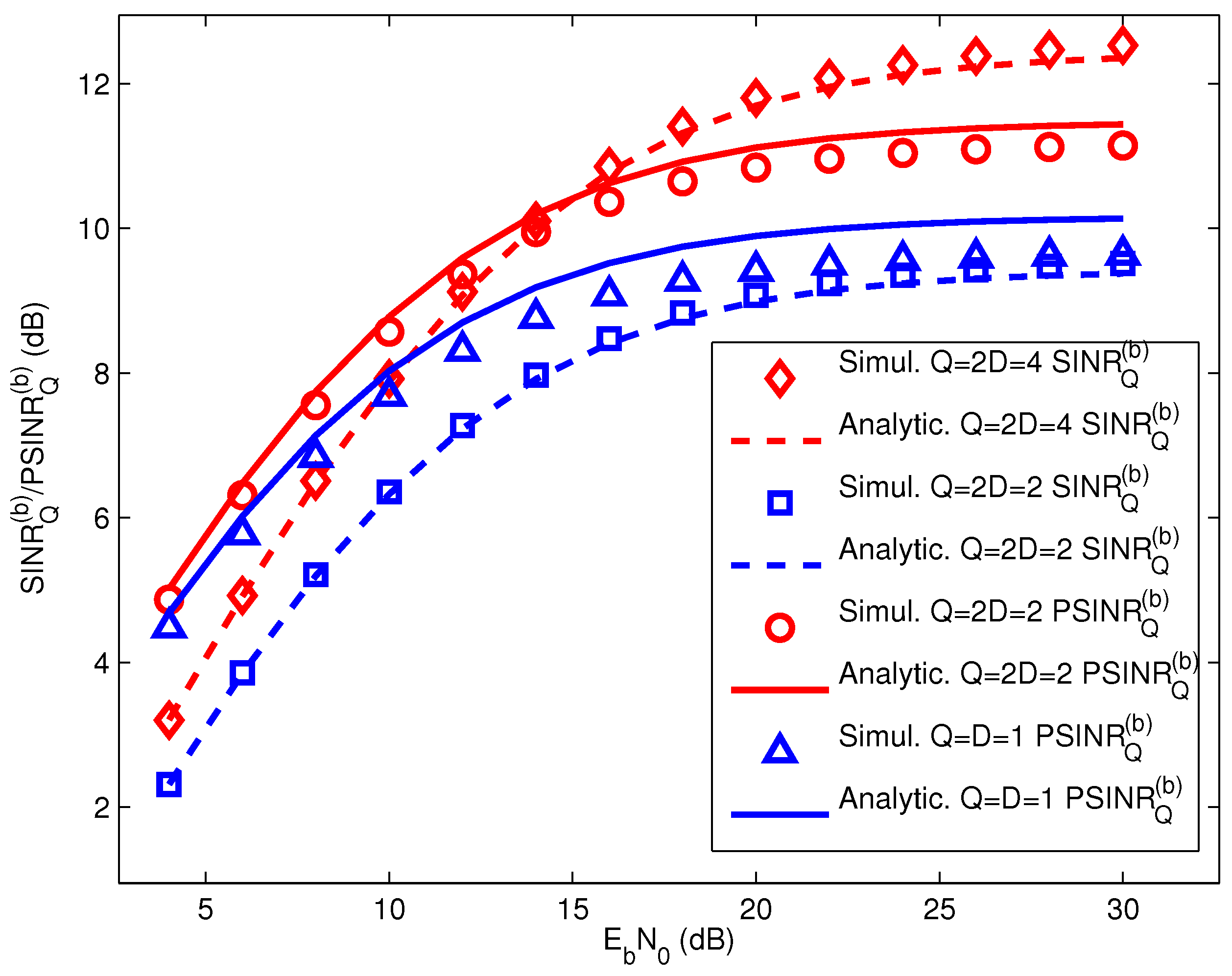
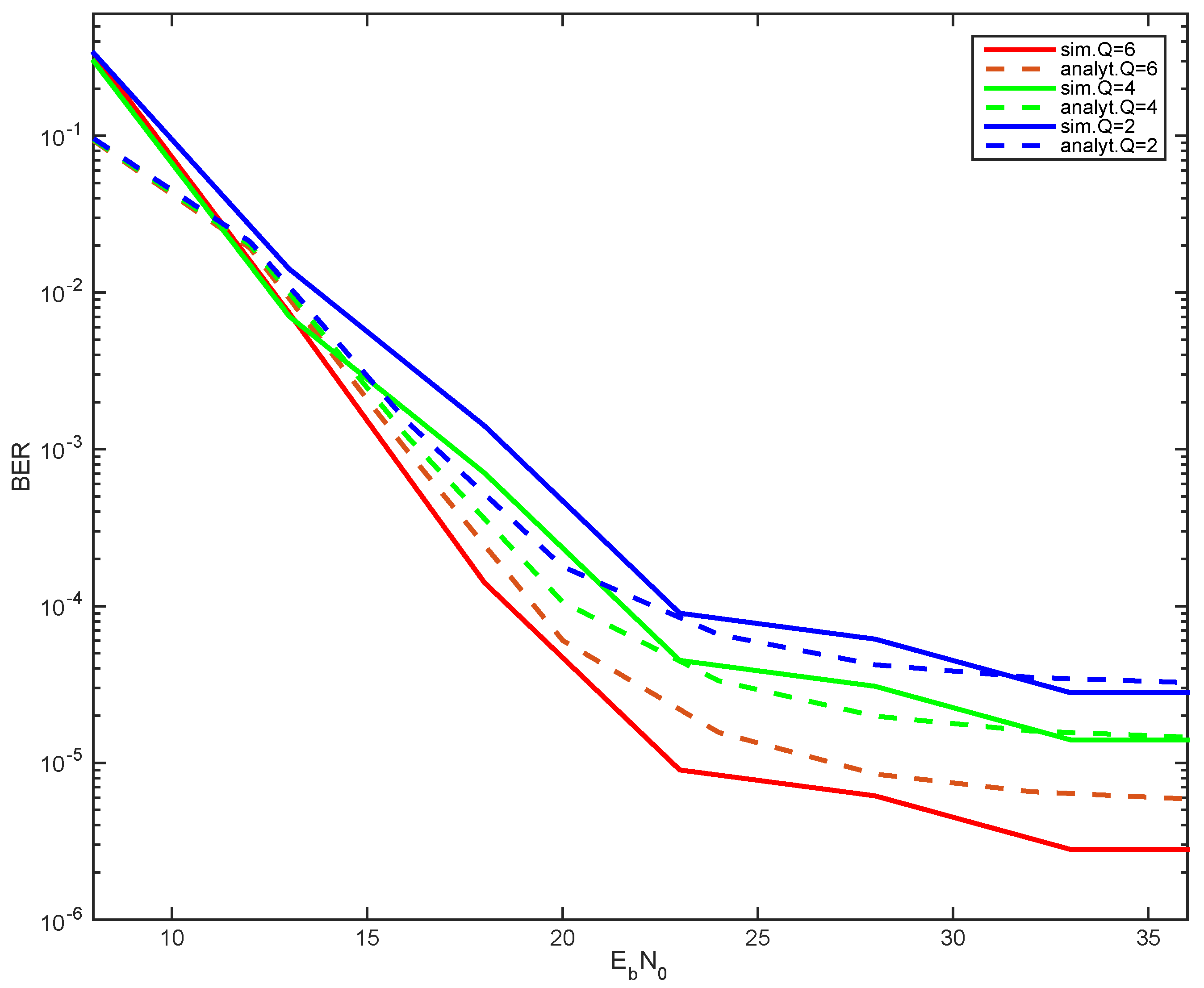
53). The analytical result of the uncoded BER with different band widths
is plotted in
Figure 4, with
the uniform power delay profile
(
is a constant for any
l). It can be observed that the analytical curves are approximately in agreement with the simulated ones, but the curves with
are not plotted due to the significant mismatch to the simulated ones. This is because more interference is removed from the desired signals that cause the inaccuracy of the autocorrelation function of the ICI approximation in Equation (
42), the PDF of which does not follow the similar distribution as described in Equation (
44). Although the mismatch exists in the analysis, the analysis will be more reliable in the low Doppler frequency scenarios with small band sizes
Q.
7. SINR Ordering for MBMF-SIC
For conventional sequential ICI cancellation for OFDM systems, the cancellation is performed on a subcarrier by subcarrier basis, because the previous soft symbol estimates
inside the band are needed in the cancellation for the desired subcarrier
. In this case, there is no significant benefit from the ordering, due to the absence of previous soft symbol estimates. With the iterative ICI cancellation and the channel decoder, the soft symbol estimates
are known beyond the initial iteration, so any ordering can be performed. However, its performance improvement by ordering is very small. On the other hand, the sequential ICI cancellation will introduce the aggregation of residual interference. For MBMF-SIC, the interference is reconstructed by the multi-feedback symbols vectors
, so the aggregation of residual interference from previous soft symbols can be significantly removed. Furthermore, we assume that the conditional probabilities of
given
and
given
are conditionally independent in Equation (
15). This will be true if the residual interference inside the band in Equations (
10) and (
12) dominates. This assumption may be more reasonable by the ordering, which can reduce the coupling effects brought by the previous soft symbol estimates. Following Equations (
10) and (
30), the SINR of the
k-th subcarrier for ordering can be evaluated as similar to the SINR ordering for the conventional SIC.
where
. In the remaining steps, the quantity
can be sorted for
, and the detection ordering can be implemented accordingly. Other ordering methods can also be employed on the basis of the error probability or LLRs, the calculation of which will introduce the channel matrix inversion, with complexity at least
. Hence, the complexity of LLR ordering in [
33] will be more complicated than that of SINR ordering.
Figure 4.
The uncoded bit error rate analysis of the system with the presence of the residual inter-carrier interference (ICI) outside the band (Q = 2,4,6). Ns =128, fdTOFDM = 0.65, .
Figure 4.
The uncoded bit error rate analysis of the system with the presence of the residual inter-carrier interference (ICI) outside the band (Q = 2,4,6). Ns =128, fdTOFDM = 0.65, .
9. Complexity Requirements of MBMF-SIC and MSCE
The complexity of the MBMF-SIC discussed in this chapter is determined by the following parameters: the number of multi-feedback candidates
B, the reduced size truncated channel matrix
, the number of subcarriers
and the number of iterations for the cancellation
P. Following the description of the algorithm in Algorithm 1 with QPSK, the computation of the algorithm for the initial iteration is slightly different from that for the later iterations. However, the computational complexity of the initial iteration is almost identical to that of the later iterations. This is because the initial LLRs first need to be calculated by the output of the matched filter, rather than the direct use of the output of the channel decoder. The computational complexity comes from two aspects: (1) the multi-feedback generation; and (2) the multi-feedback cancellation. The computation of feedback symbols generation for
in Step 11 requires a maximum of
complex additions (CAs) for GSG and TSG, and the computation of the cancellation in Steps 12 and 13 for
requires
complex multiplications (CMs) and
CAs. In Step 14, the computation of average probability of
and the corresponding LLR leads to
CAs. Hence, the total number of complex operations for one iteration required by the MFMB-SIC is
, and the SINR ordering requires a total of
complex operations [
14]. The complexity comparison of ICI cancellation techniques has been made in
Table 1. The complexity of MBMF-SIC and MF-PIC is moderate compared to MF-SIC and much lower than that of conventional MMSE-SIC and banded MMSE-SIC.
Furthermore, the MSCE requires a maximum of
complex operations for each OFDM symbol in the
p-th iteration. This is because the size of the matrix inversion used in Equation (
60) is only related to the number of channel paths
L. The complexity comparison between different channel estimation techniques for rapidly time-varying channels is presented in
Table 2. Note that pilot-assisted LS denotes the pilot-assisted LS channel estimation, which uses the discrete Karhuen–Loève basis expansion model (BEM) to approximate the time-varying channels with the limited number of expansion coefficients [
36]. The number of expansion coefficients is lower bounded by
as described in [
35]. The significant advantage of MSCE over the method in [
36] is the use of linear interpolation to approximate the channels between two segments in the OFDM symbol. Hence, the MSCE can be considered as a special representation of BEM with two expansion coefficients. Compared to SBCE, the complexity of MSCE is a bit higher; because the matrix inversion with the size
L is required to estimate the channels in the mid-point of each segment.
Table 1.
Complexity comparison between different interference cancellation techniques for the p-th iteration. BP, belief propagation; RSL, recursive-SIC-linear-MMSE.
Table 1.
Complexity comparison between different interference cancellation techniques for the p-th iteration. BP, belief propagation; RSL, recursive-SIC-linear-MMSE.
| Algorithm | Complex Operations |
|---|
| MMSE-SIC [37] | |
| banded MMSE-SIC [4] | |
| MF-SIC [16] | |
| MF-PIC [17] | |
| RSL [3] | |
| BP-MAP [15] | * denotes the number of constellation points |
| MBMF-SIC | |
| MBMF-SIC + SINR ordering | |
Table 2.
Complexity comparison between different channel estimation techniques for the p-th iteration.
Table 2.
Complexity comparison between different channel estimation techniques for the p-th iteration.
| Algorithm | Complex Operations |
|---|
| SBCE [16] | |
| PA-LS [36] | |
| MSCE | |
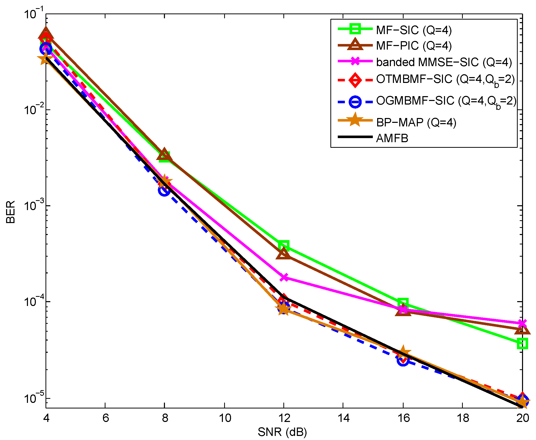
Figure 5.
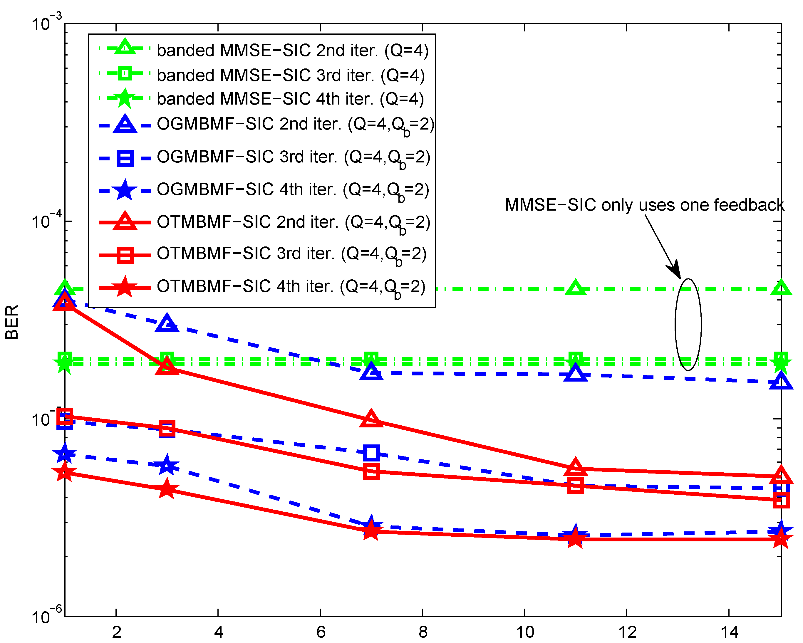
BER performance against SNR (dB) of MF-PIC, GSG-based MBMF-SIC, ordering GSG-based MBMF (OGMBMF)-SIC, TSG-based MBMF (TMBMF)-SIC, ordering TMBMF (OTMBMF)-SIC, MF-SIC, banded MMSE-SIC and approximate matched filter bound (AMFB) in the fourth iteration with .
Figure 5.
BER performance against SNR (dB) of MF-PIC, GSG-based MBMF-SIC, ordering GSG-based MBMF (OGMBMF)-SIC, TSG-based MBMF (TMBMF)-SIC, ordering TMBMF (OTMBMF)-SIC, MF-SIC, banded MMSE-SIC and approximate matched filter bound (AMFB) in the fourth iteration with .
10. Simulation Results
In this section, the performance of the proposed methods (MF-PIC and MBMF-SIC) will be evaluated in terms of BER in different scenarios. We assume a scenario with the following settings: the carrier frequency
; the subcarrier spacing
; and the OFDM symbol period is
. The number of subcarriers is
. The symbols are modulated by QPSK, the extension of which to other modulation schemes is straightforward. In addition, a
rate convolutional code with generator polynomial
is employed for the iterative interference cancellation, and the length of the code is 2560 bits. A wide-sense stationary uncorrelated scattering channel with a uniform power delay profile is simulated according to the Jakes model and the normalized Doppler frequency
. The maximum delay of the channel is
. Because of the band assumption, we assume
as described in [
4,
5] given the time-domain window. For MSCE, the number of segments
is used, and the number of pilots
. We also define an approximate matched filter bound (AMFB) [
4] as a benchmark for ICI cancellation, which implies that the ICI inside the band
is perfectly removed. Additionally, we use the banded MMSE-SIC [
4], MF-SIC [
16] and MBMF-SIC with and without SINR ordering, as well as AMFB for comparison.
In
Figure 5, we introduce several OFDM equalization techniques for comparison. The list includes the approximate MAP equalizers, namely belief propagation Ungerboeck-MAP (BP-MAP), recursive-SIC-linear-MMSE (RSL) in [
3,
15], the benchmark AMFB without ICI inside the band [
2], the banded MMSE-SIC [
4] and MF-SIC [
16]. Note that the RSL we used is a modified SIC-MMSE with two taps (
) in the fourth iteration. The BER performance of GSG-based MBMF-SIC (GMBMF-SIC) and TSG-based MBMF-SIC (TMBMF-SIC) with SINR ordering show performances close to the approximate MAP equalizers (BP-MAP), with only 1 dB loss with the BP-MAP and a fraction of 1 dB loss with the benchmark AMFB. The proposed scheme may significantly reduces the error floor compared to banded MMSE-SIC and MBMF-SIC without SINR ordering. It can be seen that the SINR ordering improves the reliability of detected symbols and makes the assumption for Equation (
14) more appropriate. For a fair comparison, the SINR ordering in
Section 7 is incorporated in other schemes in the later, iterations except for the first iteration. This is because serial ICI cancellation requires previous symbol estimates to improve the reliability of the remaining symbols. However, the ordering for MBMF-SIC can be employed in the initial iteration due to the use of LLR to generate multi-feedback candidates in the Steps 3 and 4 of Algoritm 1. We can also observe that the BER performance difference between GMBMF-SIC and TMBMF-SIC is negligible, but TSG performs better than GSG. This also agrees with the statements in [
27] that the tree search algorithm works better than the Gibbs sampler at high SNR. For simplicity, we only consider GMBMF-SIC and TMBMF-SIC with SINR ordering in the rest of the chapter, which will be referred to as OGMBMF-SIC and OTMBMF-SIC. Furthermore, the curves of OTMBMF-SIC may not be shown in some following figures, because there is no significant difference between OGMBMF-SIC and OTMBMF-SIC in the BER performance. In what follows, the RSL is not plotted, due to its close to AMFB performance. Unlike the RSL, the BP-MAP may outperform other ICI cancellation methods. This is because the ICI cancelers mitigate the uncoded interference from neighbor subcarriers, but in the BP-MAP scheme, more reliable extrinsic information is obtained from the channel decoder in an iterative detection and decoding system. Hence, its performance will be improved by the additional weights when the LLR value is updated. However, the BP-MAP performs a little worse than the proposed MBMF-SIC with SINR ordering, which introduces additional precoding gain and removes the error floor.
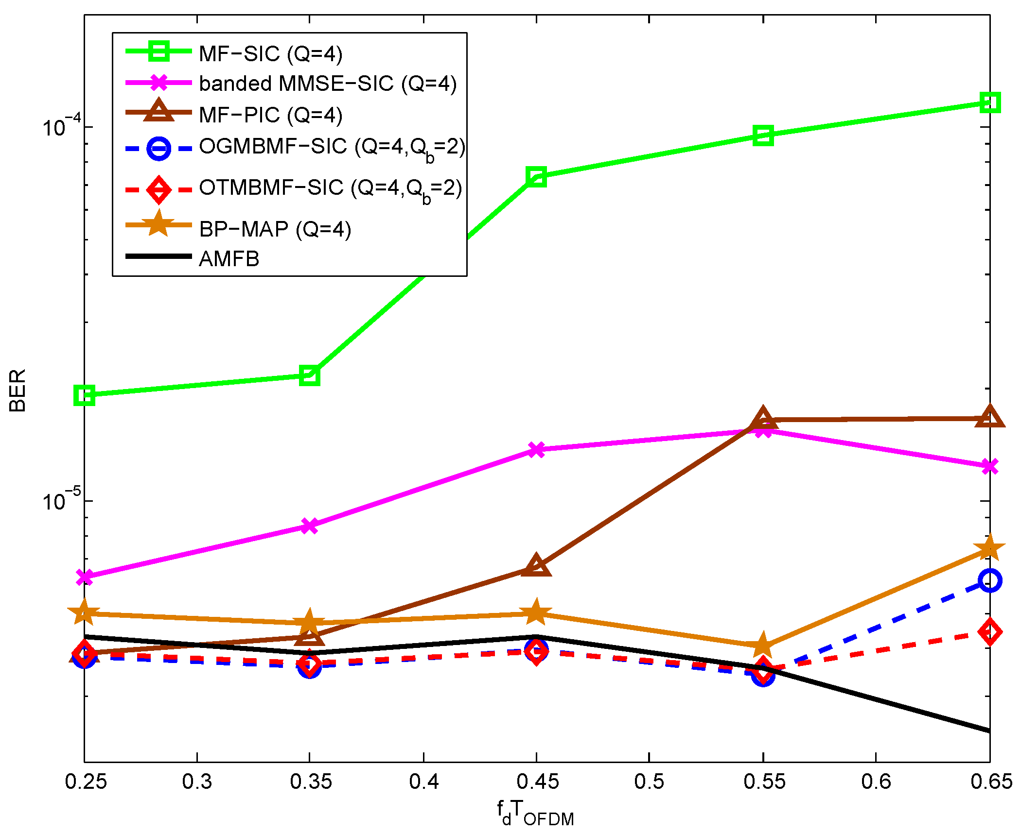
The BER performance of the fourth iteration against normalized Doppler frequencies
from
to
has been illustrated in
Figure 6, which validates the statements that the proposed OGMBMF-SIC and OTMBMF-SIC can work in a wide range of high Doppler frequencies
. We can observe that the power of ICI inside the band is reduced at high Doppler frequencies. Additionally, the MF-SIC and MF-PIC can only be used at low Doppler frequencies.
Figure
Figure 7 compares the BER performance against SNR (dB) with a normalized Doppler frequency
in the fourth iteration. The MSCE is iteratively performed in every iteration, once the new symbol estimates become available from the channel decoder. The BER performance of these receivers in the first iteration is very poor, with
, which may not be useful for comparison. Matched filter-based receivers (MF-SIC, OGMBMF-SIC) are less sensitive to channel estimation errors, because they do not make use of channel coefficients as much as banded MMSE-SIC. For banded MMSE-SIC, the autocorrelation matrix must be used, which may amplify the channel estimation errors. In
Figure 5, the banded MMSE-SIC outperforms MF-SIC with perfect channel knowledge in the BER performance. However, their performance at SNR
dB has been degraded to the same level of BER (less than 1 dB performance loss) in the fourth iteration with MSCE. MF-PIC is not very close to banded MMSE-SIC with channel estimation, because the autocorrelation matrix is also required for MF-PIC for ICI cancellation. Intuitively, the proposed OGMBMF-SIC has the same advantages as MF-SIC. With MSCE, OGMBMF-SIC can still achieve an acceptable BER performance in such a high mobility scenario (
), which makes OGMBMF-SIC more practical.
Figure 6.
BER performance against of MF-PIC, OGMBMF-SIC, OTMBMF-SIC, MF-SIC and banded MMSE-SIC in the fourth iteration at SNR =12 dB.
Figure 6.
BER performance against of MF-PIC, OGMBMF-SIC, OTMBMF-SIC, MF-SIC and banded MMSE-SIC in the fourth iteration at SNR =12 dB.
Figure 7.
BER performance against SNR (dB) of MF-PIC, GMBMF-SIC, OGMBMF-SIC, MF-SIC, banded MMSE-SIC and AMFB using MSCE in the fourth iteration with fdTOFDM = 0.65.
Figure 7.
BER performance against SNR (dB) of MF-PIC, GMBMF-SIC, OGMBMF-SIC, MF-SIC, banded MMSE-SIC and AMFB using MSCE in the fourth iteration with fdTOFDM = 0.65.
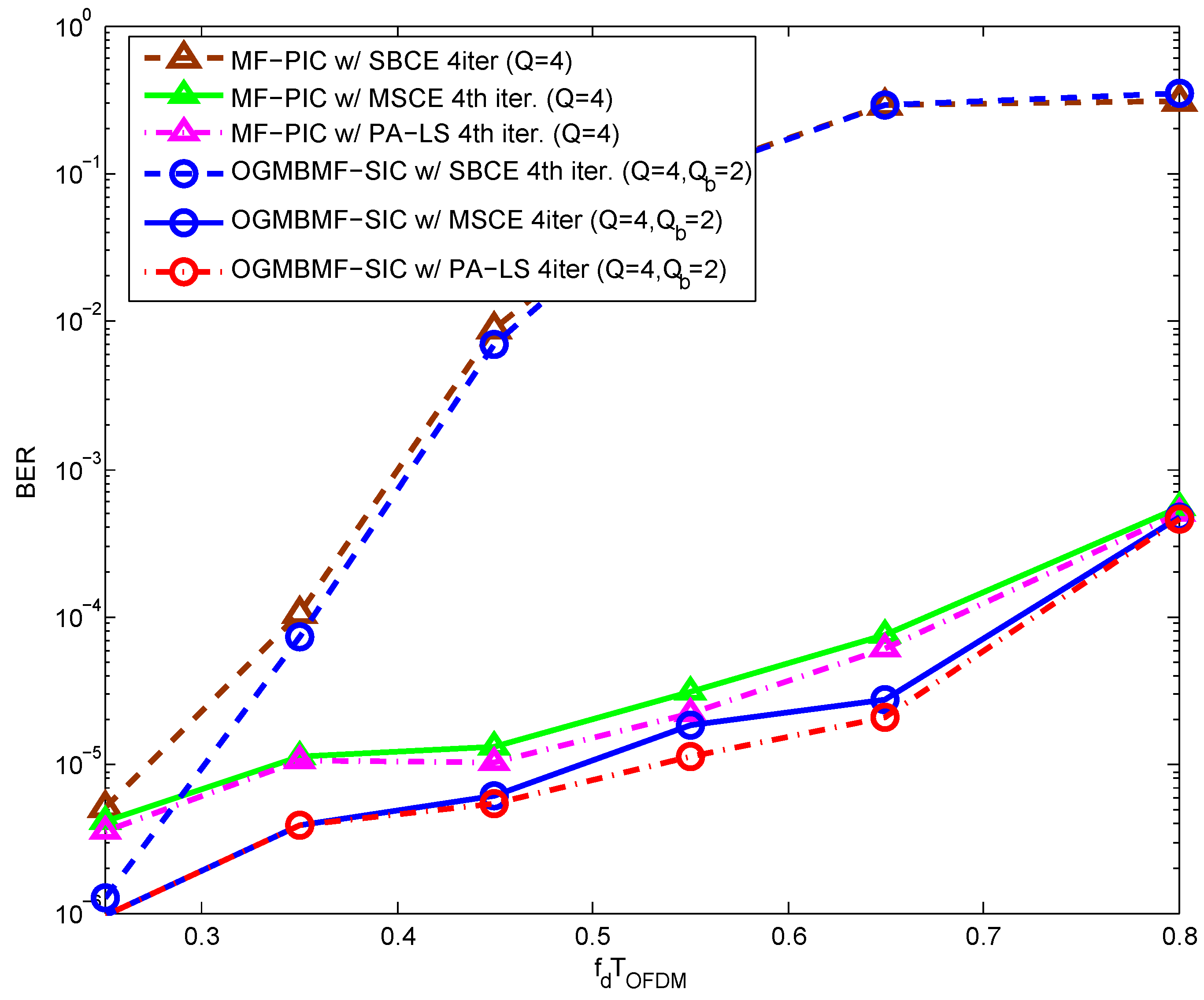
To show the robustness to the high normalized Doppler frequencies, we compared the SBCE, PA-LS and MSCE in terms of BER performance in the fourth iteration. In
Figure 8, the MF-PIC and OGMBMF-SIC with SBCE cannot work at normalized Doppler frequencies over
. Additionally, the curves for MSCE are almost identical to those for PA-LS, only slightly poorer at high normalized Doppler frequencies, which implies that the MSCE performed in an iterative manner and with the aid of data symbols can approach the performance of PA-LS, which uses the discrete Karhunen-Loève (DKL)-basis expansion model (BEM) to approximate the channels with five expansion coefficients.
Figure 8.
BER performance against of OGMBMF-SIC and MF-PIC using MSCE and single-burst channel estimation (SBCE) in the fourth iteration at SNR =16 dB.
Figure 8.
BER performance against of OGMBMF-SIC and MF-PIC using MSCE and single-burst channel estimation (SBCE) in the fourth iteration at SNR =16 dB.
To determine an appropriate number of multi-feedback candidates (
B) of MBMF-SIC for a given normalized Doppler frequency, the BER performance against the number of feedback elements has been plotted in
Figure 9 for OGMBMF-SIC and OTMBMF-SIC. The BER performance improves with an increasing number of feedback elements. We also observed that both of them reach the optimum BER performance around
in the fourth iteration, which implies that both generation mechanisms can be considered as equivalent, if more iterations are performed by the receivers. Unlike the BER performance of OTMBMF-SIC, the BER performance of OGMBMF-SIC is poorer than that of OTMBMF-SIC in the first several iterations. This is because the feedback of OGMBMF-SIC is randomly generated given the
a priori probability from the output of the channel decoder, and we assume each of them has equal probability, which may introduce instability into the LLR calculation with the increasing number of feedback elements. For OTMBMF-SIC, each feedback candidate has been weighted given the probability, so the feedback elements with low probability will not have a significant influence on the BER performance. In other words, it only takes the most significant feedback candidates into account. Furthermore, MBMF-SIC is not equivalent to the MAP algorithm and employs the reduced channel matrix in the multi-feedback cancellation. Thus, a large
B does not significantly improve the BER performance as compared to a small
B.
Figure 9.
BER performance against the number of multi-feedback candidates B with at SNR =12 dB.
Figure 9.
BER performance against the number of multi-feedback candidates B with at SNR =12 dB.


