
Robust Rank Reduction Algorithm with Iterative Parameter Optimization and Vector Perturbation

Abstract
:1. Introduction
- A bank of perturbed steering vectors is proposed as candidate array steering vectors around the true steering vector. The candidate steering vectors are responsible for performing rank reduction, and the reduced-rank beamformer forms the beam in the direction of the signal of interest (SoI).
- We devise efficient stochastic gradient (SG) and recursive least-squares (RLS) algorithms for implementing the proposed robust IOVP design.
- We introduce an automatic rank selection scheme in order to obtain the optimal beamforming performance with low computational complexity.
2. System Model
2.1. Minimum Variance Distortionless Response
2.2. Recursive Least-Squares
3. Problem Statement and the Dimension Reduction with IOVP
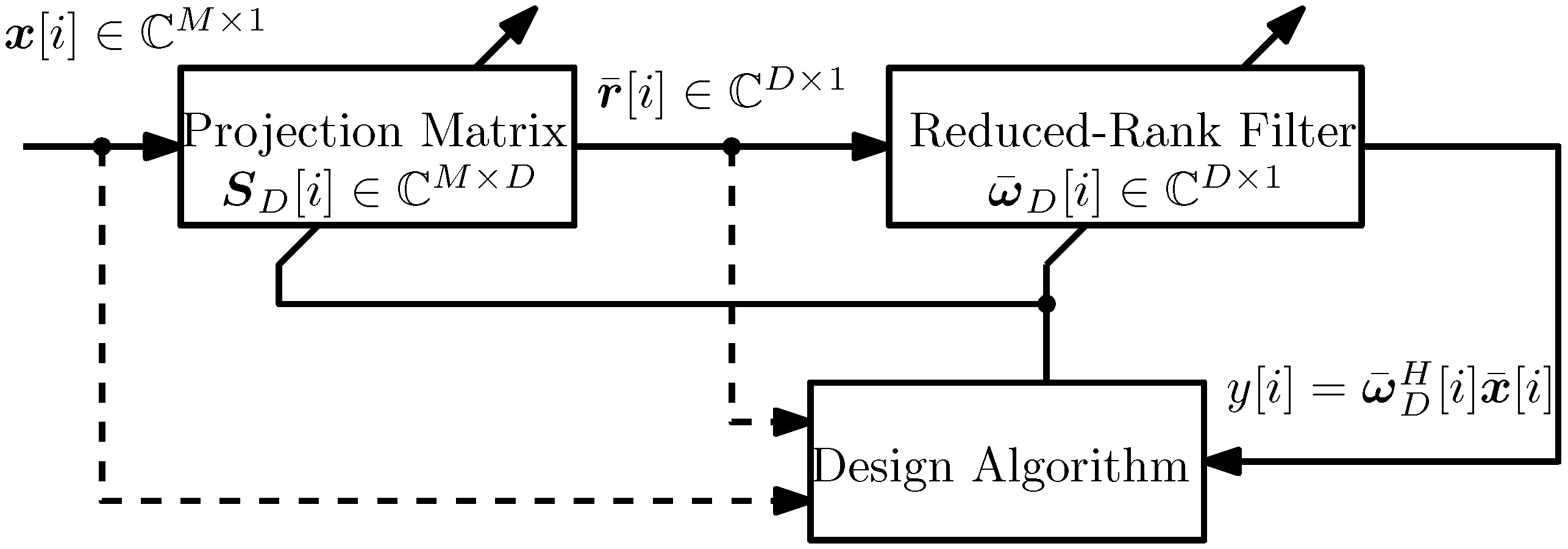
3.1. Reduced Rank Methods and the Projection Matrix
3.2. Problem Statement and the Proposed IOVP

3.3. Stochastic Gradient Adaptation
3.4. Recursive Least-Squares Adaptation
4. Proposed Robust Capon IOVP Beamforming
4.1. Stochastic Gradient Adaptation
4.2. Recursive Least-Squares Adaptation
5. Rank Selection
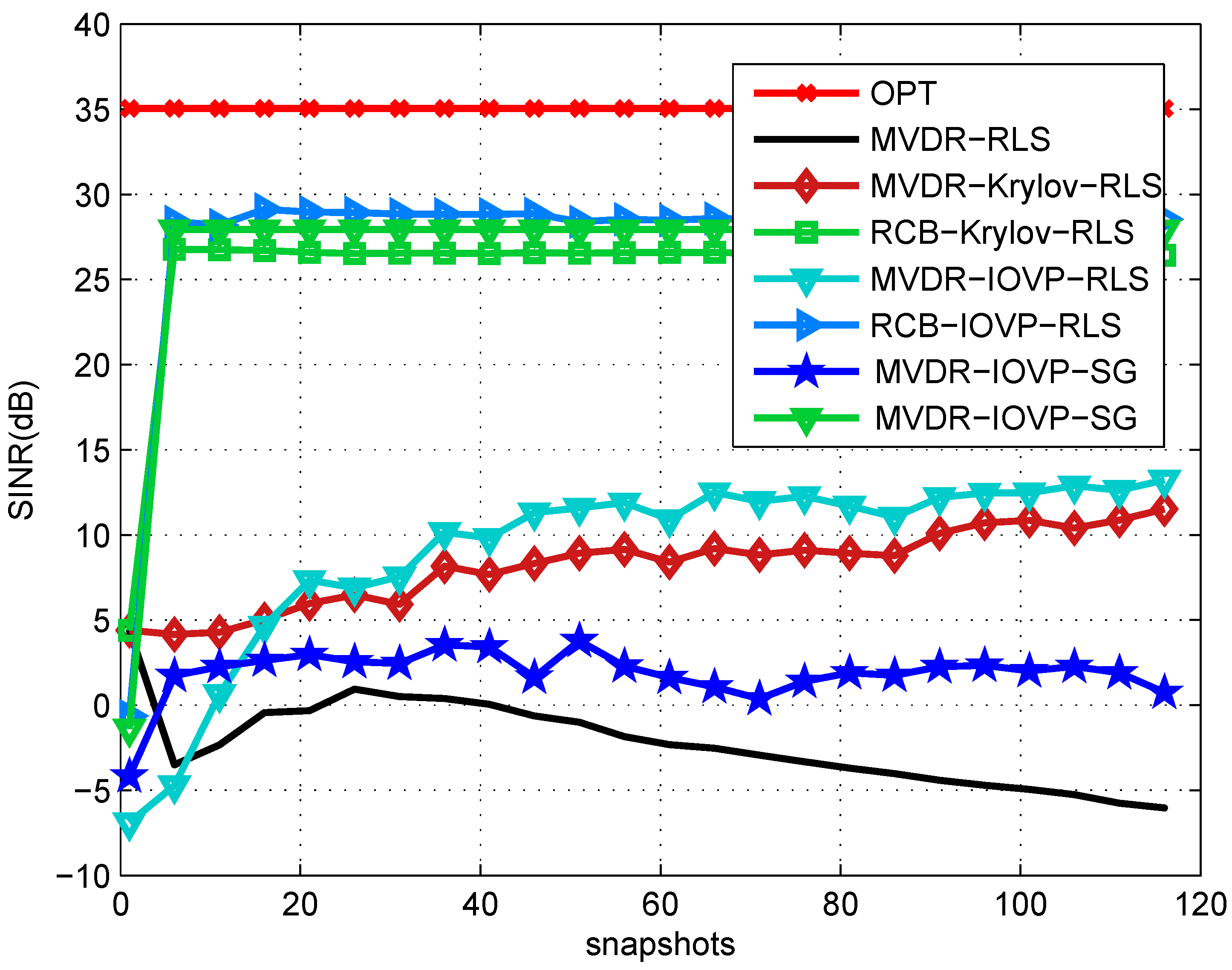
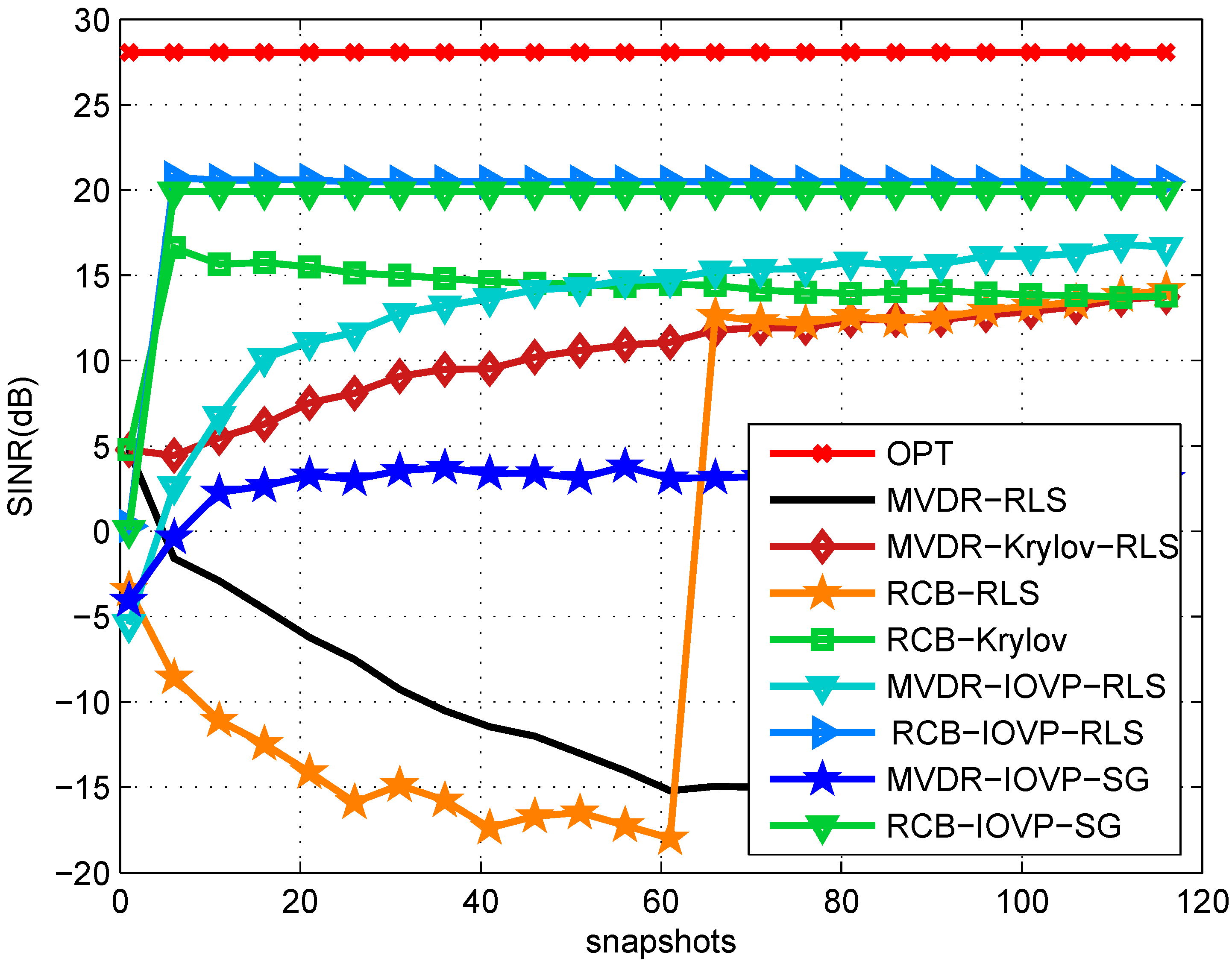
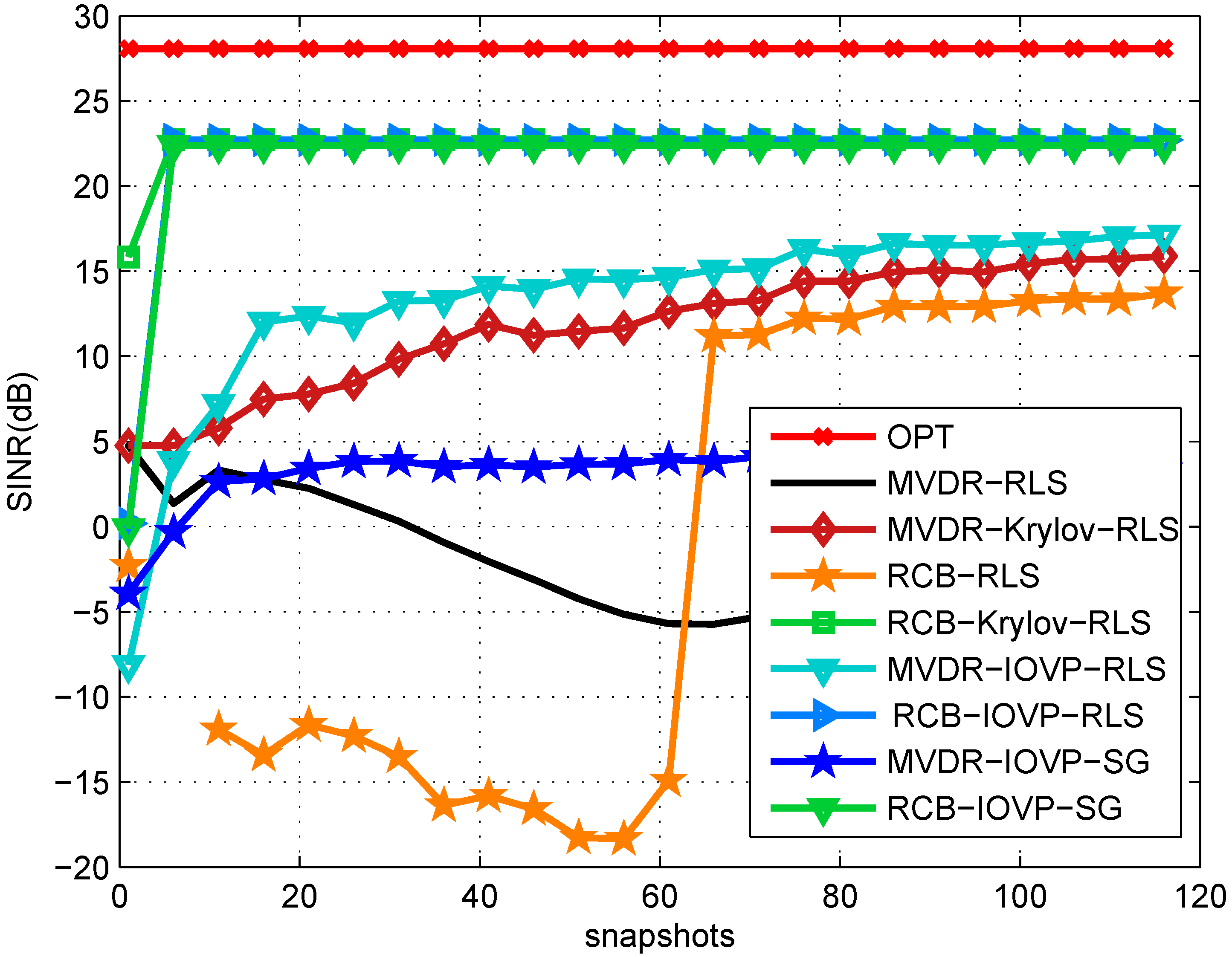
6. Simulations

| Snapshots | Signal 1 (SoI) | Signal 2 | Signal 3 | Signal 4 |
|---|---|---|---|---|
| 1 to 120 | 10/90 | 20/35 | 20/135 | 20/165 |

7. Conclusions
Acknowledgements
Author Contributions
Conflicts of Interest
References
- Van Trees, H. L. Detection, Estimation, and Modulation Theory, Part IV, Optimum Array Processing; John Wiley & Sons: Hoboken, NJ, USA, 2002. [Google Scholar]
- Haykin, S. Adaptive Filter Theory; Fourth ed.; Prentice-Hall: Englewood Cliffs, NJ, USA, 2002. [Google Scholar]
- Li, J.; Stoica, P. Robust Adaptive Beamforming; John Wiley & Sons: Hoboken, NJ, USA, 2006. [Google Scholar]
- Li, J.; Stoica, P.; Wang, Z. On Robust Capon Beamforming and Diagonal Loading. IEEE Trans. Signal Process. 2003, 51, 1702–1715. [Google Scholar]
- Scharf, L. L.; Tufts, D. W. Rank reduction for modeling stationary signals. IEEE Trans. Acoust. Speech Signal Process. 1987, 35, 350–355. [Google Scholar] [CrossRef]
- Vorobyov, S. A.; Gershman, A. B.; Luo, Z.-Q. Robust Adaptive Beamforming Using Worst-Case Performance Optimization: A Solution to the Signal Mismatch Problem. IEEE Trans. Signal Process. 2003, 51, 313–324. [Google Scholar] [CrossRef]
- Somasundaram, S. D. Reduced Dimension Robust Capon Beamforming for Large Aperture Passive Sonar Arrays. IET Radar Sonar Navig. 2011, 5, 707–715. [Google Scholar] [CrossRef]
- Scharf, L. L.; van Veen, B. Low rank detectors for Gaussian random vectors. IEEE Trans. Acoust. Speech Signal Process. 1987, 35, 1579–1582. [Google Scholar] [CrossRef]
- Burykh, S.; Abed-Meraim, K. Reduced-rank adaptive filtering using Krylov subspace. EURASIP J. Appl. Signal Process. 2002, 12, 1387–1400. [Google Scholar] [CrossRef]
- Goldstein, J. S.; Reed, I. S.; Scharf, L. L. A multistage representation of the Wiener filter based on orthogonal projections. IEEE Trans. Inf. Theory 1998, 44, 2943–2959. [Google Scholar] [CrossRef]
- Hassanien, A.; Vorobyov, S. A. A Robust Adaptive Dimension Reduction Technique with Application to Array Processing. IEEE Signal Process. Lett. 2009, 16, 22–25. [Google Scholar] [CrossRef]
- Ge, H.; Kirsteins, I. P.; Scharf, L. L. Data Dimension Reduction Using Krylov Subspaces: Making Adaptive Beamformers Robust to Model Order-Determination. In Proceedings of the IEEE International Conference on Acoustics, Speech and Signal Processing, Toulouse, France, 14–19 May 2006; Volume 4, pp. 1001–1004.
- Wang, L.; de Lamare, R. C. Constrained adaptive filtering algorithms based on conjugate gradient techniques for beamforming. IET Signal Process. 2010, 4, 686–697. [Google Scholar] [CrossRef]
- Somasundaram, S.; Li, P.; Parsons, N.; de Lamare, R. C. Data-adaptive reduced-dimension robust Capon beamforming. In Proceedings of the IEEE International Conference on Acoustics, Speech and Signal Processing, Vancouver, BC, Canada, 26–31 May 2013.
- De Lamare, R. C.; Sampaio-Neto, R. Adaptive reduced-rank processing based on joint and iterative interpolation, Decimation and Filtering. IEEE Trans. Signal Process. 2009, 57, 2503–2514. [Google Scholar] [CrossRef]
- De Lamare, R. C.; Wang, L.; Fa, R. Adaptive reduced-rank LCMV beamforming algorithms based on joint iterative optimization of filters: design and analysis. Signal Process. 2010, 90, 640–652. [Google Scholar] [CrossRef]
- Fa, R.; de Lamare, R. C.; Wang, L. Reduced-rank STAP schemes for airborne radar based on switched joint interpolation, decimation and filtering algorithm. IEEE Trans. Signal Process. 2010, 58, 4182–4194. [Google Scholar] [CrossRef]
- Grant, D. E.; Gross, J. H.; Lawrence, M. Z. Cross-spectral matrix estimation effects on adaptive beamformer. J. Acoust. Soc. Am. 1995, 98, 517–524. [Google Scholar] [CrossRef]
- Elnashar, A. Efficient implementation of robust adaptive beamforming based on worst-case performance optimisation. IET Signal Process. 2008, 4, 381–393. [Google Scholar] [CrossRef]
- Honig, M. L.; Goldstein, J. S. Adaptive reduced-rank interference suppression based on the multistage Wiener filter. IEEE Trans. Commun. 2002, 50, 986–994. [Google Scholar] [CrossRef]
- Haoli, Q.; Batalama, S.N. Data record-based criteria for the selection of an auxiliary vector estimator of the MMSE/MVDR filter. IEEE Trans. Commun. 2003, 51, 1700–1708. [Google Scholar] [CrossRef]
© 2015 by the authors; licensee MDPI, Basel, Switzerland. This article is an open access article distributed under the terms and conditions of the Creative Commons Attribution license (http://creativecommons.org/licenses/by/4.0/).
Share and Cite
Li, P.; Feng, J.; De Lamare, R.C. Robust Rank Reduction Algorithm with Iterative Parameter Optimization and Vector Perturbation. Algorithms 2015, 8, 573-589. https://0-doi-org.brum.beds.ac.uk/10.3390/a8030573
Li P, Feng J, De Lamare RC. Robust Rank Reduction Algorithm with Iterative Parameter Optimization and Vector Perturbation. Algorithms. 2015; 8(3):573-589. https://0-doi-org.brum.beds.ac.uk/10.3390/a8030573
Chicago/Turabian StyleLi, Peng, Jiao Feng, and Rodrigo C. De Lamare. 2015. "Robust Rank Reduction Algorithm with Iterative Parameter Optimization and Vector Perturbation" Algorithms 8, no. 3: 573-589. https://0-doi-org.brum.beds.ac.uk/10.3390/a8030573