Article

Gradient-Based Iterative Identification for Wiener Nonlinear Dynamic Systems with Moving Average Noises

School of Electrical and Automatic Engineering, Changshu Institute of Technology, Hushan RoadNo.99, Changshu 215500, China
*
Author to whom correspondence should be addressed.
Algorithms 2015, 8(3), 712-722; https://0-doi-org.brum.beds.ac.uk/10.3390/a8030712
Submission received: 30 June 2015 / Revised: 20 July 2015 / Accepted: 20 August 2015 / Published: 26 August 2015
(This article belongs to the Special Issue Numerical Algorithms for Solving Nonlinear Equations and Systems)

Abstract

:
This paper focuses on the parameter identification problem for Wiener nonlinear dynamic systems with moving average noises. In order to improve the convergence rate, the gradient-based iterative algorithm is presented by replacing the unmeasurable variables with their corresponding iterative estimates, and to compute iteratively the noise estimates based on the obtained parameter estimates. The simulation results show that the proposed algorithm can effectively estimate the parameters of Wiener systems with moving average noises.

1. Introduction

In actual industry processes, block-oriented nonlinear systems are often introduced to model nonlinear systems. Block-oriented nonlinear systems can be commonly divided into Hammerstein systems and Wiener systems [1,2,3]. Hammerstein systems consist of a linear block following a static nonlinear block [4,5,6]. Wiener systems are composed of a linear block preceding a static nonlinear block [7,8,9]. The output of Wiener systems is nonlinear, so the modeling for Wiener systems is more sophisticated than that for Hammerstein systems. Differing from the work in [8,9], this paper focuses on the identification problem for Wiener nonlinear systems with moving average noises which are called Wiener output error moving average (OEMA) systems. In most existing works, the nonlinear part of Wiener systems is assumed a linear combination or a piecewise-linear function [10], or has a invertible and monotone function representation over the operating range [11,12]. Wang and Ding derived a least squares-based and a gradient-based iterative identification algorithms for Wiener nonlinear systems by separating one bilinear cost function into two linear cost functions [13]. Hagenblad et al. presented a maximum likelihood method to identify Wiener models [14].
The stochastic gradient (SG) algorithm has less computational burden and slower convergence rate than the recursive least squares algorithm [15,16,17]. Some new algorithms were presented to improve the convergence rate of the SG algorithm [18,19,20]. For example, Ding et al. introduced the convergence index to the SG algorithm and obtained a faster convergence rate than stochastic gradient algorithm [21]; Liu et al. derived the multi-innovation extended stochastic gradient algorithm for controlled autoregressive moving average models by expanding the scalar innovation to an innovation vector and analyzed its performance in detail [22]. Recently, the gradient-based iterative (GI) algorithm was also presented to improve the convergence rate of the SG algorithm [23,24,25]. By making sufficient use of all the measured information, the GI algorithm can obtain a faster convergence rate than the SG algorithm. Wang et al. presented a gradient-based iterative identification algorithms for Box-Jenkins systems with finite measurement input-output data [26]. Li et al. proposed a gradient based iterative algorithm to determine the parameters of a nonlinear system by using the negative gradient search [27]. Zhang et al. derived a hierarchical gradient based iterative estimation algorithm for multivariable output error moving average systems using the hierarchical identification principle [28].
To the best of our knowledge, few contributions have addressed the modeling and estimation issues for Wiener nonlinear OEMA systems, which are the focus of this work. For Wiener nonlinear OEMA systems, our objectives are as follows:
  • To establish the identification model of the Wiener nonlinear OEMA system from input to output.
  • To present a gradient-based iterative identification algorithm for the Wiener nonlinear OEMA model.
  • To analyze the performances of the proposed algorithm using a numerical simulation, including the convergence rates and the estimation errors of this algorithm.
The rest of this paper is organized as follows. Section 2 establishes the identification model of the Wiener nonlinear OEMA system. Section 3 presents a gradient-based iterative identification algorithm for the Wiener nonlinear OEMA model. Section 4 provides an example to illustrate the effectiveness of the proposed algorithm. The conclusions of the paper are summarized in Section 5.

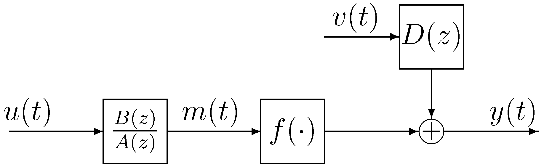
2. The Derivation of the Wiener OEMA Model

Let us firstly introduce some notations. The superscript T denotes the matrix transpose; 1 n represents an n-dimensional column vector whose elements are 1; the norm of a matrix X is defined by X 2 = tr [ X X T ] .
Figure 1. The Wiener nonlinear OEMA system.
Algorithms 08 00712 g001
Consider a Wiener nonlinear OEMA system shown in Figure 1:
m ( t ) = B ( z ) A ( z ) u ( t )
y ( t ) = f ( m ( t ) ) + D ( z ) v ( t )
where u ( t ) is the system input, y ( t ) is the system output and v ( t ) is an additive noise with zero mean; the inner variable m ( t ) (namely, the output of the linear block) is unmeasurable; A ( z ) , B ( z ) and D ( z ) are polynomials in the shift operator z - 1 [ z - 1 y ( t ) = y ( t - 1 ) ] with
A ( z ) : = 1 + a 1 z - 1 + a 2 z - 2 + + a n a z - n a B ( z ) : = b 1 z - 1 + b 2 z - 2 + + b n b z - n b D ( z ) : = 1 + d 1 z - 1 + d 2 z - 2 + + d n d z - n d
The nonlinear part f ( · ) in the Wiener system is a polynomial of a known order as follows:
f ( m ( t ) ) = γ 1 m ( t ) + γ 2 m 2 ( t ) + + γ n γ m n γ ( t )
where n γ is the polynomial orders.
Equation (1) can be rewritten to
m ( t ) = [ 1 - A ( z ) ] m ( t ) + B ( z ) u ( t )
In order to get unique parameter estimates, we introduce the key term separation technique presented in [7,29] and let the first coefficient of the nonlinear part be unity, i.e., γ 1 = 1 . Then, we have
y ( t ) = m ( t ) + i = 2 n γ γ i m i ( t ) + D ( z ) v ( t )
Here m ( t ) in Equation (5) is called as the key term. Substituting Equation (4) into Equation (5) gives
y ( t ) = [ 1 - A ( z ) ] m ( t ) + B ( z ) u ( t ) + i = 2 n γ γ i m i ( t ) + D ( z ) v ( t )
Define the information vectors and the parameter vectors
ϕ s ( t ) : = [ - m ( t - 1 ) , - m ( t - 2 ) , , - m ( t - n a ) , u ( t - 1 ) , u ( t - 2 ) , , u ( t - n b ) ] T n a + n b ϕ γ ( t ) : = [ m 2 ( t ) , m 3 ( t ) , , m n γ ( t ) ] T n γ - 1 ϕ n ( t ) : = [ v ( t - 1 ) , v ( t - 2 ) , , v ( t - n d ) ] T n d
ϕ ( t ) : = [ ϕ s ( t ) ϕ γ ( t ) ϕ n ( t ) ] n a + n b + n γ + n d - 1
ϑ s : = [ a 1 , a 2 , , a n a , b 1 , b 2 , , b n b ] T n a + n b ϑ γ : = [ γ 2 , γ 3 , , γ n γ ] T n γ - 1 ϑ n : = [ d 1 , d 2 , , d n d ] T n d
ϑ : = [ ϑ s ϑ γ ϑ n ] n a + n b + n γ + n d - 1
Thus, Equation (4) can be written in a vector form
m ( t ) = ϕ s T ( t ) ϑ s
Combining Equations (6) and (7), we can obtain the following identification model:
y ( t ) = ϕ s T ( t ) ϑ s + ϕ γ T ( t ) ϑ γ + ϕ n T ( t ) ϑ n + v ( t ) = ϕ T ( t ) ϑ + v ( t )
The objective of this paper is to present a gradient based iterative identification algorithm to estimate the parameters ai, bi, γi, and di for the Wiener nonlinear OEMA model using the auxiliary model identification idea in [23].

3. The Gradient-Based Iterative Algorithm

This section derives the gradient-based iterative identification algorithm for the Wiener nonlinear OEMA model.
Define the stacked output vector Y ( N ) , the stacked information vector Ψ ( N ) and the white noise vector V ( N ) as
Y ( N ) : = [ y ( N ) , y ( N - 1 ) , , y ( 1 ) ] T R N
Ψ ( N ) : = [ ϕ ( N ) , ϕ ( N - 1 ) , , ϕ ( 1 ) ] T R N × n 0
V ( N ) : = [ v ( N ) , v ( N - 1 ) , , v ( 1 ) ] T R N
n 0 : = n a + n b + n γ + n d - 1
From Equations (8) to (11), we have
Y ( N ) = Ψ ( N ) ϑ + V ( N )
Define a quadratic criterion function
J ( ϑ ) : = Y ( N ) - Ψ ( N ) ϑ 2
Let k = 1 , 2 , 3 , be an iteration variable, and ϑ ^ k be the iterative estimate of ϑ.
Using the negative gradient search for the optimization problem in Equation (13), we obtain the iterative algorithm of computing ϑ ^ k as follows:
ϑ ^ k = ϑ ^ k - 1 - 1 r k grad [ J ( ϑ ^ k - 1 ) ] = ϑ ^ k - 1 + 1 r k Ψ T ( N ) [ Y ( N ) - Ψ ( N ) ϑ ^ k - 1 ]
r k = r k - 1 + Ψ T ( N ) Ψ ( N ) 2
However, Ψ ( N ) in Equations (14) and (15) containing unknown inner variable m ( t ) and the unmeasurable noise term v ( t ) lead to a difficulty that the iterative solution ϑ ^ k of ϑ is impossible to be computed. In order to solve this difficulty, the approach here is based on the auxiliary model idea. Let m ^ k ( t ) and v ^ k ( t ) be the estimate of m ( t ) and v ( t ) at iteration k, respectively, and define
ϕ ^ k ( t ) : = ϕ ^ s , k ( t ) ϕ ^ γ , k ( t ) ϕ ^ n , k ( t )
where
ϕ ^ s , k ( t ) = [ - m ^ k - 1 ( t - 1 ) , - m ^ k - 1 ( t - 2 ) , , - m ^ k - 1 ( t - n a ) , u ( t - 1 ) , u ( t - 2 ) , , u ( t - n b ) ] T ϕ ^ γ , k ( t ) = [ m ^ k - 1 2 ( t ) , m ^ k - 1 3 ( t ) , , m ^ k - 1 n γ ( t ) ] T ϕ ^ n , k ( t ) = [ v ^ k - 1 ( t - 1 ) , v ^ k - 1 ( t - 2 ) , , v ^ k - 1 ( t - n d ) ] T
Replacing ϕ s ( t ) and ϑ s in Equation (7) with ϕ ^ s , k ( t ) and ϑ ^ s , k , respectively, the iterative estimate m ^ k ( t ) can be obtained by the following auxiliary model:
m ^ k ( t ) = ϕ ^ s , k T ( t ) ϑ ^ s , k , t = 1 , 2 , , N
Similarly, from Equation (8), the estimate v k ( t ) can be computed by
v ^ k ( t ) = y ( t ) - ϕ ^ k T ( t ) ϑ ^ k
Define
Ψ ^ k ( N ) : = ϕ ^ k T ( N ) ϕ ^ k T ( N - 1 ) ϕ ^ k T ( 1 ) R N × n 0
Let ϑ ^ k = ϑ ^ s , k ϑ ^ γ , k ϑ ^ n , k be the estimate of ϑ = ϑ s ϑ γ ϑ n at iteration k. Using Ψ ^ k ( N ) in place of Ψ ( N ) in Equations (14) and (15), we have
ϑ ^ k = ϑ ^ k - 1 + 1 r k Ψ ^ k T ( N ) [ Y ( N ) - Ψ ^ k ( N ) ϑ ^ k - 1 ]
r k = r k - 1 + Ψ ^ k T ( N ) Ψ ^ k ( N ) 2
Equations (14)–(21) form the gradient-based iterative (GI) identification algorithm for the Wiener nonlinear OEMA model, which can be summarized as follows:
ϑ ^ k = ϑ ^ k - 1 + 1 r k Ψ ^ k T ( N ) [ Y ( N ) - Ψ ^ k ( N ) ϑ ^ k - 1 ]
r k = r k - 1 + Ψ ^ k T ( N ) Ψ ^ k ( N ) 2
Ψ ^ k ( N ) = ϕ ^ k T ( N ) ϕ ^ k T ( N - 1 ) ϕ ^ k T ( 1 )
Y ( N ) = [ y ( N ) , y ( N - 1 ) , , y ( 1 ) ] T
ϑ ^ k = [ ϑ ^ s , k , ϑ ^ γ , k , ϑ ^ n , k ] T
ϕ ^ k ( t ) = [ ϕ ^ s , k ( t ) , ϕ ^ γ , k ( t ) , ϕ ^ n , k ( t ) ] T
ϕ ^ s , k ( t ) = [ - m ^ k - 1 ( t - 1 ) , - m ^ k - 1 ( t - 2 ) , , - m ^ k - 1 ( t - n a ) , u ( t - 1 ) , u ( t - 2 ) , , u ( t - n b ) ] T
ϕ ^ γ , k ( t ) = [ m ^ k - 1 2 ( t ) , m ^ k - 1 3 ( t ) , , m ^ k - 1 n γ ( t ) ] T
ϕ ^ n , k ( t ) = [ v ^ k - 1 ( t - 1 ) , v ^ k - 1 ( t - 2 ) , , v ^ k - 1 ( t - n d ) ] T
m ^ k ( t ) = ϕ ^ s , k T ( t ) ϑ ^ s , k , t = 1 , 2 , , N
v ^ k ( t ) = y ( t ) - ϕ ^ k T ( t ) ϑ ^ k
The steps involved in computing the parameter estimate ϑ ^ k in the GI algorithm are listed as follows:
  • Collect the input-output data { u ( t ) , y ( t ) : t = 1 , 2 , , N } and form Y ( N ) by Equation (25).
  • To initialize, let k = 1 , r 0 = 1 , ϑ ^ 0 = 10 - 6 1 n 0 , m ^ 0 ( t ) = 10 - 6 , form ϕ ^ 1 ( t ) by Equations (27) to (30) and Ψ ^ 1 ( t ) by Equation (24).
  • Form ϕ ^ k ( t ) by Equations (27) to (30) and Ψ ^ k ( t ) by Equation (24).
  • Compute r k by Equation (23) and update the estimate ϑ ^ k by Equation (22).
  • Compute m ^ k ( t ) and v ^ k ( t ) by Equations (31) and (32), respectively.
  • Compare ϑ ^ k with ϑ ^ k - 1 : if ϑ ^ k - ϑ ^ k - 1 2 ε , then terminate the procedure and obtain the iterative times k and estimate ϑ k ; otherwise, increment k by 1 and go to step 3.

4. Example

An example is given to demonstrate the feasibility of the proposed algorithm. Consider the following Wiener nonlinear OEMA system:
y ( t ) = [ 1 - A ( z ) ] m ( t ) + B ( z ) u ( t ) + γ 2 m 2 ( t ) + γ 3 m 3 ( t ) + D ( z ) v ( t )
A ( z ) = 1 + a 1 z - 1 + a 2 z - 2 = 1 + 0 . 20 z - 1 + 0 . 44 z - 2 B ( z ) = b 1 z - 1 + b 2 z - 2 = 0 . 99 z - 1 + 0 . 30 z - 2 D ( z ) = 1 + d 1 z - 2 = 1 + 0 . 21 z - 1
ϑ = [ a 1 , a 2 , b 1 , b 2 , γ 2 , γ 3 , d 1 ] T = [ 0 . 20 , 0 . 44 , 0 . 99 , 0 . 30 , 0 . 50 , 0 . 25 , 0 . 21 ]
Figure 2. The GI estimation error δ versus k.
Algorithms 08 00712 g002
Figure 3. The GI and NI estimation error δ versus k ( σ 2 = 0 . 20 2 ).
Algorithms 08 00712 g003
For this example system, { u ( t ) } is taken as persistent excitation signal with zero mean and unit variance, and { v ( t ) } as a white noise process with zero mean and constant variance σ 2 = 0 . 20 2 and 0 . 40 2 . Here, we take the whole data lengths N = 1000 , and then apply the proposed GI algorithm in Equations (22)–(32) to estimate the unknown parameters ( a i , b i , γ i , d i ) of this nonlinear system. The parameter estimates and their errors with different noise variances are shown in Table 1 and Table 2, and the parameter estimation errors δ versus k are shown in Figure 2, where δ : = ϑ ^ k ( t ) - ϑ / ϑ .
For the sake of performance comparison, we apply the Newton iterative (NI) algorithm in [30] to estimate the unknown parameters of the proposed Wiener nonlinear system. The parameter estimation errors δ versus k are shown in Figure 3.
From Table 1 and Table 2, and Figure 2 and Figure 3, we can draw the following conclusions:
  • It is clear that the estimation errors become smaller (in general) as k increases: see the error curves in Figure 2 and the estimation errors of the last columns of Table 1 and Table 2.
  • A lower noise level results in a faster rate of convergence of the parameter estimates to the true parameters: see the error curves in Figure 2 and the estimation errors in Table 1 and Table 2.
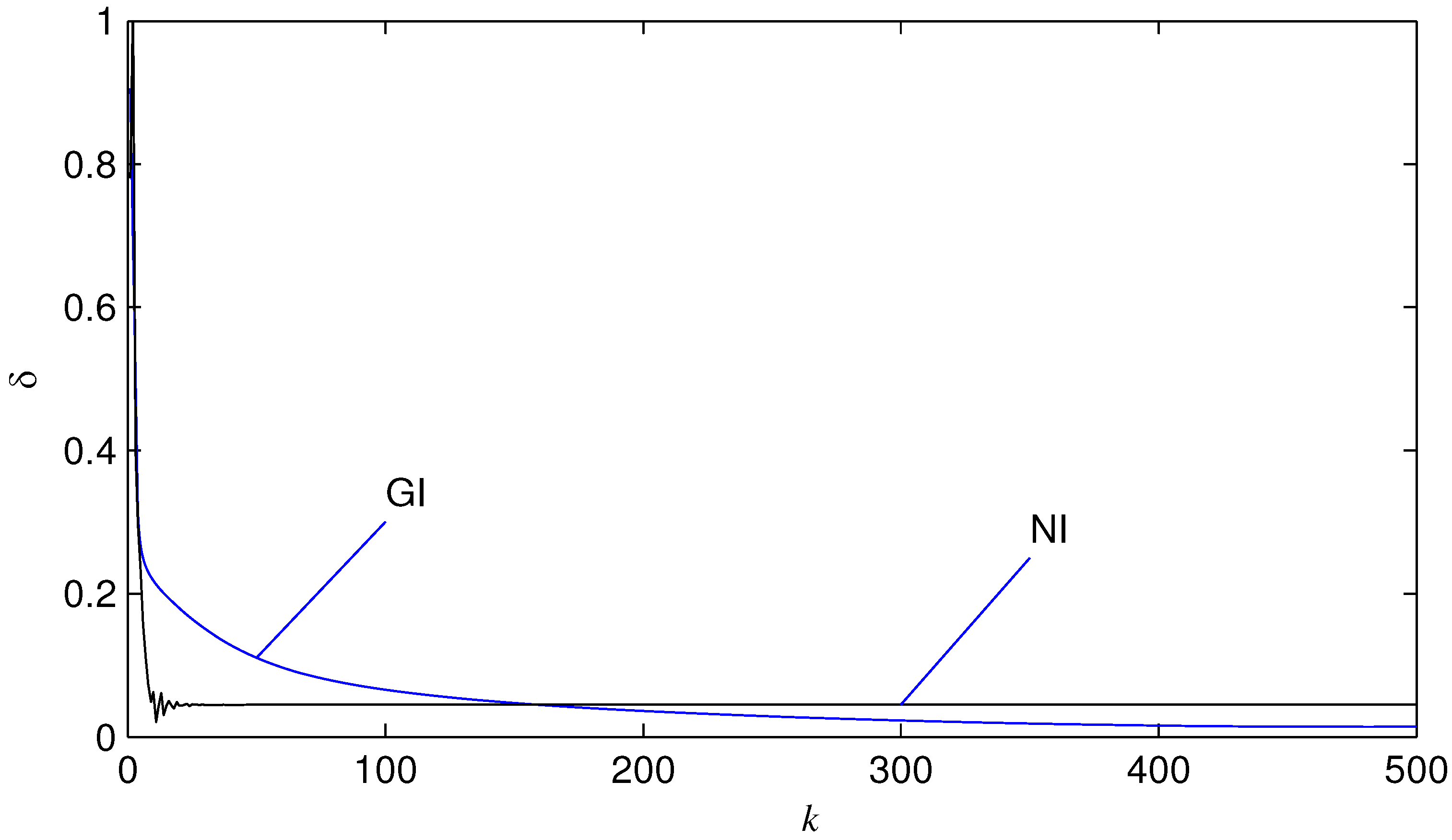
  • The NI algorithm has a faster convergence rate than the GI algorithm, but the GI algorithm can generate more accurate parameter estimates than the NI algorithm: see the error curves in Figure 3.
Table 1. The parameter estimates (ai, bi, γi, di) and their errors (σ2 = 0.402).
ka1a2b1b2γ2γ3d1δ(%)
100.022150.407931.004460.111680.493140.273430.1540020.88476
500.141130.439500.973190.235920.534380.277360.179338.15348
1000.193820.440380.975560.295950.528700.268520.211573.04925
2000.214020.441220.990650.324700.509130.248970.235492.97170
3000.216920.441270.996010.330170.502790.243040.241453.59966
4000.217570.441270.997440.331490.501140.241520.243143.79156
5000.217730.441270.997800.331820.500710.241120.243643.84560
True values0.200000.440000.990000.300000.500000.250000.21000
Table 2. The parameter estimates (ai, bi, γi, di) and their errors (σ2 = 0.202).
ka1a2b1b2γ2γ3d1δ (%)
100.021150.408021.020950.107350.474320.256700.1271521.79777
500.130190.439640.980930.221180.520430.270020.1206711.04226
1000.183730.439850.977220.280550.523390.268970.136876.58059
2000.205640.440440.988540.309490.508920.253550.165583.61544
3000.208650.440510.993260.314700.503280.248150.185292.28582
4000.209270.440540.994540.315910.501700.246700.199701.57463
5000.209430.440570.994890.316220.501220.246280.210441.39000
True values0.200000.440000.990000.300000.500000.250000.21000

5. Conclusions

In this paper we have derived the gradient-based iterative identification algorithm for Wiener nonlinear OEMA systems. The proposed algorithm can simultaneously estimate the parameters of the linear and nonlinear parts of Wiener nonlinear OEMA systems. The simulation results showed the parameters of Wiener nonlinear OEMA systems can be estimate effectively by the proposed algorithm. The method in the paper can be applied to study identification problems for other linear or nonlinear systems.

Acknowledgments

This work was supported by the Natural Science Foundation of the Jiangsu Higher Education Institutions of China (No. 15KJB120001), the Foundation of the Changshu Institute of Technology, China (Nos. KYZ2015006Z, KYZ2015007Z), Talent Peak of Six Industries of Jiangsu Province (2014-NY-021), and Qing Lan Project of Jiangsu Province.

Author Contributions

Lincheng Zhou prepared the manuscript and the simulation. Huigang Xu and Peiyi Zhu assisted in the revising work and the simulation. Xiangli Li was in charge of the overall research and critical revision of the paper.

Conflicts of Interest

The authors declare no conflict of interest.

References

  1. Ding, F.; Liu, X.P.; Liu, G. Identification methods for Hammerstein nonlinear systems. Digit. Signal Proc. 2011, 21, 215–238. [Google Scholar] [CrossRef]
  2. Li, J.H. Parameter estimation for Hammerstein CARARMA systems based on the Newton iteration. Appl. Math. Lett. 2013, 26, 91–96. [Google Scholar] [CrossRef]
  3. Chen, J.; Wang, X.P.; Ding, R.F. Gradient based estimation algorithm for Hammerstein systems with saturation and dead-zone nonlinearities. Appl. Math. Model. 2012, 36, 238–243. [Google Scholar] [CrossRef]
  4. Yu, L.; Zhang, J.B.; Liao, Y.; Ding, J. Parameter estimation error bounds for Hammerstein finite impulsive response models. Appl. Math. Comput. 2008, 202, 472–480. [Google Scholar] [CrossRef]
  5. Li, X.L.; Ding, R.F.; Zhou, L.C. Least-squares-based iterative identification algorithm for Hammerstein nonlinear systems with non-uniform sampling. Int. J. Comput. Math. 2013, 90, 1524–1534. [Google Scholar] [CrossRef]
  6. Wang, Y.Y.; Wang, X.D.; Wang, D.Q. Identification of Dual-Rate Sampled Hammerstein Systems with a Piecewise-Linear Nonlinearity Using the Key Variable Separation Technique. Algorithms 2015, 8, 366–379. [Google Scholar] [CrossRef]
  7. Vörös, J. Parameter identification of Wiener systems with multisegment piecewise-linear nonlinearities. Syst. Control Lett. 2007, 56, 99–105. [Google Scholar] [CrossRef]
  8. Zhou, L.C.; Li, X.L.; Pan, F. Gradient based iterative parameter identification for Wiener nonlinear systems. Appl. Math. Model. 2013, 37, 8203–8209. [Google Scholar] [CrossRef]
  9. Zhou, L.C.; Li, X.L.; Pan, F. Gradient-based iterative identification for Wiener nonlinear systems with non-uniform sampling. Nonlinear Dyn. 2014, 76, 627–634. [Google Scholar] [CrossRef]
  10. Chen, J. Gradient based iterative algorithm for wiener systems with piece-wise nonlinearities using analytic parameterization methods. Comput. Appl. Chem. 2011, 28, 855–857. [Google Scholar]
  11. Zhou, L.C.; Li, X.L.; Pan, F. Gradient-based iterative identification for MISO Wiener nonlinear systems: Application to a glutamate fermentation process. Appl. Math. Model. 2013, 26, 886–892. [Google Scholar] [CrossRef]
  12. Pelckmans, K. MINLIP for the identification of monotone Wiener systems. Automatica 2011, 47, 2298–2305. [Google Scholar] [CrossRef]
  13. Wang, D.Q.; Ding, F. Least squares based and gradient based iterative identification for Wiener nonlinear systems. Signal Process. 2011, 91, 1182–1189. [Google Scholar] [CrossRef]
  14. Hagenblad, A.; Ljung, L.; Wills, A. Maximum likelihood identification of Wiener models. Automatica 2008, 44, 2697–2705. [Google Scholar] [CrossRef]
  15. Liu, Y.J.; Ding, F.; Shi, Y. Least squares estimation for a class of non–uniformly sampled systems based on the hierarchical identification principle. Circuits Syst. Signal Process. 2012, 31, 1985–2000. [Google Scholar] [CrossRef]
  16. Liu, Y.J.; Wang, D.Q.; Ding, F. Least squares based iterative algorithms for identifying Box-Jenkins models with finite measurement data. Digit. Signal Process. 2010, 20, 1458–1467. [Google Scholar] [CrossRef]
  17. Chen, H.; Lv, X.; Qiao, Y. Application of gradient descent method to the sedimentary grain-size distribution fitting. J. Comput. Appl. Math. 2009, 233, 1128–1138. [Google Scholar] [CrossRef]
  18. Chen, J.; Ding, F. Modified stochastic gradient algorithms with fast convergence rates. J. Vib. Control 2011, 17, 1281–1286. [Google Scholar] [CrossRef]
  19. Jiang, H.; Wilford, P. A stochastic conjugate gradient method for the approximation of functions. J. Comput. Appl. Math. 2012, 236, 2529–2544. [Google Scholar] [CrossRef]
  20. Calo, V.M.; Collier, N.; Gehre, M.; Jin, B.; Radwan, H.; Santillana, M. Gradient-based estimation of Manning’s friction coefficient from noisy data. J. Comput. Appl. Math. 2013, 238, 1–13. [Google Scholar] [CrossRef]
  21. Ding, J.; Shi, Y.; Wang, F.; Ding, H. A modified stochastic gradient based parameter estimation algorithm for dual-rate sampled-data systems. Digit. Signal Process. 2010, 20, 1238–1249. [Google Scholar] [CrossRef]
  22. Liu, Y.J.; Yu, L.; Ding, F. Multi-innovation extended stochastic gradient algorithm and its performance analysis. Circuits Syst. Signal Process. 2010, 29, 649–667. [Google Scholar] [CrossRef]
  23. Ding, F.; Liu, X.P.; Liu, G. Gradient based and least-squares based iterative identification methods for OE and OEMA systems. Digit. Signal Process. 2010, 20, 664–677. [Google Scholar] [CrossRef]
  24. Xie, L.; Yang, H.Z. Gradient based iterative identification for non-uniform sampling output error systems. J. Vib. Control 2011, 17, 471–478. [Google Scholar] [CrossRef]
  25. Xiong, W.L.; Ma, J.X.; Ding, R.F. An iterative numerical algorithm for modeling a class of Wiener nonlinear systems. Appl. Math. Lett. 2013, 26, 487–493. [Google Scholar] [CrossRef]
  26. Wang, D.Q.; Yang, G.W.; Ding, R.F. Gradient-based iterative parameter estimation for Box-Jenkins systems. Comput. Math. Appl. 2010, 60, 1200–1208. [Google Scholar] [CrossRef]
  27. Li, J.H.; Ding, R.F.; Yang, Y. Iterative parameter identification methods for nonlinear functions. Appl. Math. Model. 2012, 36, 2739–2750. [Google Scholar] [CrossRef]
  28. Zhang, Z.N.; Ding, F.; Liu, X.G. Hierarchical gradient based iterative parameter estimation algorithm for multivariable output error moving average systems. Comput. Math. Appl. 2011, 61, 672–682. [Google Scholar] [CrossRef]
  29. Wang, D.Q.; Chu, Y.Y.; Ding, F. Auxiliary model-based RELS and MI-ELS algorithms for Hammerstein OEMA systems. Comput. Math. Appl. 2010, 59, 3092–3098. [Google Scholar] [CrossRef]
  30. Liu, M.M.; Xiao, Y.S.; Ding, R.F. Iterative identification algorithm for Wiener nonlinear systems using the Newton method. Appl. Math. Model. 2013, 37, 6584–6591. [Google Scholar] [CrossRef]

