A Comparative Study of Modern Heuristics on the School Timetabling Problem

Abstract

In this contribution a comparative study of modern heuristics on the school timetabling problem is presented. More precisely, we investigate the application of two population-based algorithms, namely a Particle Swarm Optimization (PSO) and an Artificial Fish Swarm (AFS), on the high school timetabling problem. In order to demonstrate their efficiency and performance, experiments with real-world input data have been performed. Both algorithms proposed manage to create feasible and efficient high school timetables, thus fulfilling adequately the timetabling needs of the respective high schools. Computational results demonstrate that both algorithms manage to reach efficient solutions, most of the times better than existing approaches applied to the same school timetabling input instances using the same evaluation criteria.

1. Introduction

The problem faced in this contribution belongs to the wide family of educational timetabling problems which are NP-complete in their general form [1,2]. The main categories of educational timetabling problems are examination timetabling, university course timetabling, and high school timetabling [3]. In the current work we focus on the high school timetabling problem, which involves the weekly scheduling for all lecturers of a high school.

The school timetabling problem requires the assignment of lectures (events) to timeslots in such a way that no teacher/class (resources) is involved in more than one lecture simultaneously, while many other significant constraints are satisfied. These constraints include both hard and soft constraints. Hard constraints must be satisfied by all means, while soft constraints represent preferences and are used to evaluate the solution’s quality [4]. The goal is to find a feasible solution, satisfying all hard constraints, which is as qualitative as possible; that is, satisfying the maximum number of soft constraints. In the respective literature many variants of the high school timetabling problem have been presented, which mainly differ due to the educational system of each country [5,6,7]. In recent years many papers have been published describing specific techniques applied to the high school timetabling problem [8,9,10,11,12,13,14,15].

In current work, we investigate the application of two heuristic algorithms on the Greek school timetabling problem, namely Particle Swarm Optimization (PSO) [16] and Artificial Fish Swarm (AFS) [17]. The algorithms are applied to real-world input data coming from different Greek high schools. Simulation results demonstrate that both algorithms proposed manage to create feasible and efficient high school timetables, thus adequately fulfilling the timetabling needs of the respective high schools. The specific input instances used for their performance evaluation and comparison is the well-established Beligiannis benchmark [7]. This school timetabling data set has been already used as a benchmark by many researchers in the respective literature [6,7,18,19].

The PSO algorithm presented in current contribution is based on the PSO algorithm introduced in [20]. However, the proposed algorithm has significant differences compared to that algorithm, which are the following (see Section 3.1 for more details):

• The population size of the PSO based algorithm used in current work equals 15, while in [20] equals to 50.
• In the proposed PSO algorithm procedure SwapWithProbability() is applied to two randomly selected timeslots, while in [20] one of the two timeslots selected should have a hard clash (if such a timeslot exists).
• In [20] procedure SwapWithProbability() accepts swaps causing a hard clash with probability 2.2%, while in current algorithm this probability is set to 50%.
• In the proposed PSO algorithm procedure SwapWithProbability() accepts swaps which cause a raise in the individual’s fitness with probability equal to 0.5% while in [20] this probability is set to 2.2%.
• In [20] the probability of exiting the While Loop Structure which purpose is to produce a new particle with at least equal fitness value to the fitness value of the global best of the current generation, for each given particle, is set to 1.1%, while in current algorithm this probability is set to 1.08%.

These differences enable the proposed PSO algorithm to perform significantly better compared to the PSO algorithm presented in [20] as demonstrated by experimental results in Section 4.

The AFS algorithm presented in current contribution is a novel approach since, although there are plenty of population based algorithms applied to timetabling problems in the literature, there is no specific AFS based approach, to the best of our knowledge, applied to the high school timetabling problem. The structure of the proposed AFS approach is given in detail in Section 3.2.

Both algorithms presented in the current contribution use the same formalism for modeling the timetabling problem, try to minimize the same fitness function, and use the same performance criteria in order to evaluate the quality of each resulted timetable. Thus, a straightforward comparison of their experimental results is fair. Additionally, since there are other approaches in the respective literature using the same fitness function and evaluation criteria [21], a comparison of the proposed heuristic approaches with other approaches can be also performed on a fair basis.

All timetables created by the proposed algorithms are compared on the basis of three criteria, which are well-established school timetabling performance criteria in the respective literature. The first criterion, which investigates how evenly each teacher’s hours are distributed among the days she/he is available at school, is the teachers’ teaching hours’ distribution. The second criterion, which presents how uniformly distributed are the hours of the same lesson for each class among its teaching days, is the lessons’ hours’ distribution. Finally, the third criterion, which checks whether there are idle hours between teaching hours of each teacher, is the teachers’ gaps.

Numerical results demonstrate that both proposed algorithms achieve very satisfactory results and justify that modern heuristics constitute a very useful family of algorithms to cope effectively with this kind of problems. Moreover, one major advantage of the proposed algorithms lies in their inherent adaptive behavior. More specifically, both algorithms, by assigning weights that can be defined by the user to each specific constraint that should be satisfied, are able to fulfill adequately different timetabling needs of each respective school.

This paper is organized as follows. In Section 2 we present the mathematical model of the school timetabling problem faced. Section 3 describes the structure and operation of the proposed algorithms. Section 4 assesses and compares the performance of the proposed algorithms to each other and to that of existing approaches. Finally, Section 5 summarizes the conclusions and presents future work.

2. Problem Definition

The problem faced in this contribution is the weekly high school timetabling. This problem is affected by many parameters and has to satisfy a large number of hard and soft constraints [21]. Hard constraints are the ones that have to be fulfilled in order a timetable to be feasible, while soft constraints are the ones that affect the quality of a timetable. In Section 2.1, we list all hard and soft constraints considered in current contribution, while in Section 2.2 we present the mathematical model of the problem at hand.

2.1. Constraints

The hard constraints considered in current contribution are the following:

• Teachers’ clash: each teacher can teach to only one class at a given time period.
• Classes’ clash: each class can be taught only one lesson at a given time period.
• Teachers-classes-lessons assignment: each teacher can teach a limited number of hours and lessons to each class, which is predefined by input data.
• Teachers’ availability: each teacher can teach only in periods he/she is available, which is predefined by input data.
• Classes’ idle timeslots: must be only at the last hour of a day.
• Co-teaching restrictions: two or more teachers who teach the same lesson to the same class must be assigned to it at the same time period. For example, one class can be firstly joined with another class and then divided into two sub-classes, one for “English language for beginners” and one for “English language for intermediates” [22].
• Sub-classes restrictions: two or more teachers who teach different lessons to the same class at the same time period must be simultaneously assigned to it. For example, one class can be divided into two sub-classes, one for “Gymnastics” and one for “Economics” [22].

For a more detailed description of how both presented algorithms deal with co-teaching and sub-classes cases the interested reader can refer to [20].

The soft constraints considered in current contribution are the following:

• Teachers’ teaching hours’ distribution: checks how evenly each teacher’s hours are distributed among the days she/he is available at school.
• Lessons’ hours’ distribution: checks how uniformly distributed are the hours of the same lesson for each class among its teaching days.
• Teachers’ gaps: checks whether there are idle hours between teaching hours of each teacher.

2.2. Mathematical Model

The necessary data sets needed for the problem’s model definition are the following:

• $T=\left\{1,\dots ,TeachersNo\right\}$; the set of teachers
• $C=\left\{1,\dots ,ClassesNo\right\}$; the set of classes
• $D=\left\{1,\dots ,DaysNo\right\}$; the set of teaching days in a week
• $L=\left\{1,\dots ,LessonsNo\right\}$; the set of lessons
• $H=\left\{1,\dots ,HoursNo\right\}$; the set of teaching hours in a day
• $H_t^{not available}$; the set of time periods teacher t is not available at school
• $H_{last}$; the set of the last hours of all days
• $U$; a set of tuples $\left(m,n\right)$ for $m,n\in P:n\ge m+1$
• $E$; a set of meetings (events) such that to each meeting $e\in E$ a class-teacher pair and a given number of lessons that must be scheduled is preassigned [23]
• $E_t$; a set of meetings assigned to teacher t

The necessary variables and functions needed for the problem’s model definition are the following:

• $x_{tcdh}=\{\begin{array}{c}1,\text{ if teacher }t\text{ teaches class }c\text{ at day }d\text{ at hour }h\\ 0,\text{ if teacher }t\text{ does not teach class }c\text{ at day }d\text{ at hour }h\end{array}$
• $y_{lcdh}=\{\begin{array}{c}1,\text{ if lesson }l\text{ is taught at class }c\text{ at day }d\text{ at hour }h\\ 0,\text{ if lesson }l\text{ is not taught at class }c\text{ at day }d\text{ at hour }h\end{array}$
• $\chi \left(\alpha \right)=\{\begin{array}{c}1,\text{ if }\alpha \text{ is true}\\ 0,\text{ if }\alpha \text{ is false}\end{array}$
• $UpperBoun{d}_{td}$ is the maximum number of teaching hours that can be assigned to teacher t at day d so as his/her teaching hours are uniformly distributed
• $LowerBoun{d}_{td}$ is the minimum number of teaching hours that can be assigned to teacher t at day d so as his/her teaching hours are uniformly distributed
• $Subject{s}_{tc}$ is the number of different subjects that teacher t teaches to class c
• $Teacher\_Total\_Hour{s}_t$ is the total number of teaching hours that teacher t can teach in a week
• $Class\_Total\_Hour{s}_c$is the total number of teaching hours that class c can be taught in a week
• $z_{tdnm}$ is the idle times of teacher t between time slots m and n on day d [23]
• $v_{edp}=\{\begin{array}{ll}1,& \text{if the event }e\text{ is scheduled to timeslot }\left(d,p\right)\\ 0,& \text{otherwise}\end{array}$

Except for that, the following soft constraint costs are defined:

• $teacher{s}^{\prime }teaching hours\text{'} distribution cost=sc{w}_1\times {\displaystyle \sum }_{t=1}^T{\displaystyle \sum }_{d=1}^D{D}_{td},$ where

  $$D_{td}=\{\begin{array}{l}1,if\left({\displaystyle \sum _{c=1}^c{x}_{tcdh}\ge UpperBoun{d}_{td}+1}\right)\vee \left({\displaystyle \sum _{c=1}^c{x}_{tcdh}\le Loweroun{d}_{td}-1}\right),\forall t\in T,d\in D,h\in H\\ \hspace{0.17em}\hspace{0.17em}\hspace{0.17em}\hspace{0.17em}\hspace{0.17em}\hspace{0.17em}\hspace{0.17em}\hspace{0.17em}\hspace{0.17em}\hspace{0.17em}0,\text{ otherwise}\end{array}$$

  and $sc{w}_1$ is the respective soft constraint weight as described in [20].
• $lesson{s}^{\prime }hours\text{'} distribution cost=sc{w}_2\times {\displaystyle \sum }_{t=1}^T{G}_{tcd},$ where $G_{tcd}=\{\begin{array}{ll}1,& if {\displaystyle \sum }_{h=1}^H{x}_{tcdh}\ge Subject{s}_{tc}, \forall t\in T , c\in C, d\in D\\ 0,& \text{otherwise}\end{array}$ and $sc{w}_2$ is the respective soft constraint weight as described in [20]. If ${\displaystyle \sum }_{\text{h}=1}^{\text{H}}{\text{x}}_{\text{tcdh}}\ge {\text{ Subjects}}_{\text{tc}}$, this means that teacher t teaches, at least one subject, at class c at day d more than one hour (twice or more).
• $teacher{s}^{\prime }gaps cost=sc{w}_3\times {\displaystyle \sum }_{d=1}^D{\displaystyle \sum }_{\left(m,n\right)\in U}{z}_{tdmn},$ where $z_{tdmn}\ge 0, \forall t\in T, d\in D, \left(m,n\right)\in U$ and $z_{tdmn}\ge \left(n-m-1\right)\times \left(-1+{\displaystyle \sum }_{e\in E_t}\left(v_{edm}+v_{edn}-{\displaystyle \sum }_{m<p<n}{v}_{edp}\right)\right), \forall t\in T, d\in D, \left(m,n\right)\in U$.
  The latter inequality defines that, if variables are activated and there are no teaching periods between them, the value of $z_{tdmn}$ equals $\left(n-m-1\right)$ which is the number of idle times between m and n. This formulation of teachers’ gaps cost was firstly presented in [23]. Accordingly, $sc{w}_3$ is the respective soft constraint weight as described in [20].

Thus, the mathematical model of the problem can be expressed as follows:

$$min\left(teacher{s}^{\prime }teaching hours\text{'} distribution cost+lesson{s}^{\prime }hour{s}^{\prime }distribution cost+teacher{s}^{\prime }gaps cost\right) ,\forall t\in T, c\in C, l\in L, d\in D, h\in H, e\in E$$

under the following constraints:

• ${{\displaystyle \sum }}_{t=1}^T\chi \left(\left(x_{t{c}_{i}dh}=1\right)\wedge \left(x_{t{c}_{j}dh}=1\right)\right)\le 0, \forall c_i,c_j\in C \left(i\ne j\right), d\in D, h\in H$; (Teachers’ clash)
• ${{\displaystyle \sum }}_{c=1}^C\chi \left(\left(x_{l_{i}cdh}=1\right)\wedge \left(x_{l_{j}cdh}=1\right)\right)\le 0, \forall l_i,l_j\in L \left(i\ne j\right), d\in D, h\in H$; (Classes’ clash)
• ${{\displaystyle \sum }}_{c=1}^C{{\displaystyle \sum }}_{d=1}^D{{\displaystyle \sum }}_{h=1}^H{x}_{tcdh}=Teacher\_Total\_Hour{s}_t, \forall t\in T$; (Teachers’ teaching hours)
• ${{\displaystyle \sum }}_{t=1}^T{{\displaystyle \sum }}_{d=1}^D{{\displaystyle \sum }}_{h=1}^H{x}_{tcdh}=Class\_Total\_Hour{s}_c, \forall c\in C$; (Classes’ teaching hours)
• ${{\displaystyle \sum }}_{t=1}^T\chi \left(\left(x_{tcdh}=1\right)\wedge h\in H_t^{not available}\right)\le 0, \forall c\in C , d\in D, h\in H$; (Teachers’ availability)
• ${{\displaystyle \sum }}_{c=1}^C\chi \left(\left(y_{lcdh}=0\right)\wedge h H_{last}\right)\le 0, \forall l\in L , d\in D, h\in H$; (Classes’ idle time slots)
• ${{\displaystyle \sum }}_{c=1}^C\chi \left(\left(x_{t_{i}cdh}=1\right)\wedge \left(x_{t_{j}cdh}=1\right)teachers t_i and t_{j}are not involved in co-teaching\right)\le 0$, $\forall t_i,t_j\in T \left(i\ne j\right), d\in D, h\in H$; (co-teaching/sub-classes)

3. The Proposed Algorithms

3.1. Description of the Proposed PSO Algorithm

The population of the proposed PSO algorithm consists of 15 particles, each one comprising a two-dimensional array. Although the population size is different from the one used in [20], the particle encoding is the same. The number of rows of each particle equals the number of different classes of each school, while the number of columns is 35, since the timeslots of a weekly Greek school timetable are 35 at the most [20]. Each particle’s cell contains a number ranging from 1 to the number of different teachers of each school or a “−1” value. For example, if cell [i,j] equals “4”, that means that the 4th teacher teaches one of his/her lessons at the i-th class at the j-th timeslot. If cell [i,j] equals “−1”, that means that the i-th class has the j-th timeslot empty. The interested reader can find more details about the particle encoding used in [20].

In Algorithm 1, the pseudo code of the proposed PSO based algorithm is presented. The algorithm is a hybrid one consisting of two basic components:

• the main algorithm, which has four basic differences compared to the algorithm presented in [20].
• a local search procedure, which is the same as the one used in [20] and aims improving the quality of the resulted timetable after the execution of the main algorithm.

In this contribution we limit our description on the main algorithm, since all differences between the proposed PSO algorithm and the one presented in [20] lie there. The interested reader can find more details about the local search procedure in [20]. The differences of the proposed PSO algorithm compared to the algorithm presented in [20] are the following:

• Line 3: The number of particles P (i.e., the population size) is set to 15, while in [20] equals 50.
• Lines 22–23: Procedure SwapWithProbability() is applied to two randomly selected timeslots, while in [20] one of the two timeslots selected should have a hard clash (if such a timeslot exists).
• Line 22: Procedure SwapWithProbability() accepts swaps causing a hard clash with probability equal to 50%, while in [20] this probability equals 2.2%.
• Line 22: Procedure SwapWithProbability() accepts swaps which cause a raise in the individual’s fitness with probability equal to 0.5%, while in [20] this probability equals 2.2%.
• Lines 29–34: The probability of exiting the While Loop Structure is set to 1.08%, while in [20] equals 1.1%.

Algorithm 1: The pseudo code of the main PSO algorithm.

In what follows, P is the number of particles (i.e., the population size), particle(p) is the p-th particle of the population, Personal_best(p) is the personal best achieved by particle p till current generation and Global_best is the globally best particle among all particles till current generation, i.e. the particle with smallest fitness. In addition, F() stands for the fitness function, F stands for the fitness function value, while auxiliary_particle is a structure identical to any particle’s structure that serves for temporal storage of a particle.

1. Start of hybrid PSO algorithm

2.    Start of main algorithm

3.    Read input Data; // i.e. teachers, classes, hours, co teachings etc.

4.    Initialize P particles with random structure;

5.    For each particle(p) {

6.       Personal_best(p) ← particle(p);

7.       F(Personal_best(p)) ← F(particle(p));

8.    } // end For

9.    Global_best ← the particle with smallest fitness;

10.    F(Global_best) ← the smallest fitness among all particles;

11.    While generation < numOfGenerations {  // numOfGenerations is set to 10,000

12.             For each particle(p) {

13.                 F(particle(p)) ← compute fitness of particle(p);

14.                 If (F(particle(p)) <= F(Personal_best(p)) then {

15.                       F(Personal_best(p)) ← F(particle(p));

16.                       Personal_best(p) ← particle(p);

17.                       If F(particle(p) <= F(Global_best) then {

18.                            F(Global_best) ← F(particle(p));

19.                            Global_best ← particle(p);

20.                       } // end If

21.                 } // end If

22.                 Select two different timeslots t1, t2 at random;

23.                 Execute procedure SwapWithProbability(particle(p), t1, t2);

24.                 Select a timeslot t at random;

25.                 Execute procedure InsertColumn(Personal_best(p), particle(p), t);

26.                 Select a timeslot t at random;

27.                 Execute procedure InsertColumn(Global_best, particle(p), t);

28.                 F_before_entering_While_Loop_Structure ← F(particle(p));

29.                 auxiliary_particle ← particle(p);

30.                 While F(particle(p)) > F(Global_best) { // this is the While Loop Structure

31.                       Every 10 loop-cycles break the while-loop with a fixed probability;

32.                      Select a timeslot t at random;

33.                       Execute procedure InsertColumn(Global_best, particle(p), t);

34.                       F(particle(p)) ← compute fitness of particle(p);

35.                 } // end While (While Loop Structure)

36.                 If F(particle(p)) > F_before_entering_While_Loop_Structure then {

37.                       particle(p) ← auxiliary_particle;

38.                       F(particle(p)) ← F_before_entering_While_Loop_Structure;

39.                 } // end If

40.       } // end For each particle(p)

41.    ++generation;

42.    } // end While termination criterion is not met

43.    End of main algorithm //Here is where the main algorithm ends and the refinement phase starts

44.    Execute Local Search Procedure

45.    output ← Global_best;

46. End of hybrid PSO algorithm

As seen in Algorithm 1, the main algorithm involves three major components, namely, procedure SwapWithProbability(), procedure InsertColumn() and a While Loop Structure. These three parts are described in short in the next paragraphs. The interested reader can find more details about these parts in [20].

The parameters of procedure SwapWithProbability() are the current particle (particle(p)) and two different timeslots t₁ and t₂. Procedure SwapWithProbability() investigates all swaps between the cells of timeslots (columns) t₁ and t₂ for all classes of particle(p). Swaps that cause no hard clash and result in a smaller or equal fitness value are always accepted and executed. Swaps that cause hard constraint violations are accepted with probability equal to 50%. Swaps that do not cause hard constraint violations but lead to larger (worse) fitness function values are accepted with probability equal to 0.5%. Note that the acceptance of invalid swaps permits the algorithm to escape from local optima in most cases.

Procedure InsertColumn() is used in order to substitute timeslots of current particle (particle(p)) with timeslots either from the personal best of current particle (Personal_best(p)) or the global best (Global best) found until that point. Procedure InsertColumn() takes as first parameter either Personal_best(p) or Global_best, as second parameter particle(p) and as third parameter a random selected timeslot t, which is the timeslot to be replaced in particle(p) either from Personal_best(p) or Global_best.

The While Loop Structure tries to discover, for each particle(p), a particle with the best or equal fitness value to the fitness value of Global_best, by applying procedure InsertColumn() between Global_best and particle(p). In order to avoid being trapped into an infinite loop, the algorithm can exit the While Loop Structure with a probability set to 1.08%, no matter what the achieved fitness value is, every time 10 more loops are executed.

3.2. Description of the Proposed AFS Algorithm

The population of the proposed AFS algorithm consists of 24 fish, each of which is a two-dimensional array. The fish encoding is the same as the one used by the proposed PSO algorithm and the algorithm presented in [20]. In Algorithm 2, the pseudo code of the proposed AFS based algorithm is presented. The algorithm is a hybrid one consisting of two basic components:

• the main algorithm, which will be analytically described in the following paragraphs.
• a local search procedure, which is the same as the one used by the proposed PSO algorithm and the algorithm presented in [20].

As seen in Algorithm 2, the main algorithm includes seven basic procedures, namely, procedure Prey(), procedure InnerPrey(), procedure SwarmNChace(), procedure CreateNeighborhood(), procedure CalculateLocalCentre(), procedure Leap(), and procedure Turbulence(). A detailed description of these procedures is given in the following paragraphs.

We define Distance d between two fish f1 and f2 as the number of cells of the timetable, in which the two fish differ. The distance of two fish takes values in the interval [0, number of classes × 35]. As the algorithm progresses, the fish tend to approach each other and the population loses the desired diversity that allows fish to seek in wider solutions area. To prevent this phenomenon, a shaker process of the space of solutions is used, called procedure Turbulence() (Algorithm 2, Line 10). This procedure is activated when the current maximum distance between all fish becomes less than MIN_DISTANCE_COEF × number of classes × 35, wherein MIN_DISTANCE_COEF is a user defined “proximity factor”, constant throughout the execution of the algorithm. During the execution of procedure Turbulence(), a random fish, a random row (class) in this fish and two random periods are selected. Then, utilizing procedure Swap() teachers assigned to classes during these periods are swapped. Procedure Swap() is repeated a specified number of times, which in all experiments conducted was equal to TURBULENCE_ITERATIONS × NUMBER_OF_FISH, wherein TURBULENE_ITERATIONS is user defined, constant throughout the execution of the algorithm. The parameters of procedure Swap(), as used in procedure Turbulence(), are four: a randomly selected fish, a randomly selected row in this fish and two randomly selected columns in this fish. It swaps the values of two cells in the same row of the timetable of fish f, i.e., teachers who are assigned to the two periods of the timetable of the class.

Procedure Leap() (Algorithm 2, Line 12) is activated when the improvement of the obtained best fitness (i.e., the fitness of minGlobalFish) during the last LEAP_NUMBER generations is less than MIN_IMR, where LEAP_NUMBER and MIN_IMR are user defined and constant. Parameter MIN_IMR is the threshold of desired fitness’ rate improvement in order to start the Leap() procedure (see also Table 1). Procedure Leap() is triggered repeatedly until the desired rate of improvement has been achieved or 10 executions without desired rate of improvement have been completed. In order to achieve the desired rate of improvement, procedure Leap() applies procedure Approach(), which forces current fish f to approach minGlobalFish. Procedure Approach() is repeated, inside the body of procedure Leap(), a specified number of times, which in all experiments conducted was equal to NUMBER_OF_FISH.

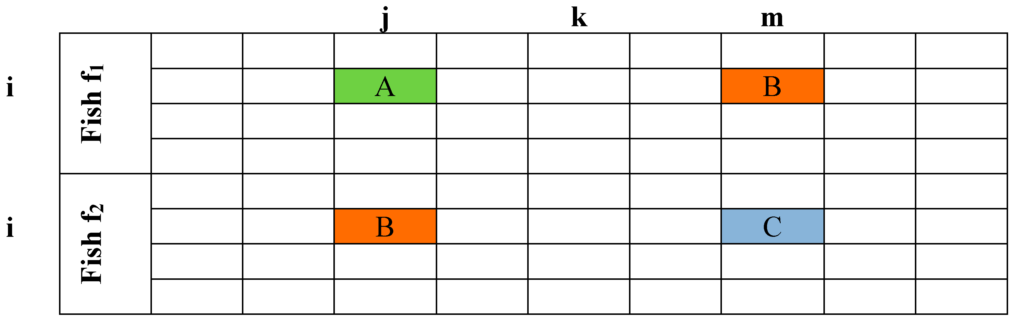
The Approach() procedure is one of the two procedures (the second one is RandomApproach() presented below) aimed to make fish f₁ approach fish f₂. To achieve this, it initially identifies the cells in which the teachers in the timetables of the two fish are different. 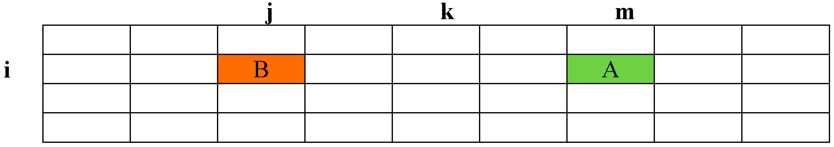So, if the values of fish f₁ and f₂ in cell (i, j) are different, say, “Professor A” and “Professor B”, then it is certain that there will be another cell (i, m), having “Professor B” as a value (this is assured by the initialization procedure) (Figure 1). Procedure Approach() is executed as follows: It randomly selects two cells of f₁ among cells in which timetables of f₁ and f₂ are different. Then, utilizing procedure Swap(), the algorithm switches the values of cells (i, j) and (i, m) of f₁ (Figure 2). In this way, the distance of the two fish is decreased by at least one unit (perhaps two if A = C). By choosing to make alternations per class (horizontal) we ensure that the number of hours that each teacher is assigned to each class is not violated (this has been ensured by the initialization procedure). The process ends when the percentage of the initial distance between the two fish becomes less than (1.0-STEP_RATIO), where STEP_RATIO is a user defined variable, constant throughout the execution of the algorithm.

Algorithm 2: The pseudo code of the main AFS algorithm.

In what follows, minGlobalFish is the fish with best fitness in population, personalBest is the current personal best structure of each fish, localBest is the fish with the best fitness in a neighborhood, localCentre is the centre of a fish neighborhood and leapNumber is the number of generations every which the algorithm checks whether an improvement over threshold MIN_IMPR in the fitness of minGlobalFish has occurred.

1. Start of hybrid AFS algorithm

2.    Start of main algorithm

3.    Read input Data; //i.e., teachers, classes, hours, co teachings etc.

4.    Create initial population of fish, each fish having random structure; //The size of initial population is set to NUMBER_OF_FISH=24

5.    minGlobalFish ← The fish with best fitness in population;

6.    Make every fish best position equal to current (i.e., initial) position;

7.    generation ← 0;

8.    While generation < NUM_OF_GENERATIONS { // NUM_OF_GENERATIONS is set to 10,000

9. If maximum distance between all fish is less than a minimum threshold then

// Threshold is equal to MIN_DISTANCE_COEF × number of classes × 35

10.                 Execute procedure Turbulence(); // perturb the population of fish

11. If the % improvement of minGlobalFish fitness for the last LEAP_NUMBER generations is not bigger than MIN_IMPR then

// MIN_IMPR is a threshold in the improvement of minGlobalFish

12.   Execute procedure Leap(); // make fish approach minGlobalFish

13.             For each fish f {

14.                 If fitness of fish f has been improved then

15.                       update fish f personalBest;

16.                 Execute procedure CreateNeighborhood(f); // recreate the neighborhood of fish f

17.             Execute procedure CalculateLocalCentre(f); // calculate the localCentre of the neighborhood of fish f and the localBest of fish f

18.             If the neighborhood of fish f is sparse then // if it contains less than SPARSE_COEF × NUMBER_OF_FISH members

19. Execute procedure Prey(f); // try to find for fish f, in the whole population, a structure having better fitness

20.                 Else

21.                If the neighborhood of fish f is dense then // if it contains more than DENSE_COEF × NUMBER_OF_FISH members

22. Execute procedure InnerPrey(f); // try to find for fish f, in its neighborhood, a structure having better fitness

23.                Else

24. Execute procedure SwarmNChase(f); // try to find for fish f a structure having better fitness in case its neighborhood is neither dense nor sparse

25.                 If fitness of fish f < = fitness of minGlobalFish then

26.                       minGlobalFish ← f;

27.             } // end For each fish f

28.    ++generation;

29.     } // end While generation < numOfGenerations

30.    End of main algorithm //Here is where the main algorithm ends and the refinement phase starts

31.    Execute Local Search Procedure

32.    output ← minGlobalFish;

33.  End of hybrid AFS algorithm

Figure 1. Two fish timetables which differ in cell (i, j).

Figure 1. Two fish timetables which differ in cell (i, j).

Figure 2. The fish f₁ after switching cells (i, j) and (i, m).

Figure 2. The fish f₁ after switching cells (i, j) and (i, m).

Procedure CreateNeighborhood() (Algorithm 2, Line 16) plays a major role in the operation of the algorithm. Its aim is to create in every generation, the current neighborhood for each fish. As the fish move, their mutual distances change and they are getting far or near to each other. Thus, neighborhoods of fish evolve dynamically during execution of the algorithm. This means that in every generation, the neighborhood of each fish is recalculated. We define that a fish f₁ is assumed to lie in the neighborhood of a fish f, if its distance from f is less than minDist + (maxDist – minDist) × VISUAL_SCOPE_COEF, where minDist and maxDist are respectively the minimum and maximum distance among all fish of current population and VISUAL_SCOPE_COEF is a user defined parameter, constant throughout the execution of the algorithm. As stated before, the distance d between two fish f1 and f2 is the number of cells of the timetable, in which the two fish differ. Procedure CreateNeighborhood() sets the fish in the neighborhood of f in increasing fitness order. So, the first fish in the neighborhood of f, is the one with the best fitness among all its neighbors. A neighborhood is considered “sparse” (Algorithm 2, Line 18), when containing less than SPARSE_COEF × NUMBER_OF_FISH members, where NUMBER_OF_FISH is the population size and SPARSE_COEF is a user defined parameter, constant throughout the execution of the algorithm. A neighborhood is considered “dense” (Algorithm 2, Line 21), when containing more than DENSE_COEF × NUMBER_OF_FISH members, where DENSE_COEF is a user defined parameter, constant throughout the execution of the algorithm.

One of the key behaviors simulated in AFS algorithms is the tendency of fish to gather in flocks to maximize food-finding and survival chances [17]. The concentration of fish in flocks (swarming) is simulated by moving the fish to a “notional” fish located in the “center” of their neighborhood (localCentre fish). This “notional” fish, is created by procedure CalculateLocalCentre() (Algorithm 2, Line 17). At first, the localCentre fish is set equal to the first fish in the neighborhood of f, which is the fish with the best fitness among all fish in the neighborhood, since procedure CreateNeighborhood() sets the fish in the neighborhood of f in increasing fitness order (see above). Then, for an arbitrary number of times (without, of course, exceeding the size of the neighborhood), the localCentre approaches the i-th fish of the neighborhood, utilizing procedure Approach(), with a diminishing step given by the expression $\frac{1}{i+1}$. For example, the localCentre approaches the second fish of the neighborhood with step equal to $\frac{1}{3}$, the third fish of the neighborhood with step equal to $\frac{1}{4}$ and so on. As a result, the participation of the most robust fish of the neighborhood to the creation of the localCentre is greater than that of the less robust.

A fish f performs Prey() (Algorithm 2, Line 19) procedure when its neighborhood is not rich enough in fish, towards which it could make a move. A fish f1, different from f, is selected randomly from fish population and if it has better fitness than f then fish f moves towards f1 using procedure RandomApproach() and procedure Prey() is completed. If the fitness of f1 is not better than the fitness of f then f can also move towards f1 using procedure RandomApproach() with probability equal to $e^{-\frac{dc}{gen}}$ (dc is the difference in fitness between fish f₁ and fish f and gen is the current generation) and procedure Prey() is completed, too. This is repeated PREY_TRY_NUMBER times at most, where PREY_TRY_NUMBER is a user defined parameter, constant throughout the execution of the algorithm. In case none of the above situations take place, fish f moves towards its personalBest using procedure RandomApproach(). The pseudo code of procedure Prey() is presented in Algorithm 3.

Algorithm 3: The pseudo code of procedure Prey().

0. For try ← 1 to PREY_TRY_NUMBER {

1. accept ← random number between 0 and 1;

2. pick a random fish f1 among the population;

3. dc ← fitness of f1 – fitness of f;

4. If fitness of f1 <= fitness of f then {

5. Execute procedure RandomApproach(); // move randomly fish f towards fish f1;

6. return;

7. } // end If

8. If (fitness of f1 > fitness of f) and ($e^{-\frac{dc}{gen}}$ > = accept) then {

9. Execute procedure RandomApproach(); // move randomly fish f towards fish f1;

10. return;

11. } // end If

12. } // end For

13. Execute procedure RandomApproach(); // move randomly fish f towards its personalBest

14. return;

Procedure RandomApproach() works the same way as procedure Approach(), with the difference that it completes its operation if f₁ achieves better fitness than its initial one during the execution of the procedure. It chooses, just like in procedure Approach(), a random location at which both fish differ and then tests all the swaps (in same way as described in procedure Approach()). From all these swaps, procedure RandomApproach() finally chooses to carry out the one that leads to better fitness among all available swaps. The process ends either when a better fitness to f₁ is achieved or when—as in procedure Approach()—the percentage of the initial distance between the two fish becomes less than (1.0-STEP_RATIO).

A fish f performs InnerPrey() (Algorithm 2, Line 22) procedure when its neighborhood is quite rich in fish, towards which it could make a move. A fish f₁, different from f, is selected randomly from the neighbors of f and if it has better fitness than f then fish f moves towards f₁ using procedure RandomApproach() and procedure InnerPrey() is completed. If the fitness of f₁ is not better than the fitness of f then f can also move towards f₁ using procedure RandomApproach() with probability equal to $e^{-\frac{dc}{gen}}$ (dc is the difference in fitness between fish f₁ and fish f and gen is the current generation) and procedure InnerPrey() is completed, too. This is repeated PREY_TRY_NUMBER times at most. In case none of the above situations take place, procedure Prey() is executed. The pseudo code of procedure InnerPrey() is presented in Algorithm 4.

Algorithm 4: The pseudo code of procedure InnerPrey().

0. For try ← 1 to PREY_TRY_NUMBER {

1. accept ← random number between 0 and 1;

2. pick a random fish f1 among its neighbors;

3. dc ← fitness of f1 – fitness of f;

4. If fitness of f1 <= fitness of f then {

5. Execute procedure RandomApproach(); // move randomly fish f towards fish f1;

6. return;

7. } // end If

8. If (fitness of f1 > fitness of f) and ($e^{-\frac{dc}{gen}}$ > = accept) then {

9. Execute procedure RandomApproach(); // move randomly fish f towards fish f1;

10. return;

11. } end If

12. } end For

13. Execute procedure Prey(); // See Algorithm 3

14. return;

A fish f performs procedure SwarmNChase() (Algorithm 2, Line 24) when its neighborhood is neither “dense” nor “sparse” in fish. Fish f, using procedure RandomApproach(), moves separately and independently to the localCentre fish of its neighborhood (swarm behavior) and to the localBest fish of its neighborhood (chase behavior) [17,24]. The fish f finally takes the move which gives better fitness. If neither of the two moves lead to better fitness, the fish executes procedure InnerPrey(). The pseudo code of procedure SwarmNChase() is presented in Algorithm 5.

Algorithm 5: The pseudo code of procedure SwarmNChase().

0. tempFish1 ← f;

1. tempFish2 ← f;

2. move randomly fish tempFish1 towards the localBest of neighborhood of f;

3. move randomly fish tempFish2 towards the localCentre of neighborhood of f;

4. tempFish ← fish with the minimum fitness among tempFish1 and tempFish2;

5. If fitness of tempFish <= fitness of f then

6. f ← tempFish;

7. Else

8. InnerPrey(f); // See Algorithm 4

9. Return;

As seen in the previous paragraphs, the proposed AFS algorithm uses many user-defined parameters that affect the algorithm’s convergence and efficiency. In Table 1 all user defined parameters are summarized and explained. Moreover, their values used in all experiments are listed. Although the adjustment of user-defined parameter values remains an open issue, as there is no obvious way to tune them, after having conducted exhaustive experiments we decided to use the values presented in Table 1, since this combination of values resulted in the best performance of the proposed AFS algorithm.

Table 1. The user defined parameters used by the proposed AFS algorithm.

Parameter	Value	Comments
NUMBER_OF_GENERATIONS	10,000	The number of generations the algorithm is executed
NUMBER_OF_FISH	24	The size of the population of fish. We decided to use 24 fish since, after exhaustive experiments we came to the conclusion, that this is the minimum number of fish which guarantees that the AFS algorithm will always reach feasible solutions.
VISUAL_SCOPE_COEF	0.7	A fish f1 is located in the neighborhood of a fish f, if its distance from f is less than minDist + (maxDist – minDist) × VISUAL_SCOPE_COEF, where minDist and maxDist are respectively the minimum and maximum distance among all fish of current population
SPARSE_COEF	0.1	A neighborhood is considered “sparse”, when containing less than SPARSE_COEF × NUMBER_OF_FISH individuals
DENSE_COEF	0.8	A neighborhood is considered “dense”, when containing more than DENSE_COEF × NUMBER_OF_FISH individuals
STEP_RATIO	0.047	Fish approaching factor. Procedures Approach() and RandomApproach() are completed when the percentage of the initial distance between two fish becomes less than (1.0 - STEP_RATIO)
PREY_TRY_NUMBER	3	Number of iterations for procedures Prey() and InnerPrey()
MIN_DIST_COEF	0.01	The turbulence activating factor. Procedure Turbulence() is activated when the current maximum distance between all fish becomes less than MIN_DISTANCE_COEF × number of classes × 35
LEAP_NUMBER	100	Procedure Leap() is activated when the improvement of the obtained best fitness (i.e. the fitness of minGlobalFish) during the last LEAP_NUMBER generations is less than MIN_IMR
TURBULENCE_ITERATIONS	5	Number of repetitions of procedure Swap() inside procedure Turbulence() equals to TURBULENCE_ITERATIONS × NUMBER_OF_FISH
MIN_IMPR	0.01	Threshold of desired fitness’ rate improvement in order to start the Leap() procedure

Table 1. The user defined parameters used by the proposed AFS algorithm.

Parameter	Value	Comments
NUMBER_OF_GENERATIONS	10,000	The number of generations the algorithm is executed
NUMBER_OF_FISH	24	The size of the population of fish. We decided to use 24 fish since, after exhaustive experiments we came to the conclusion, that this is the minimum number of fish which guarantees that the AFS algorithm will always reach feasible solutions.
VISUAL_SCOPE_COEF	0.7	A fish f1 is located in the neighborhood of a fish f, if its distance from f is less than minDist + (maxDist – minDist) × VISUAL_SCOPE_COEF, where minDist and maxDist are respectively the minimum and maximum distance among all fish of current population
SPARSE_COEF	0.1	A neighborhood is considered “sparse”, when containing less than SPARSE_COEF × NUMBER_OF_FISH individuals
DENSE_COEF	0.8	A neighborhood is considered “dense”, when containing more than DENSE_COEF × NUMBER_OF_FISH individuals
STEP_RATIO	0.047	Fish approaching factor. Procedures Approach() and RandomApproach() are completed when the percentage of the initial distance between two fish becomes less than (1.0 - STEP_RATIO)
PREY_TRY_NUMBER	3	Number of iterations for procedures Prey() and InnerPrey()
MIN_DIST_COEF	0.01	The turbulence activating factor. Procedure Turbulence() is activated when the current maximum distance between all fish becomes less than MIN_DISTANCE_COEF × number of classes × 35
LEAP_NUMBER	100	Procedure Leap() is activated when the improvement of the obtained best fitness (i.e. the fitness of minGlobalFish) during the last LEAP_NUMBER generations is less than MIN_IMR
TURBULENCE_ITERATIONS	5	Number of repetitions of procedure Swap() inside procedure Turbulence() equals to TURBULENCE_ITERATIONS × NUMBER_OF_FISH
MIN_IMPR	0.01	Threshold of desired fitness’ rate improvement in order to start the Leap() procedure

4. Computational Results

The proposed algorithms were coded in C++ and run on i7–4770, 3.40 GHz and 16 GB of RAM, under the Windows 7 (64 bit) OS. All results presented in this section were accomplished using the same set of PSO parameters’ values for the PSO algorithm and the same set of AFS parameters’ values for the AFS algorithm. This was adopted in order to have a fair comparison of both algorithm’s efficiency and performance. Both algorithms use the same encoding described in Section 3.1 and Section 3.2. The population size was set to 15 for the PSO algorithm and to 24 for the AFS algorithm.

The fitness function used for both algorithms is the one presented in [20], incorporates all hard and soft constraints listed in Section 2 and has the following form:

• f = cases_of_teachers’_unavailability × HCW × BASE³
• + cases_of_classes’_empty_periods × HCW × (2 × BASE)^BASE
• + cases_of_parallel_teaching × HCW × BASE^k
• + cases_of_wrong_co-teaching × HCW × (2 × BASE)^BASE
• + cases_of_class_lessons’_dispersion × ICDW × HOURS × BASE^DAYS
• + cases_of_teachers’_empty_spaces × TEPW × HOURS × BASE^DAYS
• + cases_of_teacher_lessons’_dispersion × ITDW × absolute_error × BASE^DAYS

Moreover, all hard and soft constraints weights used in it have the exact same values as the ones used in [20] and are described as follows:

• Hard Constraints’ Weight (HCW). This weight is utilized by the algorithm in order to distinguish feasible and infeasible timetables. Its value is set to 10.
• Ideal Classes’ Dispersion Weight (ICDW). This weight is relevant to the classes’ lessons dispersion and its value is set to 0.95.
• Teachers’ Empty Periods Weight (TEPW). This weight relates to teachers’ idle hours during any working day and its value is set to 0.06.
• Ideal Teachers’ Dispersion Weight (ITDW). This weight is relevant to the teachers’ teaching hours’ dispersion and its value is set to 0.6.

Apart from the above weights, another major parameter that affects the behavior of the evaluation function is the exponential rise base (BASE). This is a real number (typically between 1 and 2) that is used as a base for the exponential rise of the sub-costs corresponding to violations of a certain constraints in a timetable. For all experiments conducted, its value was set to 1.3. In order to demonstrate the performance and efficiency of both computational intelligence algorithms, their experimental results are compared with the respective results of four different heuristics that have been applied to the school timetabling problem in the literature [19,20,25,26]. The approach presented in [19] is a simulated annealing (SA)-based algorithm with a newly-designed neighborhood structure. Its main innovation is that, in search for the best neighbor, the heuristic performs a sequence of swaps between pairs of timeslots, instead of swapping two assignments, as in the standard simulated annealing. The algorithm presented in [25] is an evolutionary one (EA). The algorithm uses linear ranking selection, two mutation operators, and an elitism schema, while, on the other hand, it does not use any crossover operator. The third algorithm presented in [20] comprises a hybrid particle swarm optimization (PSO)-based algorithm. It consists of a main PSO algorithm and a refining local search procedure which is applied in order to improve the best solution found by the main PSO algorithm. Finally, the fourth algorithm is a genetic algorithm selection perturbative hyper-heuristic (GASPHH) [26]. It comprises a two-phase approach, with the first phase focusing on hard constraints and the second phase on soft constraints. Both phases employ the same genetic algorithm selection perturbative hyper-heuristic, with the low-level heuristics differing for each phase.

Both algorithms presented in the current contribution, as well as the four algorithms mentioned in the previous paragraph, use the same formalism for modeling the timetabling problem and the same three performance criteria (teachers’ teaching hours’ distribution, lessons’ hours’ distribution and teachers’ gaps) in order to evaluate their performance. Thus, we can perform a straightforward and fair comparison of their experimental results. The input instances selected in order to compare the performance of these algorithms is the well-established Beligiannis data set [6,7], which has been used by all these algorithms in the respective contributions. In Table 2 the major characteristics of the input instances used in the experimental results are presented. The interested reader can find a thorough description of these instances in [19,20].

Table 2. Major characteristics of the Beligiannis school timetabling data set.

Instance	Number of Classes	Number of Teachers	Number of Teaching Hours	Number of Teachers Involvedin Co-Teaching	Number of Co-Teachings
1	11	34	385	9	36
2	11	35	385	17	67
3	6	19	210	0	0
4	7	19	245	6	31
5	6	18	184	0	0
7	13	35	455	17	70

Table 2. Major characteristics of the Beligiannis school timetabling data set.

Instance	Number of Classes	Number of Teachers	Number of Teaching Hours	Number of Teachers Involvedin Co-Teaching	Number of Co-Teachings
1	11	34	385	9	36
2	11	35	385	17	67
3	6	19	210	0	0
4	7	19	245	6	31
5	6	18	184	0	0
7	13	35	455	17	70

The proposed PSO algorithm as well as the proposed AFS algorithm is by nature stochastic. As a result, different computational results may be obtained in different runs. So, in order to demonstrate their efficiency, in Table 3 we present not only the best but also the worst and the average fitness achieved together with the respective standard deviation. The average execution time as well as the respective standard deviation is presented, too. In Table 4 the best performance of both proposed algorithms is compared with the best timetables created by the evolutionary algorithm (EA) presented in [25], the simulated annealing (SA) algorithm presented in [19], the hybrid PSO algorithm presented in [20] and the genetic algorithm selection perturbative hyper-heuristic (GASPHH) presented in [26].

The reason why we decided to present and compare the best timetables constructed by the proposed algorithms is that in [19,20,25,26] also the best timetables constructed are presented. Thus, in this way a fair comparison between all algorithms can be performed. Note that in order to compare two different timetables, we define one unit cost for any soft constraint violation among the three performance criteria (teachers’ teaching hours’ distribution, lessons’ hours’ distribution, and teachers’ gaps) [26]. All values presented in Table 3 and Table 4 are computed after executing 100 Monte Carlo runs. For both algorithms the average fitness achieved is very close to the best fitness. Additionally, the respective STD value is rather small. This demonstrates their efficiency and stability. Furthermore, the STD concerning the execution time of both algorithms is really small. This also demonstrates that both algorithms are very stable.

Table 3. Experimental results of the proposed stochastic algorithms.

Instance	Proposed PSO						Proposed AFS
	Fitness				Execution Time		Fitness				Execution Time
	Best	Worst	Average	STD	Average (min)	STD	Best	Worst	Average	STD	Average (min)	STD
1	11	21	16	2.5	36.6	3.4	16	31	22	3.8	120.8	2.4
2	18	28	22.1	2.5	47.8	0.8	21	34	28.6	3.7	147.2	1.1
3	5	9	7.4	0.8	3.9	0.4	7	13	10.4	1.7	28.5	0.9
4	5	13	8.8	2.2	13.2	0.3	9	23	14.5	3.2	59.4	2.6
5	0	0	0	0	3	0.1	0	5	2.4	1.5	24	0.1
7	23	49	35.8	6.8	57.9	0.4	32	88	56.1	14.1	168	3

Table 3. Experimental results of the proposed stochastic algorithms.

Instance	Proposed PSO						Proposed AFS
	Fitness				Execution Time		Fitness				Execution Time
	Best	Worst	Average	STD	Average (min)	STD	Best	Worst	Average	STD	Average (min)	STD
1	11	21	16	2.5	36.6	3.4	16	31	22	3.8	120.8	2.4
2	18	28	22.1	2.5	47.8	0.8	21	34	28.6	3.7	147.2	1.1
3	5	9	7.4	0.8	3.9	0.4	7	13	10.4	1.7	28.5	0.9
4	5	13	8.8	2.2	13.2	0.3	9	23	14.5	3.2	59.4	2.6
5	0	0	0	0	3	0.1	0	5	2.4	1.5	24	0.1
7	23	49	35.8	6.8	57.9	0.4	32	88	56.1	14.1	168	3

Table 4. Comparing the performance of both proposed algorithms with the algorithms presented in [19,20,25,26].

Instance	Proposed PSO	Proposed AFS	EA [25]	SA [19]	Hybrid PSO [20]	GASPHH [26]
1	11	16	70	29	15	60
2	18	21	76	37	17	66
3	5	7	20	8	7	17
4	5	9	41	28	8	43
5	0	0	10	3	0	15
7	23	32	109	40	32	83

Table 4. Comparing the performance of both proposed algorithms with the algorithms presented in [19,20,25,26].

Instance	Proposed PSO	Proposed AFS	EA [25]	SA [19]	Hybrid PSO [20]	GASPHH [26]
1	11	16	70	29	15	60
2	18	21	76	37	17	66
3	5	7	20	8	7	17
4	5	9	41	28	8	43
5	0	0	10	3	0	15
7	23	32	109	40	32	83

In Table 4 the best results, which are the best results found until today for the respective instances, are written in bold. The proposed PSO algorithm appears to have the best performance among all other algorithms achieving the best results ever found for 5/6 instances of the Beligiannis data set. The proposed AFS algorithm has also very satisfactory performance, since it surmounts the heuristic algorithms presented in [19,25,26]. At this point we have to call to mind that the proposed AFS algorithm uses many user-defined parameters that affect the algorithm’s convergence and efficiency. As a result, it is still an open issue to investigate thoroughly the best set of parameter values for the proposed AFS approach which will assist it to achieve even better results.

5. Conclusions

In this contribution a comparative study of modern heuristics on the school timetabling problem is presented. Two new heuristic population based algorithms, a particle swarm optimization (PSO) and an artificial fish swarm (AFS) one, are introduced and applied to the school timetabling problem. In order to demonstrate their efficiency and good performance both algorithms have been applied to the Beligiannis school timetabling data set and their results are compared with the results of four other heuristic algorithms published in the respective literature. Experimental results showed that the proposed PSO algorithm achieves the best results ever found for 5/6 instances of the Beligiannis data set. On the other hand, the proposed AFS algorithm, which comprises the first attempt to apply an AFS algorithm to the school timetabling problem in the literature, exhibits also very satisfactory results, since it overcomes three other heuristic approaches. This demonstrates that the AFS algorithm can be effectively applied to solve the school timetabling problem. The application of the proposed PSO algorithm to problems belonging to other timetabling or scheduling domains, as well as the investigation of the best set of parameter values for the proposed AFS approach, will be the main issues of our future work.

References

1. Cooper, T.B.; Kingston, J.H. The complexity of timetable construction problems. In Practice and Theory of Automated Timetabling; Springer Berlin Heidelberg: Berlin, Germany, 1996. [Google Scholar]
2. De Werra, D. The combinatorics of timetabling. Eur. J. Op. Res. 1997, 96, 504–513. [Google Scholar] [CrossRef]
3. Johnes, J. Operational research in education. Eur. J. Ope. Res. 2015, 243, 683–696. [Google Scholar] [CrossRef]
4. Tassopoulos, I.X.; Beligiannis, G.N. Using particle swarm optimization to solve effectively the school timetabling problem. Soft Comput. 2012, 16, 1229–1252. [Google Scholar] [CrossRef]
5. Pillay, N. Hyper-heuristics for educational timetabling. In Proceedings of the Ninth International Conference on the Practice and Theory of Automated Timetabling (PATAT 2012), Son, Norway, 28–31 August 2012; pp. 316–340.
6. Pillay, N. A survey of school timetabling research. Ann. Op. Res. 2014, 218, 261–293. [Google Scholar] [CrossRef]
7. Kristiansen, S.; Stidsen, T.R. A Comprehensive Study of Educational Timetabling—A Survey; Technical University of Denmark: Copenhagen, Denmark, 2013. [Google Scholar]
8. Raghavjee, R.; Pillay, N. A comparison of genetic algorithms and genetic programming in solving the school timetabling problem. In Proceedings of the Fourth World Congress on Nature and Biologically Inspired Computing (NaBIC 2012), Mexico City, Mexico, 5–9 November 2012; pp. 98–103.
9. Sørensen, M.; Kristiansen, S.; Stidsen, T.R. International timetabling competition 2011: An adaptive large neighborhood search algorithm. In Proceedings of the Ninth International Conference on the Practice and Theory of Automated Timetabling (PATAT 2012), Son, Norway, 28–31 August 2012; pp. 489–492.
10. Domrös, J.; Homberger, J. An evolutionary algorithm for high school timetabling. In Proceedings of the Ninth International Conference on the Practice and Theory of Automated Timetabling (PATAT 2012), Son, Norway, 28–31 August 2012; pp. 485–488.
11. Kalender, M.; Kheiri, A.; Özcan, E.; Burke, E.K. A greedy gradient-simulated annealing selection hyper-heuristic. Soft Comput. 2013, 17, 2279–2292. [Google Scholar] [CrossRef]
12. Kheiri, A.; Özcan, E.; Parkes, A.J. A stochastic local search algorithm with adaptive acceptance for high-school timetabling. Ann. Op. Res. 2014. [Google Scholar] [CrossRef] [Green Version]
13. Da Fonseca, G.H.G.; Santos, H.G.; Toffolo, T.A.M.; Brito, S.S.; Souza, M.J.F. GOAL solver: A hybrid local search based solver for high school timetabling. Ann. Op. Res. 2014, 1–21. [Google Scholar] [CrossRef]
14. Ahmed, L.N.; Özcan, E.; Kheiri, A. Solving high school timetabling problems worldwide using selection hyper-heuristics. Expert Syst. Appl. 2015, 42, 5463–5471. [Google Scholar] [CrossRef]
15. Al-Yakooba, S.M.; Sheralib, H.D. Mathematical models and algorithms for a high school timetabling problem. Comput. Op. Res. 2015, 61, 56–68. [Google Scholar] [CrossRef]
16. Kennedy, J.; Eberhart, R.C.; Shi, Y. Swarm Intelligence; Morgan Kaufmann: Burlington, MA, USA, 2001. [Google Scholar]
17. Neshat, M.; Sepidnam, G.; Mehdi, S.; Toosi, A.N. Artificial fish swarm algorithm: a survey of the state of the art, hybridization, combinatorial and indicative applications. Artif. Intell. Rev. 2014, 42, 965–997. [Google Scholar] [CrossRef]
18. Raghavjee, R.; Pillay, N. A study of genetic algorithms to solve the school timetabling problem. In Advances in Soft Computing and Its Applications; Castro, F., Gelbukh, A., Mendoza, M.G., Eds.; Springer Berlin Heidelberg: Berlin, Germany, 2013; pp. 64–80. [Google Scholar]
19. Zhang, D.; Liu, Y.; M’Hallah, R.; Leung, C.H.S. A simulated annealing with a new neighborhood structure based algorithm for high school timetabling problems. Eur. J. Op. Res. 2010, 203, 550–558. [Google Scholar] [CrossRef]
20. Tassopoulos, I.X.; Beligiannis, G.N. A hybrid particle swarm optimization based algorithm for high school timetabling problems. Appl. Soft Comput. 2012, 12, 3472–3489. [Google Scholar] [CrossRef]
21. Tassopoulos, I.X.; Beligiannis, G.N. Solving effectively the school timetabling problem using particle swarm optimization. Expert Syst. Appl. 2012, 39, 6029–6040. [Google Scholar] [CrossRef]
22. Beligiannis, G.N.; Moschopoulos, C.N.; Likothanassis, S.D. A Genetic Algorithm Approach to School Timetabling. J. Op. Res. Soc. 2009, 60, 23–42. [Google Scholar] [CrossRef]
23. Dorneles, Á.P.; de Araújo, O.C.B.; Buriol, L.S. The Impact of compactness requirements on the resolution of high school timetabling problem. In Proceedings of the XLIV Simpósio Brasileiro de Pesquisa Operacional (SBPO 2012), Rio de Janeiro, Brazil, 24–28 September 2012; 2012; pp. 3336–3347. [Google Scholar]
24. Rocha, A.M.A.C.; Fernandes, E.M.G.P.; Martins, T.F.M.C. Novel fish swarm heuristics for bound constrained global optimization problems. In Computational Science and Its Applications (ICCSA 2011); Springer Berlin Heidelberg: Berlin, Germany, 2011. [Google Scholar]
25. Beligiannis, G.N.; Moschopoulos, C.N.; Kaperonis, G.P.; Likothanassis, S.D. Applying evolutionary computation to the school timetabling problem: The Greek case. Comput. Op. Res. 2008, 35, 1265–1280. [Google Scholar] [CrossRef]
26. Raghavjee, R.; Pillay, N. A genetic algorithm selection perturbative hyper-heuristic for solving the school timetabling problem. ORiON 2015, 31, 39–60. [Google Scholar] [CrossRef]