1. Introduction
In many industry processes, time delay is an unavoidable behavior in their dynamical models. For example, in a chemical industry, analyzers need a certain amount of time to process an analysis, which is used as a part of the control loop [
1]. Analyzing and designing a controller for a system with time delays depend on an effective dynamical system model. System identification is an effective way to build mathematical models of dynamical systems from observed input-output data. Conventional identification methods, such as the least squares methods [
2], the stochastic gradient methods [
3] and the maximum likelihood estimation methods [
4], usually require a large number of sampled data and that the model structures, including time delays, are
a priori known [
5,
6]. However, this is not the case in many situations in practice for which the time delays and systems orders have to be estimated together with the parameters. Most of the process industries, such as distillation columns, heat exchangers and reactors, can be modeled as multiple input multiple output (MIMO) or multiple input single output (MISO) systems with long time delays [
1]. For a multiple input single output finite impulse response (MISO-FIR) system with many inputs and unknown input time delays, the parameterized model contains a large number of parameters, requiring a great number of observations and a heavy computational burden for identification. Furthermore, the measuring cost is an issue. Especially for chemical processes, it will take a long time to get enough data because of the long analysis time. Therefore, it is a challenging work to find new methods to identify the time delays and parameters of multivariable systems with less computational burden using a small number of sampled data.
System models of practical interest, especially the control-oriented models, often require low order, which implies that the systems contain only a few non-zero parameters. Because the time delays and orders are unknown, we can parameterize such an MISO-FIR system by a high-dimensional parameter vector, with only a few non-zero elements. These systems can be termed as sparse systems. On the other hand, a sparse MISO-FIR system contains a long impulse response, but only a few terms are non-zeros. The sparse systems are widely discussed in many fields [
7,
8,
9,
10,
11]. For such sparse systems, the identification objective is to estimate the sparse parameter vector and to read the time delays and orders from the structure of the estimated parameter vector.
In this paper, we consider the identification of the sparse MISO-FIR systems by using the compressed sensing (CS) recovery theory [
12,
13,
14,
15]. CS has been widely applied in signal processing and communication systems, which enables the recovery of an unknown vector from a set of measurements under the assumption that the signal is sparse and certain conditions on the measurement matrices [
16,
17,
18,
19]. The identification of a sparse system can be viewed as a CS recovery problem. The sparse recovery problem can be solved by the
-norm convex relaxation. However, the
regularization schemes are always complex, requiring heavy computational burdens [
20,
21,
22]. The greedy methods have speed advantages and are easily implemented. In this literature, a block orthogonal matching pursuit (BOMP) algorithm has been applied to identify the determined linear time invariant (LTI) and linear time variant (LTV) auto-regressive with external (ARX) models without disturbances [
9]. In this paper, we will consider identifying the parameters, orders and time delays of the MISO-FIR systems from a small number of noisy measured data.
Briefly, the structure of this paper is as follows.
Section 2 gives the model description of MISO-FIR systems and describes the identification problem.
Section 3 presents a threshold orthogonal matching pursuit (TH-OMP) algorithm based on the compressed sensing theory.
Section 4 provides a simulation example to show the effectiveness of the proposed algorithm. Finally, some concluding remarks are given in
Section 5.
2. Problem Description
Consider an MISO-FIR system with time delays:
where
is the
i-th input,
the output,
the time delay of the
i-th input channel and
a white noise with zero mean and variance
,
,
are the polynomials in the unit backward shift operator
(
i.e.,
) and:
Assume that and for and the orders , the time delays , as well as the parameters are unknown. Thus, the identification goal is to estimate the unknown parameters , orders and the time delays from the observations.
Define the information vector:
where
l is the input maximum regression length.
l must be chosen to capture all of the time delays and the degrees of the polynomials
. Thus,
. The dimension of
is
. The corresponding parameter vector
θ is:
Then, Equation (
1) can be written as:
Because of the unknown orders and time delays, the parameter vector
θ contains many zeros, but only a few non-zeros. According to the CS theory, the parameter vector
θ can be viewed as a sparse signal, and the number of non-zero entries
is the sparsity level of
θ [
8]. Let
denote the number of non-zero entries in
θ. Then, the identification problem can be described as:
where
is the estimate of
θ and
is the error tolerance.
For
m observations, define the stacked matrix and vectors as:
If there are enough measurements,
i.e.,
, according to the least squares principle, we can get the least squares estimate of
θ,
However, from Equation (
2), it is obvious that
N is a large number, especially for systems with a large number of inputs. Therefore, it will take a lot of time and effort to get enough measurements. In order to improve the identification efficiency, in this paper, we aim to identify the parameter vector
θ using less observations (
) based on the CS recovery theory.
3. Identification Algorithm
The CS theory, which was introduced by Cand
s, Romberg and Tao [
12,
13] and Donoho [
14], has been widely used in signal processing. It indicates that an unknown signal vector can be recovered from a small set of measurements under the assumptions that the signal vector is sparse and some conditions on the measurement matrix. The identification problem can be viewed as a CS recovery problem in that the parameter vector
θ is sparse.
From Equation (
4), we can see that the output vector
can be written as a linear combination of the columns of
plus the noise vector
,
i.e.,
where
is the
i-th element of
θ and
is the
i-th column of
. Because there are only
K non-zero parameters in
θ, the main idea is to find the
K non-zero items at the right-hand side of Equation (
5).
In this paper, we propose a TH-OMP algorithm to do the identification. First, we give some notations. Let
be the iterative number and
be the solution support of the
k-th iterative number;
is a set composed of
,
;
denotes the residual of the
k-th iterative number;
is the sub-information matrix composed by the
k columns of
indexed by
.
is the parameter estimation of the
k-th iterative number. The TH-OMP algorithm is initialized as
,
and
. At the
k-th iteration, minimizing the criteria function:
with respect to
yields:
Plugging it back into
, we have:
From the above equation, we can see that the quest for the smallest error is equivalent to the quest for the largest inner product between the residual
and the normalized column vectors of
. Thus, the
k-th solution support can be obtained by:
Update the support set
and the sub-information matrix
by:
The next step is to find the
k-th provisional parameter estimate from the sub-information matrix
and measurement vector
. Minimizing the cost function:
leads to the
k-th parameter estimate:
Then, the
k-th residual can be computed by:
If the system is noise free, then the residual will be zero after
K iterations, and the non-zero parameters, as well as their positions can be exactly determined. This is the so-called orthogonal matching pursuit (OMP) algorithm. However, for systems disturbed by noises, the OMP algorithm cannot give the sparsest solution, because the residual
is non-zero after
K iterations, and the iteration continues. In order to solve this problem, an appropriate small threshold
ϵ can be set to filter the parameter estimate
. If
, let
, where
is the
i-th element of
. The choice of
ϵ will be discussed in the simulation part. Denote
as the parameter estimate after the filtering. Then, the residual can be computed by:
if
, then stop the iteration; otherwise, go to apply another iteration. If the iteration stops at
k, we can recover the parameter estimate
from
based on the support set
.
It is worth noting that taking the derivative of
with respect to
gives:
The above equation shows that the residual
is orthogonal to the sub-information matrix
. Therefore, it does not require computing the inner products of
and the columns in
during the
-th iteration. Modify Equation (
7) as:
Then, the computational burden can be reduced.
From the recovered parameter estimation
, the orders and time delays of each input channel can be estimated. The orders
can be determined by the number of elements of each non-zero block. Then, the time delay estimates can be computed from the orders
and the input maximum regression length
l. It can be seen from Equation (2) that
θ contains
zero blocks. Denote the number of zeros of each zero-block as
,
. Then, the time delay estimates can be computed by:
The proposed TH-OMP algorithm can be implemented as the following steps.
Set the initial values: let , , and . Give the error tolerant ε.
Increment
k by one; compute the solution support
using Equation (
14).
Update the support set
and the sub-information matrix
using Equation (
8).
Compute the parameter estimate
by using Equation (
10).
Using the threshold ϵ to filter to get .
Compute the residual using Equation (
12). If
, stop the iteration; otherwise, go back to Step 2 to apply another iteration.
Recover the parameter estimate from based on the support set .
Read the orders
from
and estimate the time delays using Equation (
15).
4. Simulation Example
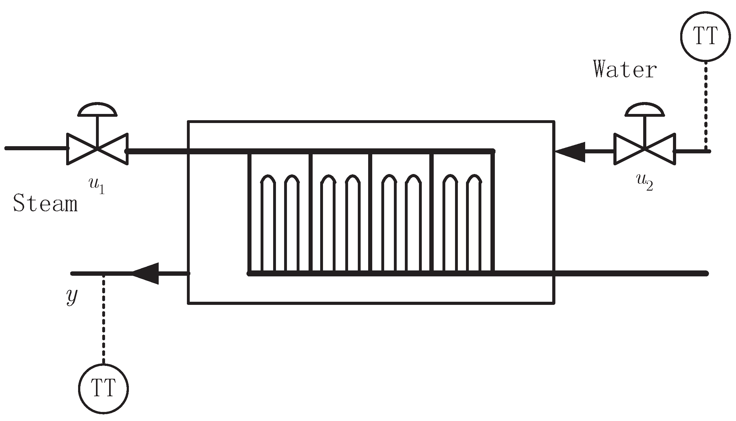
Consider the steam water heat exchanger system in
Figure 1, where the steam flow
and the water flow
are two manipulated variables to control the water temperature
y. The discrete input-output representation of the process is expressed as the following equation.
Figure 1.
The steam water heat exchanger.
Figure 1.
The steam water heat exchanger.
Let
; then the parameter vector to be identified is:
It can be seen from the above equation that the dimension of the parameter vector θ is , but only six of the parameters are non-zeros.
In the identification, the inputs
,
are taken as independent persistent excitation signal sequences with zero mean and unit variances and
as white noise sequences with zero mean and variance
. Let
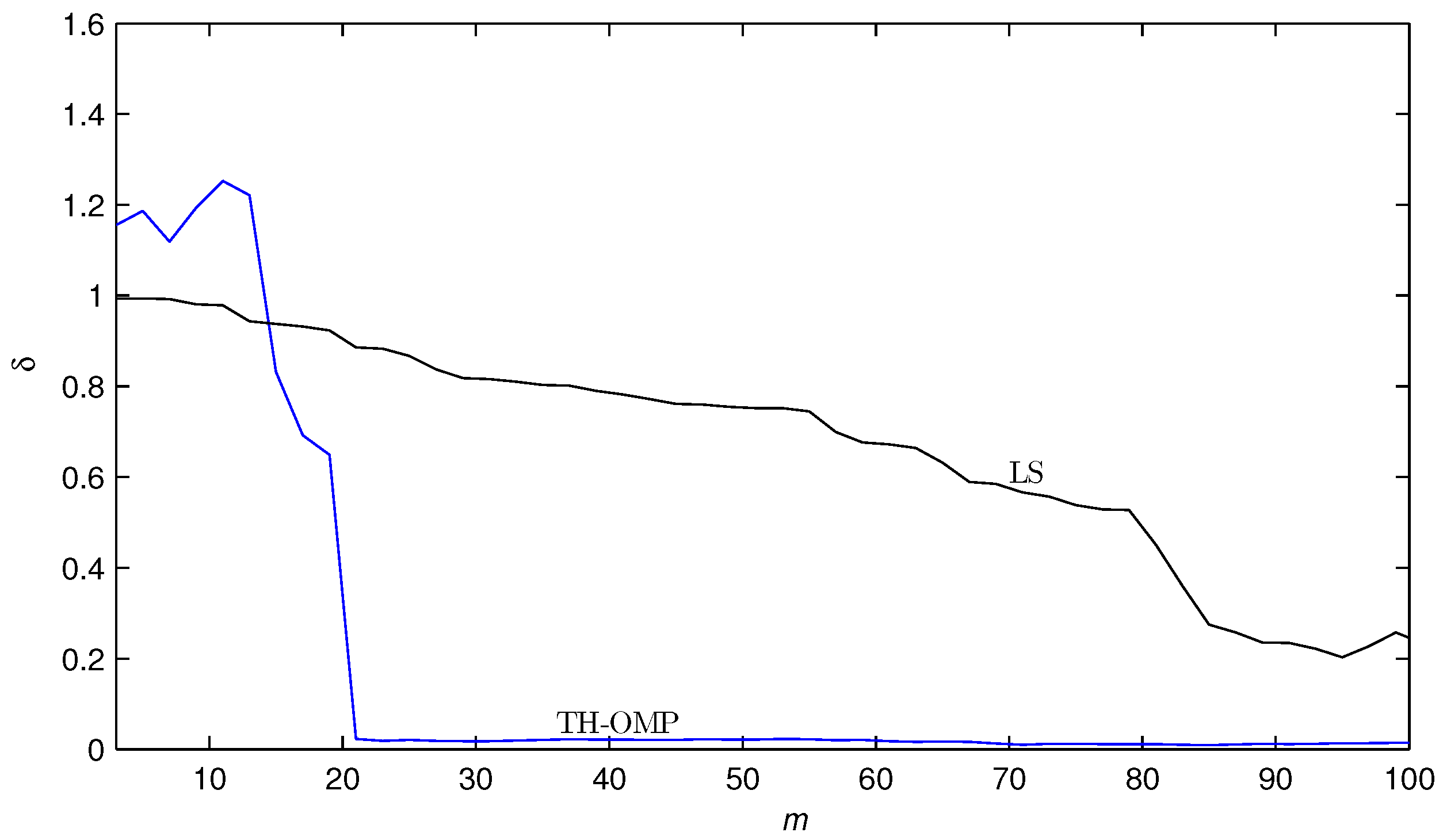
, applying the proposed TH-OMP algorithm and the least squares (LS) algorithm to estimate the system with
m measurements. The parameter estimation errors
versus m are shown in
Figure 2.
From
Figure 2, we can see that under a limited dataset
, the parameter estimation error of the TH-OMP algorithm approaches zero, and the estimation accuracy is much higher than that of the LS algorithm.
Let
; using the TH-OMP algorithm to estimate
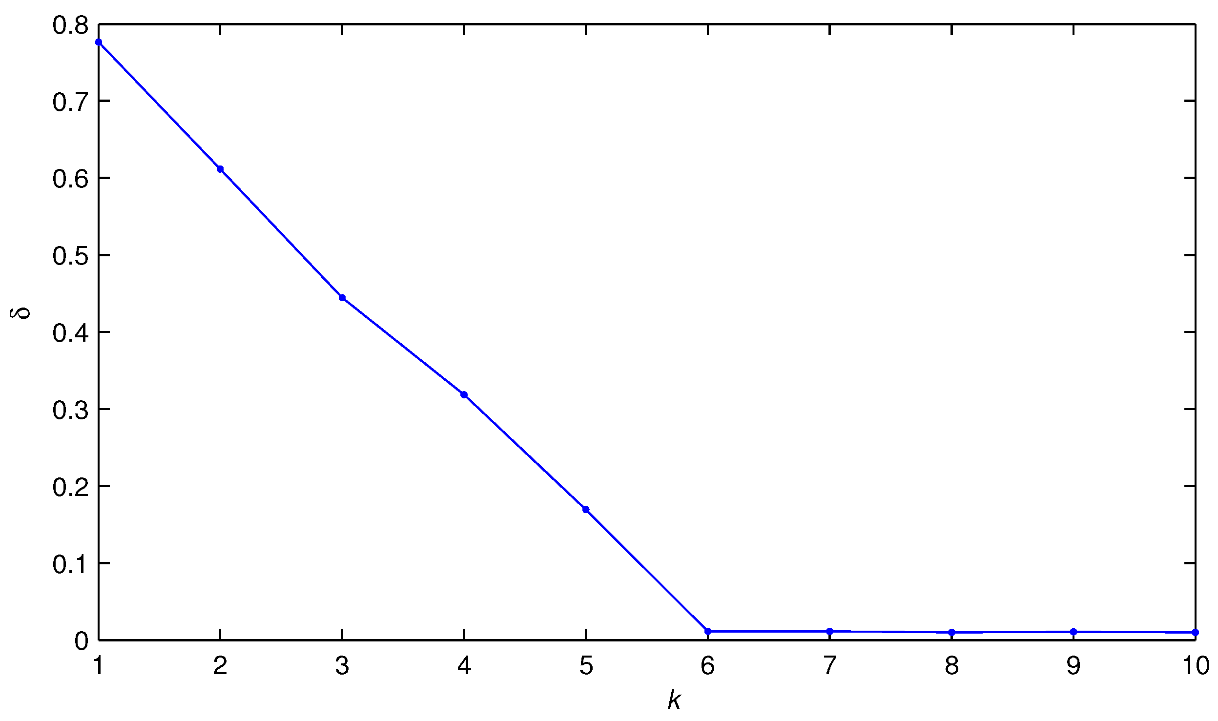
θ, the parameter estimation errors δ
versus iteration
k are shown in
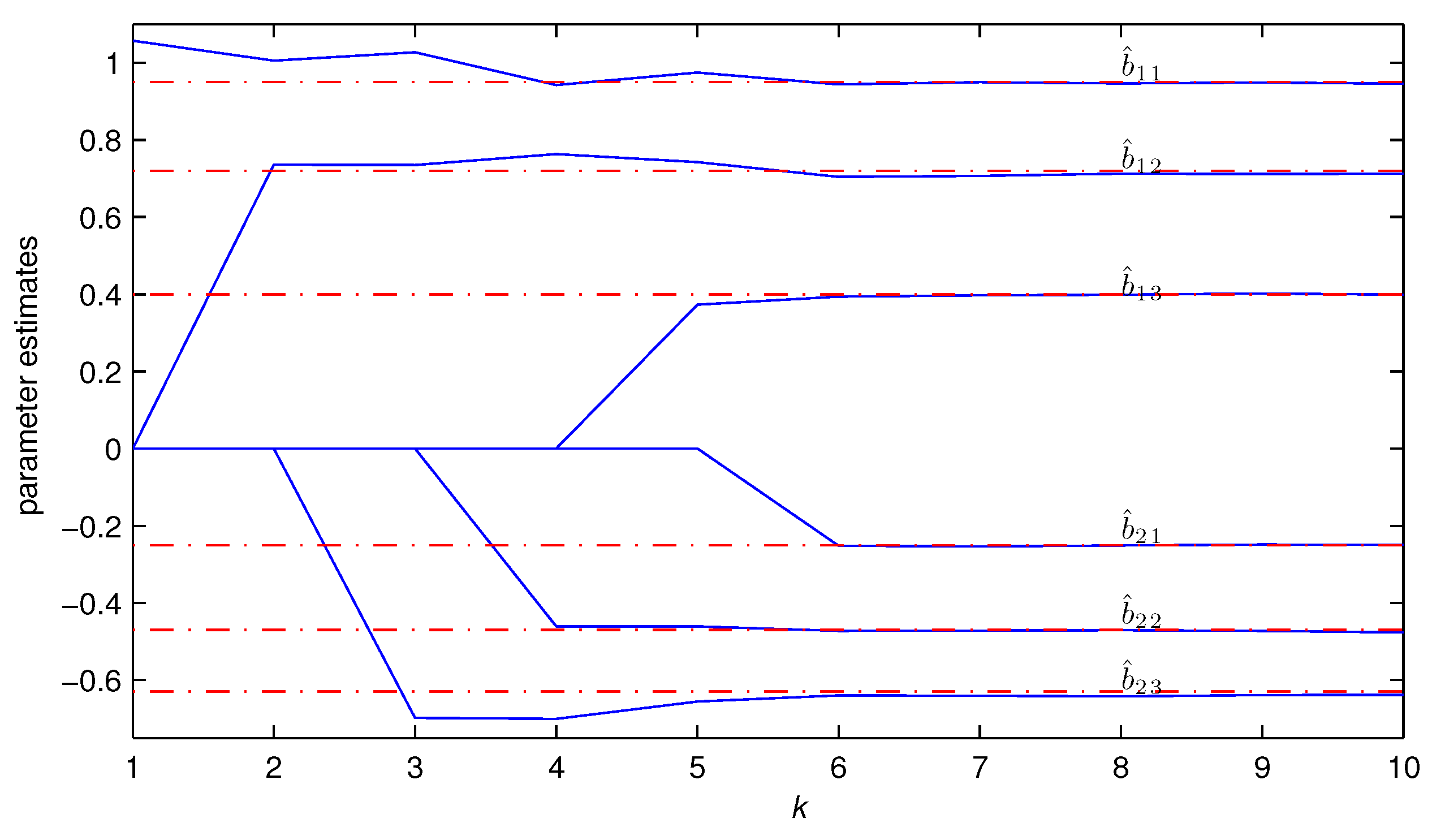
Figure 3; the non-zero parameter estimates
versus iteration
k are shown in
Table 1 and
Figure 4, where the dash dot lines are true parameters and the solid lines are parameter estimates.
Figure 2.
The estimation error δ versus m measurements.
Figure 2.
The estimation error δ versus m measurements.
Figure 3.
The estimation error δ versus iteration k (m = 80, ).
Figure 3.
The estimation error δ versus iteration k (m = 80, ).
Figure 4.
The parameters estimates versus iteration k.
Figure 4.
The parameters estimates versus iteration k.
Table 1.
The estimation error δ versus iteration k (m=80, ).
Table 1.
The estimation error δ versus iteration k (m=80, ).
| k | | | | | | | |
|---|
| 1 | 1.0567 | 0.0000 | 0.0000 | 0.0000 | 0.0000 | 0.0000 | 77.8404 |
| 2 | 1.0056 | 0.7357 | 0.0000 | 0.0000 | 0.0000 | 0.0000 | 61.0813 |
| 3 | 1.0274 | 0.7349 | 0.0000 | −0.6982 | 0.0000 | 0.0000 | 44.8210 |
| 4 | 0.9422 | 0.7635 | 0.0000 | −0.7006 | −0.4604 | 0.0000 | 31.8601 |
| 5 | 0.9748 | 0.7429 | 0.3734 | −0.6551 | −0.4605 | 0.0000 | 16.9639 |
| 6 | 0.9436 | 0.7041 | 0.3936 | −0.6397 | −0.4727 | −0.2522 | 1.3977 |
| 7 | 0.9495 | 0.7071 | 0.3973 | −0.6408 | −0.4715 | −0.2537 | 1.1650 |
| 8 | 0.9466 | 0.7127 | 0.3986 | −0.6422 | −0.4707 | −0.2509 | 0.9755 |
| 9 | 0.9487 | 0.7120 | 0.4022 | −0.6386 | −0.4722 | −0.2490 | 0.8137 |
| 10 | 0.9458 | 0.7129 | 0.3988 | −0.6380 | −0.4766 | −0.2498 | 0.8841 |
| True values | 0.9500 | 0.7200 | 0.4000 | −0.6300 | −0.4700 | −0.2500 | |
After 10 iterations, the estimation error is
, and the estimated parameter vector is:
If we choose
, then we can get the estimated parameter vector as:
It is obvious that the parameter vector θ has only three zero blocks in this example. However, we can see from the above equation that there exist three undesirable parameter estimates , and . Moreover, the three parameter estimates are much smaller than other parameters. Therefore, according to the structure of θ, the parameters , and can be set to zeros. Then, the estimation result is the same as the case when . This implies that even if a too small ϵ is chosen, we can still obtain the effective parameter estimates based on the model structures.
From Equations (15) and (16), we can obtain the orders
and get the time delay estimates as:
From
Figure 2,
Figure 3 and
Figure 4,
Table 1 and Equations (
16) and (
17), we can conclude that the TH-OMP algorithm converges faster than the LS algorithm, can achieve a high estimation accuracy by
K iterations with finite measurements (
) and can effectively estimate the time delay of each channel.


