1. Introduction
Since its discovery by Watson and Crick [
1], the importance of DNA to biology, medicine and human kind has been evident. However, we had to wait some time until it was possible to sequence the DNA bases, which was accomplished by Sanger in the mid-1970s [
2], by detecting small dark bands on a thin gel layer. This method severely constrains the length of the DNA to be sequenced due to the limited resolution of the dark bands. In order to solve this problem, the DNA is first cut in known places by using restriction enzymes, which will divide the DNA at the point where a specific base sequence is found. The resulting sub-sequences, are divided again, this time using a different restriction enzyme, and this process is repeated until the resulting fragments can be divided in random places yielding sub-fragments that are small enough as to provide the complete sequence of bases using Sanger’s method. This process was slow and expensive because every time that a sequence was divided, each resulting subsequence had to be cloned in order to have enough material for the next division. This problem prompted scientists to start dividing sequences in random positions from the beginning, instead of doing it after several divisions, saving time and money [
3]. This method, in turn, created a severe computational problem since there is no information about the order of the fragments. If one starts with many copies of the original problem and the derived fragments are sequenced, then each base of the original problem could appear in several fragments. The sum of the lengths of the fragments divided by the length of the original problem is known as its
coverage. We hope that if we have a large enough coverage, the fragments will overlap in such a way that the sequence at the end of a fragment overlaps with the sequence at the beginning of another one. Hence, in theory, we should be able to use this information to sort the fragments and reconstruct the original DNA sequence.
What really happens is not very simple since, by chance, there are a huge number of false overlaps amongst the fragments. There is also the problem that fragment sequencing is not perfect. Two percent error is common, as well as having fragments that do not belong to the original problem, some due to contamination with DNA foreign to the problem, and others because of the appearance of chimeras from the process of DNA cloning, in which bacteria DNA is used, so that we could get fragments with portions of bacteria DNA. On top of what was said, we have repeats, which are DNA sections that appear tens or hundreds of times one after another (tandem repeats) or in far away parts of the original DNA (interspersed repeats) [
4].
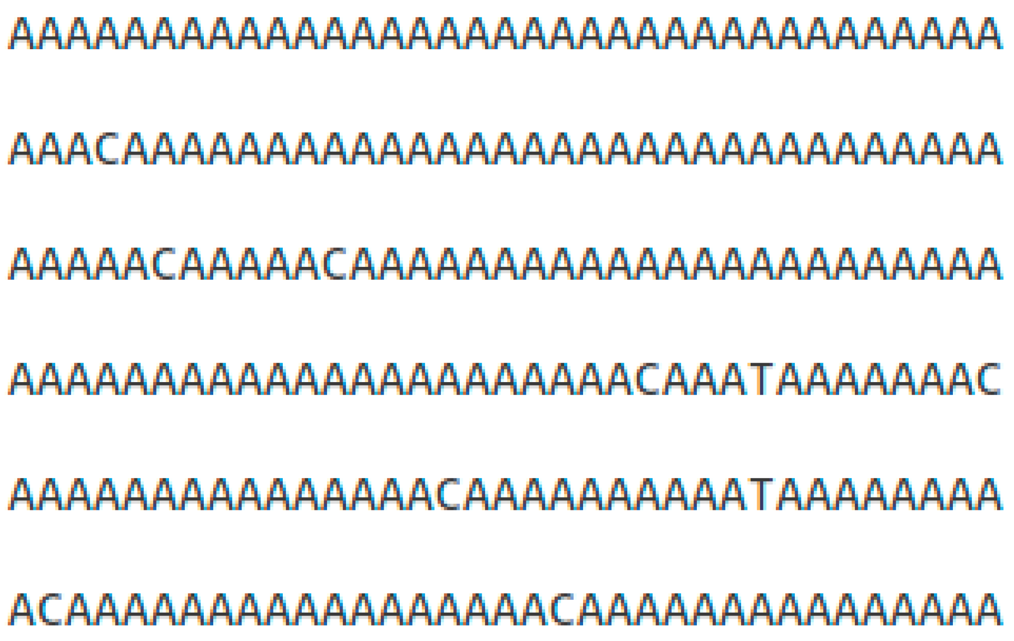
As far as we know, at this point there is no good probabilistic model of DNA. Simple, or relatively simple ones do not explain the repeats. For instance, in the real life problem that we will present later in this paper, there are sequences of A bases that are extremely long.
Figure 1 show some examples of fragments that come from the sample problem that we will use in
Section 4 of this paper and
Table 1 shows the probability that it happens considering that among the total number of fragments, the A bases occurs with probability 0.3249. As can be seen from the figure, the number of times that the A chain occurs in the real data is much larger than the expected value according to a simple probabilistic model. Despite these anomalies and some others, some of the parameters that are used in the assembly of fragments, such as the minimum number of bases that an overlap must have to be considered important, have an empirical basis [
5].
There is also the problem that in real situations, sections of the original DNA problem have no coverage since fragments are obtained by a random process and it is not possible guarantee that there are fragments from every part of the genome under study. This is the reason why the resulting assembly of all fragments is a set of contigs or subsequences and almost never the entire sequence of the problem. It is the job of specialized biologists to fill in the gaps and correct assembly errors made during the automated process.
Figure 1.
Some fragments from the S. aureus strain MW2 problem.
Figure 1.
Some fragments from the S. aureus strain MW2 problem.
Table 1.
Observed frequency on n bases A vs. expected value for p = 0.3249 and 5,324,340 fragments.
Table 1.
Observed frequency on n bases A vs. expected value for p = 0.3249 and 5,324,340 fragments.
| n | Observed | Probability | Expected Value |
|---|
| 15 | 101 | 0.000000475 | 2.528889873 |
| 16 | 74 | 0.000000147 | 0.784225487 |
| 17 | 65 | 0.000000046 | 0.242640081 |
| 18 | 51 | 0.000000014 | 0.074884674 |
| 19 | 40 | 4.32861E−09 | 0.023046972 |
| 20 | 39 | 1.32807E−09 | 0.007071095 |
| 21 | 18 | 4.06052E−10 | 0.002161959 |
| 22 | 28 | 1.23662E−10 | 0.000658416 |
| 23 | 14 | 3.74924E−11 | 0.000199622 |
| 24 | 15 | 1.13089E−11 | 0.000060212 |
| 25 | 22 | 3.3908E−12 | 0.000018054 |
| 26 | 15 | 1.00958E−12 | 0.000005375 |
| 27 | 22 | 2.9809E−13 | 0.000001587 |
| 28 | 11 | 8.71281E−14 | 0.000000464 |
| 29 | 15 | 2.51495E−14 | 0.000000134 |
| 30 | 10 | 7.14487E−15 | 3.80417E−08 |
| 31 | 9 | 1.98796E−15 | 1.05846E−08 |
| 32 | 6 | 5.37563E−16 | 2.86217E−09 |
| 33 | 4 | 1.3946E−16 | 7.42531E−10 |
| 34 | 4 | 3.38757E−17 | 1.80366E−10 |
| 35 | 1 | 7.29107E−18 | 3.88201E−11 |
DNA fragment sequencing technology has continued to advance while costs continue to go down. The original
shotgun technology has been called “long reads” because the fragments would normally have more than 500 bases. Using new technologies, commonly known as Next Generation Sequencing, the cost to sequence a million bases is about $1 [
6]. Unfortunately, the length of the fragments is shorter using this newer technology. Today, 150 bases reads are common with the Illumina sequencers. To compensate for the problems derived from the short size of each fragment, coverage of about 40 is needed instead of a coverage of about 10 in the case of long reads. If we consider the number of fragments to be sequenced with newer technologies, we need to assemble three to four million fragments to sequence a bacterium, while using long reads, only 50,000 fragments were enough. These are really bad news due to the combinatorial nature of the solutions to the problem.
Since the very beginning of DNA fragment sequencing, greedy algorithms have been used; for instance, we pick a random fragment and connect to it the one that has the longest overlap. This process is repeated until no overlapping fragments are available. Nowadays, this technique would be difficult to use, since fragments are too short, which often produces several different fragments with the same overlap size. Another popular technique is the use of De Bruijn graphs [
7]. In order to build these graphs, all possible
k-mers (subsequence of
k consecutive bases) of each fragment are used to find all possible overlaps among them. Using these graphs, several problems can be solved by using heuristics; for instance, given a
k-mer, there might be two parallel paths to other
k-mer, creating what is called a bubble. The bubble is then popped by removing the shortest side or projecting one side onto the other when they have the same length. Short sequences that originate from long ones are eliminated. It is common to use a value of
k close to 20 in order to obtain the
k-mers.
An approach based on genetic algorithm optimization was suggested by Parsons in 1993 [
8]. Later, other scientists applied similar metaheuristics [
9,
10,
11,
12], but their results were based on very small benchmarks, the largest had about 1000 fragments, and even though results were improving slowly, they were still far from real problems, including the long reading ones, with tens of thousands of fragments. In 2013, a reduction from fragment DNA sequencing to the Traveling Salesman Problem (TSP) was used [
13]. Taking advantage of formal heuristics and algorithms for the TSP, optimal values were found for the most commonly used benchmarks, and, for the first time, a real life problem was solved using optimization.
The remainder of this paper is organized as follows:
Section 2 provides the basic ideas on the use of graph theory for the solution of DNA sequencing problems;
Section 3 explains those algorithms that are necessary to tackle the problem;
Section 4 illustrates the use of our algorithms on real life problem benchmarks; and, in
Section 5, we give our conclusions and future work.
4. Experiments
In order to test our algorithms, we used several benchmarks that are available for use by researchers [
19]. We selected the benchmarks of
S. aureus MW2 with short reads. The benchmarks that we used have the following number of fragments: 2,278,504, 730,201, 298,194, 89,718 and 22,447. From now on, we will refer to each one of these problems by its number of fragments. In order to have something to compare our results to, we ran the Edena assembler using the same data,
Table 4. This comparison has some limitations due to the fact that Edena uses a series of heuristics in order to refine its solution, by eliminating
contigs that have no real meaning, while our results are those directly generated by our algorithms with no refinement. Refining the raw results from our algorithms might be part of our future research.
Table 4.
Edena benchmark results.
Table 4.
Edena benchmark results.
| | Problem |
|---|
| Fragments | 22,448 | 89,718 | 298,194 | 730,201 | 2,278,504 |
| Contigs Obtained | 186 | 258 | 575 | 837 | 2046 |
| Total Number of Bases | 26,284 | 102,684 | 314,120 | 788,198 | 2,526,278 |
| Contigs Found | Contigs Found | 184 | 256 | 565 | 823 | 1920 |
| % | 98.9 | 99.2 | 98.3 | 98.3 | 93.8 |
| Bases Found | 26,024 | 102,249 | 310,965 | 777,583 | 2,463,563 |
| % | 99 | 99.6 | 99 | 98.7 | 97.5 |
| N50 | 188 | 1247 | 2911 | 4132 | 5250 |
| Average Length | 141.4 | 399.4 | 550.4 | 944.8 | 1283.10 |
| Minimum Length | 52 | 52 | 52 | 52 | 52 |
| Maximum Length | 880 | 7295 | 10,985 | 20,521 | 20,579 |
| Contigs not Found | Contigs not Found | 2 | 2 | 10 | 14 | 126 |
| % | 1.1 | 0.8 | 1.7 | 1.7 | 6.2 |
| Bases not Found | 260 | 435 | 3155 | 10,615 | 62,715 |
| % | 1 | 0.4 | 1 | 1.3 | 2.5 |
| N50 | NA | NA | NA | NA | 5599 |
| Average Length | 130 | 217.5 | 315.5 | 758.2 | 497.7 |
| Minimum Length | 99 | 99 | 56 | 56 | 52 |
| Maximum Length | 161 | 336 | 2521 | 5941 | 18,158 |
From each benchmark, we took only the fragment file in FASTA format, and from it we computed the overlaps among all fragments considering that reverse-complement fragments are also independent fragments (In the original benchmarks, there is a file of overlaps where reverse-complements are not considered as independent fragments). To compute overlaps, we used a
trie (prefix tree). The computed overlaps are all larger than 20 bases. From these overlaps other sets of test data were obtained: one discarding redundant overlaps because of transitivity, and the other one, computing the MST. In all of the cases, the minimum agreement in Algorithm 5 was 4. The
contigs obtained in each experiment were searched in the complete genome [
20].
In Experiment 1, we used all of the overlaps larger than 20 bases and executed Algorithm 1 for the two objective functions. The results are presented in
Table 5,
Table 6 and
Table 7.
Table 5.
Experiments summary.
Table 5.
Experiments summary.
| | Problem |
|---|
| Algorithm | | Fragments | 22,448 | 89,718 | 298,194 | 730,201 | 2,278,504 |
| Edena | Edena | Contigs Found | 184 | 256 | 565 | 823 | 1920 |
| % | 98.9 | 99.2 | 98.3 | 98.3 | 93.8 |
| Bases Found | 26,024 | 102,249 | 310,965 | 777,583 | 2,463,563 |
| % | 99 | 99.6 | 99 | 98.7 | 97.5 |
| Algorithm 1 | F1 Objective Function, all Overlaps. | Contigs Found | 74 | 101 | 149 | 204 | 480 |
| % | 90.2 | 88.6 | 91.4 | 91.1 | 94.1 |
| Bases Found | 15,822 | 70,250 | 206,826 | 463,582 | 1,102,152 |
| % | 81.8 | 83 | 86.1 | 83.9 | 83.4 |
| Algorithm 1 | F2 Objective Function, all Overlaps | Contigs found | 74 | 102 | 146 | 189 | 450 |
| % | 90.2 | 89.5 | 89.6 | 84.4 | 88.2 |
| Bases found | 15,515 | 70,843 | 189,927 | 369,001 | 931,343 |
| % | 81.5 | 83.8 | 79 | 66.8 | 69.9 |
| Algorithm 1 | F1 Objective Function, no Transitive overlaps | Contigs found | 74 | 102 | 149 | 204 | 481 |
| % | 90.2 | 89.5 | 91.4 | 91.1 | 93.9 |
| Bases found | 15,806 | 71,652 | 206,826 | 462,774 | 1,103,587 |
| % | 83.7 | 84.6 | 86.1 | 83.9 | 82.7 |
| Algorithm 1 | F2 Objective Function, no Transitive Overlaps | Contigs found | 75 | 103 | 142 | 181 | 417 |
| % | 91.5 | 90.4 | 87.1 | 80.8 | 81.4 |
| Bases found | 15,599 | 72,245 | 174,244 | 320,502 | 791,376 |
| % | 84 | 85.4 | 72.5 | 58.1 | 58.9 |
| Algorithm 1 | F1 Objective Function, MST | Contigs found | 304 | 1827 | 5980 | 15,443 | 46,187 |
| % | 91 | 97 | 98.4 | 98.9 | 95.7 |
| Bases found | 35,980 | 256,641 | 815,994 | 2,081,306 | 6,208,258 |
| % | 89.8 | 96.6 | 98.1 | 98.7 | 93.9 |
| Algorithm 5 | F1 Objective function, no Transitive Edges | Contigs found | 74 | 102 | 150 | 205 | 480 |
| % | 90.2 | 88.7 | 91.5 | 91.1 | 94.1 |
| Bases found | 15,822 | 70,318 | 206,927 | 463,684 | 1,102,152 |
| % | 81.8 | 83 | 86.1 | 83.9 | 83.4 |
Table 6.
Algorithm 1, F1 objective function, all overlaps.
Table 6.
Algorithm 1, F1 objective function, all overlaps.
| | Problem |
|---|
| Fragments | 22,448 | 89,718 | 298,194 | 730,201 | 2,278,504 |
| Contigs Obtained | 82 | 114 | 163 | 224 | 510 |
| Total Number of Bases | 19,343 | 84,659 | 240,314 | 552,408 | 1,321,969 |
| Contigs Found | Contigs Found | 74 | 101 | 149 | 204 | 480 |
| % | 90.2 | 88.6 | 91.4 | 91.1 | 94.1 |
| Bases Found | 15,822 | 70,250 | 206,826 | 463,582 | 1,102,152 |
| % | 81.8 | 83 | 86.1 | 83.9 | 83.4 |
| N50 | 360 | 1614 | 3326 | 4937 | 4499 |
| Average Length | 213.8 | 695.5 | 1388.10 | 2272.50 | 2296.20 |
| Minimum Length | 54 | 58 | 54 | 62 | 53 |
| Maximum Length | 882 | 7261 | 10,943 | 22,745 | 24,396 |
| Contigs not Found | Contigs not Found | 8 | 13 | 14 | 20 | 30 |
| % | 9.8 | 11.4 | 8.6 | 8.9 | 5.9 |
| Bases not Found | 3521 | 14,409 | 33,488 | 88,826 | 219,817 |
| % | 18.2 | 17 | 13.9 | 16.1 | 16.6 |
| N50 | 758 | 2308 | 3954 | 7258 | 11,798 |
| Average Length | 440.1 | 1108.40 | 2392.00 | 4441.30 | 7327.20 |
| Minimum Length | 95 | 95 | 95 | 181 | 255 |
| Maximum Length | 826 | 3703 | 6809 | 9542 | 23,614 |
Table 7.
Algorithm 1, F2 objective function, all overlaps.
Table 7.
Algorithm 1, F2 objective function, all overlaps.
| | Problem |
|---|
| Fragments | 22,448 | 89,718 | 298,194 | 730,201 | 2,278,504 |
| Contigs Obtained | 82 | 114 | 163 | 224 | 510 |
| Total Number of Bases | 19,028 | 84,584 | 240,280 | 552,509 | 1,331,757 |
| Contigs Found | Contigs Found | 74 | 102 | 146 | 189 | 450 |
| % | 90.2 | 89.5 | 89.6 | 84.4 | 88.2 |
| Bases Found | 15,515 | 70,843 | 189,927 | 369,001 | 931,343 |
| % | 81.5 | 83.8 | 79 | 66.8 | 69.9 |
| N50 | 356 | 1527 | 3184 | 4298 | 4201 |
| Average Length | 209.7 | 694.5 | 1300.90 | 1952.40 | 2069.70 |
| Minimum Length | 54 | 58 | 54 | 59 | 53 |
| Maximum Length | 882 | 7261 | 10,943 | 21,185 | 16,135 |
| Contigs not Found | Contigs not Found | 8 | 12 | 17 | 35 | 60 |
| % | 9.8 | 10.5 | 10.4 | 15.6 | 11.8 |
| Bases not Found | 3513 | 13,741 | 50,353 | 183,508 | 400,414 |
| % | 18.5 | 16.2 | 21 | 33.2 | 30.1 |
| N50 | 758 | 2308 | 6336 | 7620 | 9472 |
| Average Length | 439.1 | 1145.10 | 2961.90 | 5243.10 | 6673.60 |
| Minimum Length | 95 | 96 | 103 | 181 | 251 |
| Maximum Length | 826 | 3703 | 7626 | 22,745 | 24,396 |
From the DNA fragment assembly point of view, we are interested in large contigs with no errors. The most important elements to be computed are the number of bases and the contigs that were found in the complete genome, as well as the mean length of each contig. When we compare the results obtained by Algorithm 1 for F1 and F2 using all overlaps, we find that F1 is a little bit better than F2, except in the number of bases found for problem 89,718. In terms of multi objective function optimization, the solution obtained for F1 is not enough to dominate the solution obtained by F2, but since it is better in most of the test, we can say that it is almost dominant. In the other experiments, we find a similar situation, where F1 is almost dominant with respect to F2.
For Experiment 2, we excluded transitive overlaps and used Algorithm 1 for
F1 and
F2. The results are given in
Table 5,
Table 8 and
Table 9.
Table 8.
Algorithm 1, F1 objective function, no transitive overlaps.
Table 8.
Algorithm 1, F1 objective function, no transitive overlaps.
| | Problem |
|---|
| Fragments | 22,448 | 89,718 | 298,194 | 730,201 | 2,278,504 |
| Contigs Obtained | 82 | 114 | 163 | 224 | 512 |
| Total Number of Bases | 18,879 | 84,646 | 240,314 | 551,600 | 1,333,881 |
| Contigs Found | Contigs Found | 74 | 102 | 149 | 204 | 481 |
| % | 90.2 | 89.5 | 91.4 | 91.1 | 93.9 |
| Bases Found | 15,806 | 71,652 | 206,826 | 462,774 | 1,103,587 |
| % | 83.7 | 84.6 | 86.1 | 83.9 | 82.7 |
| N50 | 360 | 1527 | 3326 | 4937 | 4499 |
| Average Length | 213.6 | 702.5 | 1388.10 | 2268.50 | 2294.40 |
| Minimum Length | 54 | 58 | 54 | 62 | 53 |
| Maximum Length | 882 | 7261 | 10,943 | 22,745 | 24,396 |
| Contigs not Found | Contigs not Found | 8 | 12 | 14 | 20 | 31 |
| % | 9.8 | 10.5 | 8.6 | 8.9 | 6.1 |
| Bases not Found | 3073 | 12,994 | 33,488 | 88,826 | 230,294 |
| % | 16.3 | 15.4 | 13.9 | 16.1 | 17.3 |
| N50 | 539 | 2308 | 3954 | 7258 | 11,657 |
| Average Length | 384.1 | 1082.80 | 2392.00 | 4441.30 | 7428.80 |
| Minimum Length | 95 | 95 | 95 | 181 | 255 |
| Maximum Length | 826 | 3703 | 6809 | 9542 | 23,614 |
In general, we found that
F1 is better than
F2 without dominating it. Comparing the results where transitive overlaps are excluded (
Table 8 and
Table 9 or
Table 5) to those where they are not (
Table 6 and
Table 7 or
Table 5), we can see that the results are similar for
F1, hence it is not clear whether it is better to exclude or not to exclude transitive overlaps. There is, however, an obvious advantage of excluding transitive overlaps, which is that the problem size is reduced and requires less computational resources. So, our recommendation is to exclude transitive overlaps.
Comparing our results so far to Edena, we find out that we obtained fewer correct bases and more contigs that are not in the genome, but the length of our contigs is better.
Table 9.
Algorithm 1, F2 objective function, no transitive overlaps.
Table 9.
Algorithm 1, F2 objective function, no transitive overlaps.
| | Problem |
|---|
| Fragments | 22,448 | 89,718 | 298,194 | 730,201 | 2,278,504 |
| Contigs Obtained | 82 | 114 | 163 | 224 | 512 |
| Total Number of Bases | 18,579 | 84,571 | 240,265 | 551,701 | 1,343,637 |
| Contigs Found | Contigs Found | 75 | 103 | 142 | 181 | 417 |
| % | 91.5 | 90.4 | 87.1 | 80.8 | 81.4 |
| Bases Found | 15,599 | 72,245 | 174,244 | 320,502 | 791,376 |
| % | 84 | 85.4 | 72.5 | 58.1 | 58.9 |
| N50 | 356 | 1527 | 2984 | 3910 | 4135 |
| Average Length | 208 | 701.4 | 1227.10 | 1770.70 | 1897.80 |
| Minimum Length | 54 | 58 | 54 | 59 | 53 |
| Maximum Length | 882 | 7,261 | 10,943 | 10,648 | 16,135 |
| Contigs not Found | Contigs not Found | 7 | 11 | 21 | 43 | 95 |
| % | 8.5 | 9.6 | 12.9 | 19.2 | 18.6 |
| Bases not Found | 2980 | 12,326 | 66,021 | 231,199 | 552,261 |
| % | 16 | 14.6 | 27.5 | 41.9 | 41.1 |
| N50 | 539 | 2308 | 6336 | 8135 | 7554 |
| Average Length | 425.7 | 1120.50 | 3143.90 | 5376.70 | 5813.30 |
| Minimum Length | 95 | 96 | 103 | 181 | 251 |
| Maximum Length | 826 | 3703 | 10,648 | 22,745 | 24,396 |
Table 10.
Algorithm 1, F1 objective function, Minimum Spanning Tree (MST).
Table 10.
Algorithm 1, F1 objective function, Minimum Spanning Tree (MST).
| | Problem |
|---|
| Fragments | 22,448 | 89,718 | 298,194 | 730,201 | 2,278,504 |
| Contigs Obtained | 334 | 1883 | 6080 | 15,618 | 48,263 |
| Total Number of Bases | 40,076 | 265,584 | 831,449 | 2,109,070 | 6,613,747 |
| Contigs Found | Contigs Found | 304 | 1827 | 5980 | 15,443 | 46,187 |
| % | 91 | 97 | 98.4 | 98.9 | 95.7 |
| Bases Found | 35,980 | 256,641 | 815,994 | 2,081,306 | 6,208,258 |
| % | 89.8 | 96.6 | 98.1 | 98.7 | 93.9 |
| N50 | 135 | 165 | 154 | 153 | 153 |
| Average Length | 118.4 | 140.5 | 136.5 | 134.8 | 134.4 |
| Minimum Length | 62 | 62 | 61 | 57 | 57 |
| Maximum Length | 446 | 660 | 747 | 894 | 1152 |
| Contigs not Fund | Contigs not Found | 30 | 56 | 100 | 175 | 2076 |
| % | 9 | 3 | 1.6 | 1.1 | 4.3 |
| Bases not Found | 4096 | 8943 | 15,455 | 27,764 | 405,489 |
| % | 10.2 | 3.4 | 1.9 | 1.3 | 6.1 |
| N50 | 154 | 199 | 198 | 194 | 245 |
| Average Length | 136.5 | 159.7 | 154.6 | 158.7 | 195.3 |
| Minimum Length | 64 | 65 | 65 | 64 | 63 |
| Maximum Length | 362 | 481 | 481 | 493 | 1130 |
In Experiment 3, we obtained the Minimum Spanning Tree (MST) from all overlaps using our version of Kruskal’s algorithm. We only show the results for
F1 (
Table 5 and
Table 10). In this case, we were able to find much more bases in the genome than in previous experiments, including Edena, but the size of our
contigs is small. There appears to be a tradeoff between the number of bases that can be found and
contig length.
In other experiments, we used Algorithm 4 without transitive overlaps, obtaining similar results to those of Algorithm 1 for
F1 (
F1 was again better than
F2). Analyzing the
contigs obtained by the algorithm, we found that if the
contig is split at the edge that joins the cycle with the path, we have a better chance of finding both
contigs. Therefore, we modified Algorithm 4 making d(v) = 0 in Step 2.2.1.1 and repeated Experiment 4 without transitive overlaps. In this case, the objective function
F1 was better than
F2 without being dominant. These results are given in
Table 5 and
Table 11.
Table 11.
Algorithm 5, F1 objective function, no transitive edges.
Table 11.
Algorithm 5, F1 objective function, no transitive edges.
| | Problem |
|---|
| Fragments | 22,448 | 89,718 | 298,194 | 730,201 | 2,278,504 |
| Contigs Obtained | 82 | 115 | 164 | 225 | 510 |
| Total Number of Bases | 19,343 | 84,727 | 240,415 | 552,510 | 1,321,969 |
| Contigs Found | Contigs Found | 74 | 102 | 150 | 205 | 480 |
| % | 90.2 | 88.7 | 91.5 | 91.1 | 94.1 |
| Bases Found | 15,822 | 70,318 | 206,927 | 463,684 | 1,102,152 |
| % | 81.8 | 83 | 86.1 | 83.9 | 83.4 |
| N50 | 360 | 1614 | 3326 | 4937 | 4499 |
| Average Length | 213.8 | 689.4 | 1379.50 | 2261.90 | 2296.20 |
| Minimum Length | 54 | 58 | 54 | 62 | 53 |
| Maximum Length | 882 | 7261 | 10,943 | 22,745 | 24,369 |
| Contigs not Found | Contigs not Fund | 8 | 13 | 14 | 20 | 30 |
| % | 9.8 | 11.3 | 8.5 | 8.9 | 5.9 |
| Bases not Found | 3521 | 14,409 | 33,488 | 88,826 | 219,817 |
| % | 18.2 | 17 | 13.9 | 16.1 | |
| N50 | 758 | 2308 | 3954 | 7258 | 11,798 |
| Average Length | 440.1 | 1108.40 | 2392.00 | 4441.30 | 7327.20 |
| Minimum Length | 95 | 95 | 95 | 181 | 255 |
| Maximum Length | 826 | 3703 | 6809 | 9542 | 23,614 |
In an analysis of those contigs that were not found in the genome, we considered the possibility of splitting them in two or more pieces hoping that all of them could be found. There are few cases in which contigs should be divided; in problem 730,201, using the modified Algorithm 4 with F1, there were 513 contigs from which 414 were found directly, 76 were split in two to be found, 14 in three, 10 in four or more pieces, and two produced pieces that were too small to be considered. With appropriate rules, it should be possible to find the correct split points in most of the cases, as other assemblers do. We also analyzed residual paths, after removing paths of maximum length, from which we considered the possibility of recovering several long contings, which we will do in the future.
5. Conclusions and Future Work
In order to assemble DNA, it is possible to use traditional graph theory concepts being careful to use only linear algorithms due to the large amount of data that is handled. With this idea, we developed a constant time heap, appropriate for this particular case (and maybe to other cases as well), which allowed us to reduce the time complexity of other algorithms, such as Prim’s and Kruskal’s, making them linear.
If we compare the results of the objective functions F1 and F2, even though one does not dominate over the other, better results are obtained using F1, hence we recommend its use. We also recommend the removal of transitive overlaps because of resource reduction considerations, even though the results of the assembly are almost the same for function F1. The use of the MST considerably improves the number of correct bases, but the contigs obtained in this way are too small. It can be seen from the experiments that there is a tradeoff between contig length and the number of bases detected. Comparing our results to those of Edena is not completely objective since we do not apply heuristics after the algorithms are executed in order to refine the solutions, but Edena (as well as the Velvet assembler) do so intensively. In any case, compared to Edena, our method produced, in some cases, less bases but longer contigs, while, in other cases, we found more bases, but shorter contigs, especially when using MST. Therefore, the problem must be considered as a multi objective optimization, with an objective function that is able to maximize the number of mean contig length, giving the user a Pareto Front from which he can obtain the most convenient solution according to his particular criteria.
Our future work includes:
Developing rules to split contigs in such a way that most of the pieces can be found.
Attempting to recover other contigs after extracting the longest ones.
Implementing a solution to DNA fragment assembly as a multi objective optimization problem.


