Article

A Family of Newton Type Iterative Methods for Solving Nonlinear Equations

1
School of Mathematics and Physics, Bohai University, Jinzhou 121013, China
2
College of Engineering, Bohai University, Jinzhou 121013, China
*
Author to whom correspondence should be addressed.
Algorithms 2015, 8(3), 786-798; https://0-doi-org.brum.beds.ac.uk/10.3390/a8030786
Submission received: 9 July 2015 / Revised: 14 September 2015 / Accepted: 15 September 2015 / Published: 22 September 2015
(This article belongs to the Special Issue Numerical Algorithms for Solving Nonlinear Equations and Systems)

Abstract

:
In this paper, a general family of n-point Newton type iterative methods for solving nonlinear equations is constructed by using direct Hermite interpolation. The order of convergence of the new n-point iterative methods without memory is 2 n requiring the evaluations of n functions and one first-order derivative in per full iteration, which implies that this family is optimal according to Kung and Traub’s conjecture (1974). Its error equations and asymptotic convergence constants are obtained. The n-point iterative methods with memory are obtained by using a self-accelerating parameter, which achieve much faster convergence than the corresponding n-point methods without memory. The increase of convergence order is attained without any additional calculations so that the n-point Newton type iterative methods with memory possess a very high computational efficiency. Numerical examples are demonstrated to confirm theoretical results.

Graphical Abstract

1. Introduction

Solving nonlinear equations by iterative methods have been of great interest to numerical analysts. The most famous one-point iterative method is probably Newton’s Equation [1]: x k + 1 = x k - f ( x k ) / f ( x k ) , which converges quadratically. However, the condition f ( x ) 0 in a neighborhood of the required root is severe indeed for convergence of Newton method, which restricts its applications in practical. For resolving this problem, Wu in [2] proposed the following one-point iterative method
x k + 1 = x k - f ( x k ) λ f ( x k ) + f ( x k )
where λ R , 0 < λ < + and λ is chosen such that the corresponding function values λ f ( x k ) and f ( x k ) have the same signs. This method converges quadratically under the condition λ f ( x k ) + f ( x k ) 0 , while f ( x k ) = 0 in some points is permitted. Wang and Zhang in [3] obtained the error equation of the Equation (1) as follows
e k + 1 = ( c 2 + λ ) e k 2 + O ( e k 3 )
where e k = x k - a , c k = ( 1 / k ! ) f ( k ) ( a ) / f ( a ) , k = 2 , 3 , and a is the root of the nonlinear equation f ( x ) = 0 .
The convergence order and computational efficiency of the one-point iterative methods are lower than multipoint iterative methods. Multipoint iterative methods can overcome theoretical limits of one-point methods concerning the convergence order and computational efficiency. In recent years, many multipoint iterative methods have been proposed for solving nonlinear equations, see [4,5,6,7,8,9,10,11,12,13,14,15,16,17,18]. Wang and Liu in [4] developed the following eighth-order iterative method without memory by Hermite interpolation methods
y k = x k - f ( x k ) f ( x n ) z k = y k - f ( y k ) 2 f [ y k , x k ] - f ( x k ) x k + 1 = z k - f ( z k ) N ( x k , y k , z k )
where N ( x k , y k , z k ) = f [ z k , y k ] + 2 f [ z k , x k ] - 2 f [ y k , x k ] + f [ y k , x k , x k ] ( y k - z k ) . Using the same strategy, Kou in [5] presented a family of eighth-order iterative method without memory. The Equation (3) is a special case of the Kou’s method. Petković in [6] claimed a general class of optimal n-point methods without memory by Hermite interpolation methods, which have the order of convergence 2 n and require evaluations of n functions and one first-order derivative. The Equation (3) is a special case of the Petković’s n-point Method for n = 3 . But, the Petković’s n-point method gives no specific iterative scheme and error relation for n 4 . In this paper, we construct a class of n-point iterative methods with and without memory by Hermite interpolation methods and give the specific iterative scheme and error relation for all n 2 .
This paper is organized as follows. In Section 2, based on Wu’s Equation [2] and Petković’s n-point Equation [6], we derive a family of n-point iterative methods without memory for solving nonlinear equations. We prove that the order of convergence of the n-point methods without memory is 2 n requiring the evaluations of n functions and one first-order derivative in per full iteration. Kung and Traub in [7] conjectured that a multipoint iteration without memory based on n functional evaluations could achieve an optimal convergence of order 2 n - 1 . The new methods without memory agree with the conjecture. Further accelerations of convergence speed are attained in Section 3. A family of n-point iterative methods with memory is obtained by using a self-accelerating parameter in per full iteration. This self-accelerating parameter is calculated using information available from the current and previous iterations. Numerical examples are given in Section 4 to confirm theoretical results.

2. The Optimal Fourth-, Eighth- and 2 n th Order Iterative Methods

Based on Wu’s Equation [2] and Petković’s n-point methods [6], we derive a general optimal 2 n th order family and write it in the following form:
y k , 1 = y k , 0 - f ( y k , 0 ) λ f ( y k , 0 ) + f ( y k , 0 ) y k , 2 = y k , 1 - f ( y k , 1 ) f [ y k , 1 , y k , 0 ] + f [ y k , 1 , y k , 0 , y k , 0 ] ( y k , 1 - y k , 0 ) y k , n = y k , n - 1 - f ( y k , n - 1 ) N ( y k , n - 1 , y k , n - 2 , y k , 1 , y k , 0 )
where N ( y k , n - 1 , y k , n - 2 , , y k , 1 , y k , 0 ) = f [ y k , n - 1 , y k , n - 2 ] + + f [ y k , n - 1 , y k , n - 2 , , y k , 1 , y k , 0 , y k , 0 ] ( y k , n - 1 - y k , n - 2 ) ( y k , n - 1 - y k , 0 ) , y k , 0 = x k , λ R is a constant and k being the iteration index. The entries y k , 0 , y k , n are approximations with the associated error e k , j = y k , j - a ( j = 0 , 1 , , n ) .
Using the Taylor series and symbolic computation in the programming package Mathematica, we can find the order of convergence and the asymptotic error constant (AEC) of the n-point methods Equation (4) for n = 1 , n = 2 and n = 3 , respectively. For simplicity, we sometimes omit the iteration index n and write e instead of e k . The approximation x k + 1 to the root a will be denoted by x ^ . Regarding Equation (4), let us define x = y k , 0 , y = y k , 1 , z = y k , 2 , e = x - a , d = y - a , p = z - a , e 1 = x ^ - a .
The following abbreviations are used in the program.
ck = f ( k ) ( a ) / ( k ! f ( a ) ) , e = x - a , d = y - a , p = z - a , el = x ^ - a , fx = f ( y k , 0 ) , fy = f ( y k , 1 )
dfx = f ( y k , 0 ) , fxxy = f [ y k , 0 , y k , 0 , y k , 1 ] , fla = f ( a ) , fyz = f [ y k , 1 , y k , 2 ] , fxz = f [ y k , 0 , y k , 2 ] ,
fz = f ( y k , 2 ) , L = λ , fzxx = f [ y k , 2 , y k , 0 , y k , 0 ] , fxy = f [ y k , 0 , y k , 1 ] , fzxxy = f [ y k , 2 , y k , 0 , y k , 0 , y k , 1 ] .
Program (written in Mathematica)
fx=fla*(e+c2*e^2+c3*e^3+c4*e^4+c5*e^5+c6*e^6+c7*e^7+c8*e^8);
dfx=D[fx,e];
t=Series[fx/(L*fx+dfx),{e,0,8}];
d=Series[e-t,{e,0,8}]//Simplify
fy=Series[fla*(d+c2*d^2+c3*d^3+c4*d^4),{e,0,8}];
fxy=Series[(fy-fx)/(d-e),{e,0,8}];
z=Series[d-fy/(2*fxy-dfx),{e,0,8}]//Simplify
fz=Series[fla*(z+c2*z^2),{e,0,8}];
fyz=Series[(fy-fz)/(d-z),{e,0,8}];
fxz=Series[(fx-fz)/(e-z),{e,0,8}];
fxxy=Series[(dfx-fxy)/(e-d),{e,0,8}];
fzxx=Series[(dfx-fxz)/(e-z),{e,0,8}];
fzxxy=Series[(fzxx-fxxy)/(z-d),{e,0,8}];
fzxy=Series[(fxz-fyz)/(e-d),{e,0,8}];
e1=Series[z-fz/(fyz+fzxy*(z-d)+fzxxy*(z-e)*(z-d)),{e,0,8}]//Simplify
Out [ d ] = ( c 2 + L ) e 2 + O [ e ] 3
Out [ z ] = ( c 2 + L ) ( c 2 2 - c 3 + c 2 L ) e 4 + O [ e ] 5
Out [ el ] = ( c 2 + L ) 2 ( c 2 2 - c 3 + c 2 L ) ( c 2 3 - c 2 c 3 + c 4 + c 2 2 L ) e 8 + O [ e ] 9
We obtain the asymptotic error constants of n-point methods Equation (4) with n = 1 , 2 , 3 . Altogether, we can state the following theorem.
Theorem 1. Let I be an open interval and a I a simple zero point of a sufficiently differentiable function f : I R . Then the new method defined by Equation (4) ( n = 2 ) is fourth order, and satisfies the error equation
e k + 1 = ( c 2 + λ ) d 2 e k 4 + O ( e k 5 )
the Equation (4) ( n = 3 ) is eighth-order and satisfies the error equation
e k + 1 = ( c 2 + λ ) 2 d 3 e k 8 + O ( e k 9 )
where e k = x k - a , d 0 = 1 , d 1 = 1 , d 2 = c 2 2 + c 2 λ - c 3   and   d 3 = d 2 ( c 2 d 2 + c 4 d 1 d 0 ) .
The order of the convergence of the Equation (4) is analyzed in the following theorem.
Theorem 2. Let I be an open interval and a I a simple zero point of a sufficiently differentiable function f : I R . Then the n-point family Equation (4) converges with at least 2 n th order and satisfies the error relation
e k + 1 = e k , n = y k , n - a = ( c 2 + λ ) 2 n - 2 d n e k 2 n + O ( e k 2 n + 1 )
where e k = e k , 0 = y k , 0 - a and d n = d n - 1 ( c 2 d n - 1 + ( - 1 ) n - 1 c n + 1 d n - 2 d 1 d 0 ) , n 3
Proof. We prove the theorem by induction. For n = 3 , the theorem is valid by Theorem 1. Let us assume that Equation (10) is true for the intermediate error relations, then the intermediate error relations are of the form
e k , j = y k , j - a = ( c 2 + λ ) 2 j - 2 d j e k 2 j + O ( e k 2 j + 1 )
where e k , j = y k , j - a , d j = d j - 1 ( c 2 d j - 1 + ( - 1 ) j - 1 c j + 1 d j - 2 d 1 d 0 ) , j = 3 , n - 1 . Using Equation (4) and Equation (11) and noting that e k , 0 e k , 0 e k , 1 e k , 2 e k , n - 1 = O ( e k 1 + 1 + 2 + 4 + + 2 n - 2 ) = O ( e k 2 n - 1 ) , we have
e k + 1 = e k , n - 1 ( f ( a ) + O ( e k ) ) - 1 ( f [ y k , n - 1 , y k , n - 2 , y n - 3 ] e k , n - 1 + ( - 1 ) n - 1 × f [ y k , n - 1 , y k , n - 2 , , y k , 1 , y k , 0 , y k , 0 , a ] e k , n - 2 e k , 0 e k , 0 + O ( e k 2 n - 1 + 1 ) ) = e k , n - 1 c 2 e k , n - 1 + ( - 1 ) n - 1 c n + 1 e k , n - 2 e k , 0 e k , 0 + O ( e k 2 n - 1 + 1 ) = ( c 2 + λ ) 2 n - 3 d n - 1 e k 2 n - 1 ( c 2 ( c 2 + λ ) 2 n - 3 d n - 1 e k 2 n - 1 + ( - 1 ) n - 1 c n + 1 × ( c 2 + λ ) 2 n - 4 d n - 2 e k 2 n - 2 ( c 2 + λ ) d 2 e k 4 ( c 2 + λ ) d 1 e k 2 d 0 e k 2 ) = ( c 2 + λ ) 2 n - 2 d n - 1 [ c 2 d n - 1 + ( - 1 ) n - 1 c n + 1 d n - 2 d 2 d 1 d 0 ] e k 2 n
Hence, by induction, we conclude that the error relations can be written in the following form
e k + 1 = e k , n = y k , n - a = ( c 2 + λ ) 2 n - 2 d n e k 2 n + O ( e k 2 n + 1 )

3. New Families of Iterative Methods with Memory

In this section we will improve the convergence order of the family Equation (4). We observe from Equation (13) that the order of convergence of the family Equation (4) is 2 n when λ - c 2 . With the choice λ = - c 2 = - f ( a ) / ( 2 f ( a ) ) , it can be proved that the order of the family Equation (4) would exceed 2 n . However, the exact values of f ( a ) and f ( a ) are not available in practice and such acceleration of convergence can not be realized. But we could approximate the parameter λ by λ k . The parameter λ k can be computed by using information available from the current and previous iterations and satisfies lim k λ k = - c 2 = - f ( a ) / ( 2 f ( a ) ) , such that the 2 n th order asymptotic convergence constant to be zero in Equation (13). We consider the following three methods for λ k :
λ k = - H 2 ( y k , 0 ) / ( 2 f ( y k , 0 ) )
where H 2 ( x ) = f ( y k , 0 ) + f [ y k , 0 , y k , 0 ] ( x - y k , 0 ) + f [ y k , 0 , y k , 0 , y k - 1 , n - 1 ] ( x - y k , 0 ) 2 , and H 2 ( y k , 0 ) = 2 f [ y k , 0 , y k , 0 , y k - 1 , n - 1 ] .
λ k = - H 3 ( y k , 0 ) / ( 2 f ( y k , 0 ) )
where H 3 ( x ) = H 2 ( x ) + f [ y k , 0 , y k , 0 , y k - 1 , n - 1 , y k - 1 , n - 2 ] ( x - y k , 0 ) 2 ( x - y k - 1 , n - 1 ) , and H 3 ( y k , 0 ) = H 2 ( y k , 0 ) + 2 f [ y k , 0 , y k , 0 , y k - 1 , n - 1 , y k - 1 , n - 2 ] ( y k , 0 - y k - 1 , n - 1 ) .
λ k = - H 4 ( y k , 0 ) / ( 2 f ( y k , 0 ) )
where H 4 ( x ) = H 3 ( x ) + f [ y k , 0 , y k , 0 , y k - 1 , n - 1 , y k - 1 , n - 2 , y k - 1 , n - 3 ] ( x - y k , 0 ) 2 ( x - y k - 1 , n - 1 ) ( x - y k - 1 , n - 2 ) and H 4 ( y k , 0 ) = H 3 ( y k , 0 ) + 2 f [ y k , 0 , y k , 0 , y k - 1 , n - 1 , y k - 1 , n - 2 , y k - 1 , n - 3 ] ( y k , 0 - y k - 1 , n - 1 ) ( y k , 0 - y k - 1 , n - 2 ) .
The parameter λ k is recursively calculated as the iteration proceeds using Equation (14)–Equation (16) in Equation (4). Substituting λ k instead of λ in Equation (4), we can obtain the following iterative method with memory
y k , 1 = y k , 0 - f ( y k , 0 ) λ k f ( y k , 0 ) + f ( y k , 0 ) y k , 2 = y k , 1 - f ( y k , 1 ) f [ y k , 1 , y k , 0 ] + f [ y k , 1 , y k , 0 , y k , 0 ] ( y k , 1 - y k , 0 ) y k , n = y k , n - 1 - f ( y k , n - 1 ) N ( y k , n - 1 , y k , n - 2 , , y k , 1 , y k , 0 )
where N ( y k , n - 1 , y k , n - 2 , , y k , 1 , y k , 0 ) = f [ y k , n - 1 , y k , n - 2 ] + + f [ y k , n - 1 , y k , n - 2 , , y k , 1 , y k , 0 , y k , 0 ] × ( y k , n - 1 - y k , n - 2 ) ( y k , n - 1 - y k , 0 ) , and the parameter λ k is calculated by using one of the Equations (14)– (16) and depends on the data available from the current and the previous iterations.
Lemma 1. Let H m be the Hermite interpolating polynomial of the degree m that interpolates a function f at m distinct interpolation nodes y k , 0 , y k - 1 , n - 1 , y k - 1 , n - m + 1 contained in an interval Iand the derivative f ( m + 1 ) is continuous in I and the Hermite interpolating polynomial H m ( x ) satisfied the condition H m ( y k , 0 ) = f ( y k , 0 ) , H m ( y k , 0 ) = f ( y k , 0 ) , H m ( y k - 1 , n - j ) = f ( y k - 1 , n - j ) ( j = 1 , m - 1 ) . Define the errors e k - 1 , n - j = y k - 1 , n - j - a ( i = 1 m - 1 ) and assume that
  • all nodes y k , 0 , y k - 1 , n - 1 , y k - 1 , n - m + 1 are sufficiently close to the zero a;
  • the condition e k = O ( e k - 1 , n - 1 e k - 1 , n - m + 1 ) holds.
Then
H m ( y k , 0 ) 2 f ( a ) c 2 - ( - 1 ) m - 1 c m + 1 j = 1 m - 1 e k - 1 , n - j
and
H m ( y k , 0 ) 2 f ( y k , 0 ) c 2 - ( - 1 ) m - 1 c m + 1 j = 1 m - 1 e k - 1 , n - j
Proof. The error of the Hermite interpolation can be expressed as follows
f ( x ) - H m ( x ) = f ( m + 1 ) ( ξ ) ( m + 1 ) ! ( x - y k , 0 ) 2 j = 1 m - 1 ( x - y k - 1 , n - j ) ( ξ I )
Differentiating Equation (20) at the point x = y k , 0 , we obtain
f ( y k , 0 ) - H m ( y k , 0 ) = 2 f ( m + 1 ) ( ξ ) ( m + 1 ) ! j = 1 m - 1 ( y k , 0 - y k - 1 , n - j ) ( ξ I )
H m ( y k , 0 ) = f ( y k , 0 ) - 2 f ( m + 1 ) ( ξ ) ( m + 1 ) ! j = 1 m - 1 ( y k , 0 - y k - 1 , n - j ) ( ξ I )
Taylor’s series of derivatives of fat the point y k , 0 I and ξ I about the zero a of fgive
f ( y k , 0 ) = f ( a ) ( 1 + 2 c 2 e k , 0 + 3 c 3 e k , 0 2 + O ( e k , 0 3 ) )
f ( y k , 0 ) = f ( a ) ( 2 c 2 + 6 c 3 e k , 0 + O ( e k , 0 2 ) )
f ( m + 1 ) ( ξ ) = f ( a ) ( ( m + 1 ) ! c m + 1 + ( m + 2 ) ! c m + 1 e ξ + O ( e ξ 2 ) )
where e ξ = ξ - a .
Substituting Equation (24) and Equation (25) into Equation (22), we have
H m ( y k , 0 ) = 2 f ( a ) ( c 2 - ( - 1 ) m - 1 c m + 1 j = 1 m - 1 e k - 1 , n - j )
and
H m ( y k , 0 ) 2 f ( y k , 0 ) c 2 - ( - 1 ) m - 1 c m + 1 j = 1 m - 1 e k - 1 , n - j
The concept of the R-order of convergence [1] and the following assertion (see [8]) will be applied to estimate the convergence order of the iterative method with memory Equation (17). Now we can state the following convergence theorem for iterative method with memory Equation (17).
Theorem 3. Let the varying parameter λ k in the iterative Equation (17) be calculated by Equation (14). If an initial approximation x 0 is sufficiently close to a simple zero a of f ( x ) , then the R-order of convergence of the n-point Equation (17) with memory is at least 2 n + 2 n - 3 for n 3 and at least ( 5 + 17 ) / 2 4 . 5616 for n = 2 .
Proof. First, let us consider the case n 3 and assume that the iterative sequences y k , n and y k , n - 1 have the R-order r   and   q , respectively, we have
e k + 1 = e k , n D k , r e k r D k , r ( D k - 1 , r e k - 1 r ) r = D k , r D k - 1 , r r e k - 1 r 2
e k , n - 1 D k , q e k q D k , q ( D k - 1 , r e k - 1 r ) q = D k , q D k - 1 , r q e k - 1 r q
where D k , j ( j R ) tends to the asymptotic error constant D j when k .
From Equation (13), we obtain the following error relations
e k , n - 1 = y k , n - 1 - a ( c 2 + λ ) 2 n - 3 d n - 1 e k 2 n - 1
e k + 1 = y k , n - a ( c 2 + λ ) 2 n - 2 d n e k 2 n
Using the Lemma 1 for m = 2 , we obtain
λ k - c 2 + c 3 e k - 1 , n - 1
Substituting Equation (32) into Equation (30) and Equation (31) instead of λ, we have
e k , n - 1 = y k , n - 1 - a ( - c 3 ) 2 n - 3 D k - 1 , q 2 n - 3 e k - 1 q 2 n - 3 d n - 1 ( D k - 1 , r e k - 1 r ) 2 n - 1
( - c 3 ) 2 n - 3 D k - 1 , q 2 n - 3 D k - 1 , r 2 n - 1 d n - 1 e k - 1 r 2 n - 1 + q 2 n - 3
e k + 1 = y k , n - a ( - c 3 e k - 1 , n - 1 ) 2 n - 2 d n e k 2 n
( - c 3 ) 2 n - 2 D k - 1 , q 2 n - 2 D k - 1 , r 2 n d n - 1 e k - 1 r 2 n + q 2 n - 2
By comparing exponents of e k - 1 appearing in two pairs of relations Equation (29)–Equation (33) and Equation (28)–Equation (34), we get the following system of equations
r 2 n - 1 + q 2 n - 3 = r q r 2 n + q 2 n - 2 = r 2
The solution of the system Equation (35) is given by r = 2 n + 2 n - 3 and q = 2 n - 1 + 2 n - 4 . Therefore, the R-order of the methods with memory Equation (17) is at least r = 2 n + 2 n - 3 for n 3 . For example, the R-order of the three-point family Equation (17) is at least 9, the four-point family has the R-order at least 18, assuming that λ k is calculated by Equation (14).
The case n = 2 differs from the previous analysis; Hermit’s interpolating polynomial is constructed at the nodes y k , 0 , y k - 1 , 1 . Substituting Equation (32) into Equation (2) and Equation (8) instead of λ, we have
e k , 1 = y k , 1 - a ( - c 3 e k - 1 , 1 ) d 1 e k 2 - c 3 D k - 1 , q e k - 1 q d 1 ( D k - 1 , r e k - 1 r ) 2 - c 3 D k - 1 , q d 1 D k - 1 , r 2 e k - 1 2 r + q
e k + 1 = e k , 2 = y k , 2 - a ( - c 3 e k - 1 , 1 ) d 2 e k 4 - c 3 D k - 1 , q e k - 1 q d 2 ( D k - 1 , r e k - 1 r ) 4 - c 3 D k - 1 , q d 1 D k - 1 , r 4 e k - 1 4 r + q
By comparing exponents of e k - 1 appearing in two pairs of relations Equation (29)–Equation (36) and Equation (28)–Equation (37), we get the following system of equations
2 r + q = r q 4 r + q = r 2
Positive solution of the system Equation (38) is given by r = ( 5 + 17 ) / 2 and q = ( 1 + 17 ) / 2 . Therefore, the R-order of the methods with memory Equation (17) with Equation (14) is at least ( 5 + 17 ) / 2 4 . 5616 for n = 2 .
Theorem 4. Let the varying parameter λ k in the iterative Equation (17) be calculated by Equation (15). If an initial approximation x 0 is sufficiently close to a simple zero a of f ( x ) , then the R-order of convergence of the n-point methods Equation (17) with memory is at least 2 n + 2 n - 3 + 2 n - 4 for n 4 , at least 5 + 21 9 . 5826 for n = 3 and at least ( 5 + 21 ) / 2 4 . 7913 for n = 2 .
Proof. The proof is similar to the Theorem 3.
Theorem 5. Let the varying parameter λ k in the iterative Equation (17) be calculated by Equation (16). If an initial approximation x 0 is sufficiently close to a simple zero a of f ( x ) , then the R-order of convergence of the n-point Equation (17) with memory is at least 2 n + 2 n - 3 + 2 n - 4 + 2 n - 5 for n 5 , at least 10 + 92 19 . 5917 for n = 4 and at least 5 + 23 9 . 7958 for n = 3 .
Proof. The proof is similar to the Theorem 3.

4. Numerical Results

Now, the new family Equation (4) without memory and the corresponding family Equation (17) with memory are employed to solve some nonlinear equations and compared with several known iterative methods. All algorithms are implemented using Symbolic Math Toolbox of MATLAB 7.0. For demonstration, we have selected three methods displayed below.
King’s methods without memory ( KM4, see [9] ):
y n = x n - f ( x n ) f ( x n ) , x n + 1 = y n - f ( x n ) + β f ( y n ) f ( x n ) + ( β - 2 ) f ( y n ) f ( y n ) f ( x n )
where β R .
Bi-Wu-Ren method without memory ( BRM8, see [10] ):
y n = x n - f ( x n ) f ( x n ) z n = y n - h ( f ( y n ) f ( x n ) ) f ( y n ) f ( x n ) x n + 1 = z n - f ( x n ) + ( γ + 2 ) f ( z n ) f ( x n ) + γ f ( z n ) f ( z n ) f [ z n , y n ] + f [ x n , x n , z n ] ( z n - y n )
where h ( t ) is a real-valued function satisfying the conditions h ( 0 ) = 1 , h ( 0 ) = 2 , h ( 0 ) = 10 , | h ( 0 ) | < and γ R .
Petković-Ilić-Džunić method with memory ( PD, see [12] )
y n = x n - f ( x n ) f [ x n , z n ] , x n + 1 = y n - f ( y n ) f [ x n , z n ] 1 + f ( y n ) f ( x n ) + f ( y n ) f ( z n )
where z n = x n - γ n f ( x n ) . The parameter γ n can be calculated by the following three formulas:
γ n = ( x n - y n - 1 ) / ( f ( x n ) - f ( y n - 1 ) )
γ n = 1 / ( f [ x n , y n - 1 ] + f [ x n , x n - 1 ] - f [ x n - 1 , y n - 1 ] )
The absolute errors x k - a in the first four iterations are given in Table 1, Table 2, Table 3 and Table 4, where a is the exact root computed with 2400 significant digits. The computational order of convergence ρ is defined by [19]:
ρ ln ( x n + 1 - x n / x n - x n - 1 ) ln ( x n - x n - 1 / x n - 1 - x n - 2 )
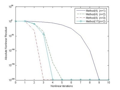
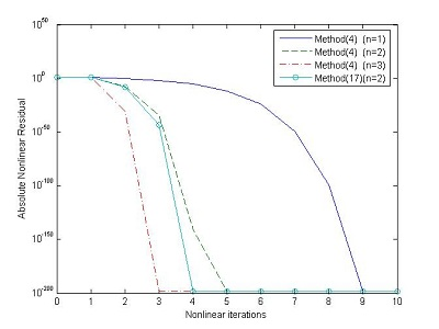
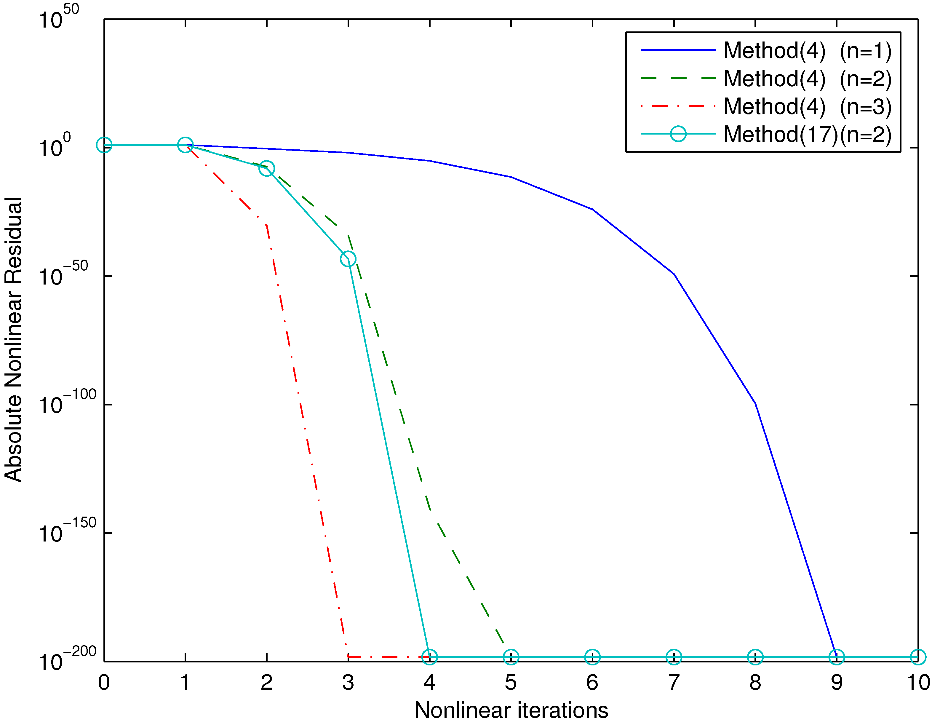
The iterative processes of the Equations (4) and (17) are given in Figure 1, where Equation (4) (n=1) is one-point method. The parameters of the Equations (4) and (17) are λ = λ 0 = 1 . 0 . The initial value is x 0 = - 1 . 3 . The stopping criterium is | f ( x ) | < 10 - 150 . We will call f ( x ) the nonlinear residual or residual. The Figure 1 is a semilog plot of residual history, the norm of the nonlinear residual against the iteration number.
Following test functions are used:
f 1 ( x ) = x e x 2 - sin 2 ( x ) + 3 cos ( x ) + 5 , a - 1 . 2076478271309189 , x 0 = - 1 . 3 .
f 2 ( x ) = x 5 + x 4 + 4 x 2 - 15 , a 1 . 3474280989683050 , x 0 = 1 . 6 .
Table 1. Numerical results for f 1 ( x ) by the methods without memory.
Methods | x 1 - a | | x 2 - a | | x 3 - a | ρ
Equation (4) n = 2 , λ = 0 . 5 0.32719E−40.57076E−180.52848E−734.0000005
Equation (4) n = 2 , λ = 1 0.58111E−40.71445E−170.16328E−683.9999938
K M 4 , β = 2 0.24269E−30.13078E−130.11033E−543.9999864
B R M 8 , h ( t ) = 1 + 2 t + 5 t 2 , γ = 1 0.40513E−60.32351E−480.53484E−3858.0000001
Equation (4) n = 3 , λ = 1 0.22673E−80.83510E−700.28282E−5618.0000000
Equation (4) n = 3 , λ = 1 . 5 0.18012E−90.75259E−830.69916E−6708.0000000
Table 2. Numerical results for f 2 ( x ) by the methods without memory.
Methods | x 1 - a | | x 2 - a | | x 3 - a | ρ
Equation (4) n = 2 , λ = - 1 . 5 0.29673E−20.37452E−100.94752E−424.0001713
Equation (4) n = 2 , λ = - 0 . 5 0.27276E−40.11867E−190.42516E−814.0000025
K M 4 , β = 0 . 5 0.37189E−20.32631E−90.19533E−373.9993916
B R M 8 , h ( t ) = 1 + 2 t + 5 t 2 , γ = 1 0.84179E−40.62964E−310.61512E−2488.0000456
Equation (4) n = 3 , λ = - 1 0.34838E−70.19030E−620.15080E−5048.0000000
Equation (4) n = 3 , λ = - 0 . 5 0.11873E−70.80149E−660.34562E−5318.0000000
Table 3. Numerical results for f 1 ( x ) by the methods with memory.
Methods | x 1 - a | | x 2 - a | | x 3 - a | ρ
Equation (42) - P D , γ 0 = - 0 . 01 0.10690E−20.10554E−120.24668E−584.5605896
Equation (43) - P D , γ 0 = - 0 . 01 0.10690E−20.58225E−140.18875E−674.7487424
Equation (14) - (17) , n = 2 , λ 0 = 0 . 5 0.32719E−40.42649E−190.26035E−874.5827899
Equation (15) - (17) , n = 2 , λ 0 = 0 . 5 0.32719E−40.47493E−200.16676E−964.8272294
Equation (14) - (17) , n = 2 , λ 0 = 1 0.58111E−40.25364E−180.61743E−844.5691828
Equation (15) - (17) , n = 2 , λ 0 = 1 0.58111E−40.28197E−190.69228E−934.8066915
Equation (14) - (17) , n = 3 , λ 0 = 1 0.22673E−80.14247E−760.38886E−6908.9963034
Equation (15) - (17) , n = 3 , λ 0 = 1 0.22673E−80.53419E−810.96778E−7779.5795515
Equation (16) - (17) , n = 3 , λ 0 = 1 0.22673E−80.45910E−830.96092E−8159.7957408
Equation (14) - (17) , n = 3 , λ 0 = 1 . 5 0.18012E−90.49194E−860.27126E−7759.0024260
Equation (15) - (17) , n = 3 , λ 0 = 1 . 5 0.18012E−90.13193E−910.20518E−8789.5794268
Equation (16) - (17) , n = 3 , λ 0 = 1 . 5 0.18012E−90.11706E−930.17692E−9189.7974669
Table 4. Numerical results for f 2 ( x ) by the methods with memory.
Methods | x 1 - a | | x 2 - a | | x 3 - a | ρ
Equation (42) - P D , γ 0 = - 0 . 01 0.14930E−10.54292E−80.20342E−374.5697804
Equation (43) - P D , γ 0 = - 0 . 01 0.14930E−10.32753E−90.16659E−454.7387964
Equation (14) - (17) , n = 2 , λ 0 = - 1 . 5 0.29673E−20.10381E−110.90169E−554.5538013
Equation (15) - (17) , n = 2 , λ 0 = - 1 . 5 0.29673E−20.13370E−130.29875E−674.7285160
Equation (14) - (17) , n = 2 , λ 0 = - 0 . 5 0.27276E−40.76276E−200.21310E−914.6005252
Equation (15) - (17) , n = 2 , λ 0 = - 0 . 5 0.27276E−40.62055E−210.70672E−1024.8635157
Equation (14) - (17) , n = 3 , λ 0 = - 1 0.34838E−70.12841E−670.15487E−6119.0002878
Equation (15) - (17) , n = 3 , λ 0 = - 1 0.34838E−70.34679E−730.10151E−7059.5835521
Equation (16) - (17) , n = 3 , λ 0 = - 1 0.34838E−70.41211E−750.11560E−7419.8127640
Equation (14) - (17) , n = 3 , λ 0 = - 0 . 5 0.11873E−70.35119E−730.13260E−6618.9795793
Equation (15) - (17) , n = 3 , λ 0 = - 0 . 5 0.11873E−70.43166E−770.67183E−7439.5883270
Equation (16) - (17) , n = 3 , λ 0 = - 0 . 5 0.11873E−70.45981E−830.29759E−8209.7754885
Figure 1. Iterative processes of different methods for the function f 1 ( x ) .
Algorithms 08 00786 g001

5. Conclusions

Figure 1 shows that the convergence speed of the multipoint iterative method is faster than the one-point iterative method. As shown in Table 1 and Table 2, the results obtained with our methods without memory are better than the other methods without memory. From the results displayed in Table 3 and Table 4, it can be concluded that the convergence of the tested multipoint Equation (17) with memory is remarkably fast. The R-order of convergence of the family Equation (17) with memory is increased by applying a self-accelerating parameter given by Equation (14)–Equation (16). In addition, above all, the increase of convergence order is obtained without any additional function evaluations, which indicates a very high computational efficiency of our methods with memory.

Acknowledgments

The project supported by the National Natural Science Foundation of China (Nos. 11371071 and 11201037), the PhD Start-up Fund of Liaoning Province of China ( Nos. 20141137 and 20141139), the Liaoning BaiQianWan Talents Program (No.2013921055) and the Educational Commission Foundation of Liaoning Province of China (Nos. L2014443,L2014444 and L2015012).

Author Contributions

Xiaofeng Wang and Yuping Qin conceived and designed the experiments; Weiyi Qian and Sheng Zhang analyzed the data; Xiaofeng Wang and Xiaodong Fan wrote the paper.

Conflicts of Interest

The authors declare no conflict of interest.

References

  1. Ortega, J.M.; Rheinbolt, W.C. Iterative Solution of Nonlinear Equations in Several Variables; Academic Press: New York, NY, USA, 1970. [Google Scholar]
  2. Wu, X. A new continuation Newton-like method and its deformation. Appl. Math. Comput. 2000, 112, 75–78. [Google Scholar] [CrossRef]
  3. Wang, X.; Zhang, T. A new family of Newton-type iterative methods with and without memory for solving nonlinear equations. Calcolo 2014, 51, 1–15. [Google Scholar] [CrossRef]
  4. Wang, X.; Liu, L. Modified Ostrowski’s method with eighth-order convergence and high efficiency index. Appl. Math. Lett. 2010, 23, 549–554. [Google Scholar] [CrossRef]
  5. Kou, J.; Wang, X.; Li, Y. Some eithth-order root-finding three-step methods. Commn. Nonli. Sci. Numer. Simulat. 2010, 15, 536–544. [Google Scholar] [CrossRef]
  6. Petković, M.S. Remarks on “on a general class of multipoint root-finding methods of high computational efficiency”. SIAM J. Numer. Anal. 2011, 49, 1317–1319. [Google Scholar] [CrossRef]
  7. Kung, H.T.; Traub, J.F. Optimal order of one-point and multipoint iterations. J. Appl. Comput. Math. 1973, 10, 643–651. [Google Scholar] [CrossRef]
  8. Alefeld, G.; Herzberger, J. Introduction to Interval Computation; Academic Press: New York, NY, USA, 1983. [Google Scholar]
  9. King, R.F. A family of fourth order methods for nonlinear equations. SIAM J. Numer. Anal. 1973, 10, 876–879. [Google Scholar] [CrossRef]
  10. Bi, W.; Wu, Q.; Ren, H. A new family of eighth-order iterative methods for solving nonlinear equations. Appl. Math. Comput. 2009, 214, 236–245. [Google Scholar] [CrossRef]
  11. Petković, M.S.; Ilić, S.; Džuni, J. Derivative free two-point methods with and without memory for solving nonlinear equations. Appl. Math. Comput. 2010, 217, 1887–1895. [Google Scholar] [CrossRef]
  12. Thukral, R.; Petković, M.S. A family of three-point methods of optimal order for solving nonlinear equations. J. Comp. Appl. Math. 2010, 223, 2278–2284. [Google Scholar] [CrossRef]
  13. Wang, X.; Zhang, T. A family of Steffensen type methods with seventh-order convergence. Numer. Algor. 2013, 62, 429–444. [Google Scholar] [CrossRef]
  14. Wang, X.; Džunić, J.; Zhang, T. On an efficient family of derivative free three-point methods for solving nonlinear equations. Appl. Math. Comput. 2012, 219, 1749–1760. [Google Scholar] [CrossRef]
  15. Soleymani, F.; Sharifi, M.; Mousavi, B.S. An inprovement of Ostrowski’s and King’s techniques with optimal convergence order eight. J. Optim. Theory. Appl. 2012, 153, 225–236. [Google Scholar] [CrossRef]
  16. Yun, B.I. A non-iterative method for solving non-linear equations. Appl. Math. Comput. 2008, 198, 691–699. [Google Scholar] [CrossRef]
  17. Sharma, J.R.; Sharma, R. A new family of modified Ostrowski’s methods with accelerated eighth order convergence. Numer. Algor. 2010, 54, 445–458. [Google Scholar] [CrossRef]
  18. Cordero, A.; Ezquerro, J.A.; Hernánde-Verón, M.A.; Torregrosa, J.R. On the local convergence of a fifth-order iterative method in Banach spaces. Appl. Math. Comput. 2015, 215, 396–403. [Google Scholar] [CrossRef]
  19. Grau-Sánchez, M.; Noguera, M.; Gutiérrez, J.M. On some computational orders of convergence. Appl. Math. Lett. 2010, 23, 472–478. [Google Scholar] [CrossRef]

