A Data Analytic Algorithm for Managing, Querying, and Processing Uncertain Big Data in Cloud Environments

Abstract

Big data are everywhere as high volumes of varieties of valuable precise and uncertain data can be easily collected or generated at high velocity in various real-life applications. Embedded in these big data are rich sets of useful information and knowledge. To mine these big data and to discover useful information and knowledge, we present a data analytic algorithm in this article. Our algorithm manages, queries, and processes uncertain big data in cloud environments. More specifically, it manages transactions of uncertain big data, allows users to query these big data by specifying constraints expressing their interests, and processes the user-specified constraints to discover useful information and knowledge from the uncertain big data. As each item in every transaction in these uncertain big data is associated with an existential probability value expressing the likelihood of that item to be present in a particular transaction, computation could be intensive. Our algorithm uses the MapReduce model on a cloud environment for effective data analytics on these uncertain big data. Experimental results show the effectiveness of our data analytic algorithm for managing, querying, and processing uncertain big data in cloud environments.

1. Introduction

Big data [1,2,3] are everywhere. They are high-veracity, high-velocity, high-value, and/or high-variety data with volumes beyond the ability of commonly-used software to manage, query, and process within a tolerable elapsed time. These high volumes of valuable data can be easily collected or generated at a high velocity from different data sources (which may lead to different data formats) in various real-life applications such as bioinformatics, graph management, sensor and stream systems, smart worlds, social networks, as well as the Web [4,5,6,7,8]. Characteristics of these big data can be described by the following “5 Vs”:

• Veracity, which focuses on the quality of data (e.g., uncertainty, messiness, or trustworthiness of data);
• Velocity, which focuses on the speed at which data are collected or generated;
• Value, which focuses on the usefulness of data;
• Variety, which focuses on differences in types, contents or formats of data; and
• Volume, which focuses on the quantity of data.

Embedded in the big data (e.g., biological data, medical images, streams of advertisements, surveillance videos, business transactions, financial charts, social media data, web logs, texts and documents) are rich sets of useful information and knowledge. Due to the “5 Vs” characteristics of big data, new forms of algorithm are needed for managing, querying, and processing these big data so as to enable enhanced decision making, insight, process optimization, data mining and knowledge discovery. This drives and motivates research and practices in data science, which aims to develop systematic or quantitative data analytic algorithm to analyze (e.g., inspect, clean, transform, and model) and mine big data.

Big data analytics [9,10,11,12] incorporates various techniques from a broad range of fields, which include cloud computing, data mining, machine learning, mathematics, and statistics. Data mining aims to extract implicit, previously unknown, and potentially useful information from data. With “5 Vs” characteristics of big data, it is natural to handle the data in a cloud computing environment as a cloud environment represents a “natural” context for big data by providing high performance, reliability, availability, transparency, abstraction, and/or virtualization. Various approaches—ranging from mathematical models to approximation models, from resource-constrained paradigms to memory-bounded methods—can be applied in cloud computing environments. Over the past few years, algorithms for handling big data according to a “systematic” view of the problem (e.g., MapReduce algorithms) are gaining momentum.

MapReduce [13] is a high-level programming model for handling high volumes of big data by using parallel and distributed computing [14,15,16] on clouds [17,18,19], which consist of a master node and multiple worker nodes. As implied by its name, MapReduce involves two key functions: “map” and “reduce” functions commonly used in functional programming languages such as LISP for list processing:

• The mapper applies a mapping function to each value in the list of values and returns the resulting list;
• The reducer applies a reducing function to combine all the values in the list of values and returns the combined result.

An advantage of using the MapReduce model is that users only need to focus on (and specify) these “map” and “reduce” functions—without worrying about implementation details for the following:

• handling machine failures,
• managing inter-machine communication,
• partitioning the input data, or
• scheduling and executing the program across multiple machines.

Several algorithms have been proposed over the past few years to use the MapReduce model—which mines the search space with parallel, distributed, or cloud computing—for big data analytics tasks like classification [20] and clustering [21]. In contrast, we focus on another big data analytics task—namely, association rule mining [22], which discovers interesting knowledge in the form of association rules $A\Rightarrow C$ revealing associative relationships between (i) shopper market baskets A and C of frequently purchased merchandise items or (ii) collections A and C of frequently co-located events.

By applying association rule mining to valuable big market basket data, data scientists can help shop owners/managers find interesting or popular patterns that reveal customer purchase behaviour. The research problem of association rule mining usually consists of two key steps:

• Mining of frequent patterns [23], and
• Formation of association rules (by using the mined frequent patterns as antecedents and consequences of the rules).

Since the introduction of the frequent pattern mining problem [22], numerous studies [24,25,26] have been conducted (e.g., mining frequent patterns from traditional databases of shopper market basket transactions). With these traditional databases of precise data, users definitely know whether an item is present in (or is absent from) a transaction. In contrast, data in many real-life applications are riddled with uncertainty [27,28,29,30,31]. It is partially due to inherent measurement inaccuracies, sampling and duration errors, network latencies, or intentional blurring of data to preserve anonymity. As such, users are usually uncertain about the presence or absence of items. As a concrete example, a physician may highly suspect (but cannot guarantee) that a coughing patient suffers from the Middle East respiratory syndrome (MERS). The uncertainty of such suspicion can be expressed in terms of existential probability (e.g., a 60% likelihood of suffering from the MERS). With this notion, each item in a transaction $t_j$ in databases containing precise data can be viewed as an item with a 100% likelihood of being present in $t_j$. To find frequent patterns from uncertain data, several uncertain data mining algorithms (e.g., UF-growth [32], tube-growth [33], and BLIMP-growth [34] algorithms) have been proposed.

For many real-life applications, users look for all frequent patterns. However, for some other real-life applications, users may have some particular phenomena in mind on which to focus the mining (e.g., a physician may want to find only those patients who are suffering from MERS). To avoid waiting for a long period of time for numerous patterns out of which only a tiny fraction may be interesting to the users, constrained pattern mining [35]—which aims to find those patterns that satisfy the user-specified constraints—is in demand. For example, we previously [36] exploited a special class of constraints called SAM constraints. Such exploitation helps reduce the search space when mining patterns satisfying user-specified SAM constraints. However, many commonly used constraints (e.g., sum(X.Expenses) < 300 CHF, which finds every combination X of items with a total cost less than 300 CHF) do not belong to the class of SAM constraints. In the current article, we explore another class of constraints, called anti-monotone (AM) constraints, to which commonly used constraints belong. We explore two sub-classes of anti-monotone constraints: (i) the frequency constraint; and (ii) non-frequency AM constraints.

In this article, our key contribution is our data analytic algorithm called MrCloud—which uses the MapReduce model in cloud environments for managing, querying, and processing uncertain big data. More specifically, MrCloud manages transactions of uncertain big data, allows users to query these big data by specifying anti-monotone constraints expressing their interests, and processes the user-specified constraints to discover useful information and knowledge in the form of frequent patterns from the uncertain big data. So, MrCloud can be considered as a non-trivial integration of (i) frequent pattern mining; (ii) big data mining; (iii) constrained mining; and (iv) uncertain data mining.

The remainder of this article is organized as follows. The next section presents background and related works. In Section 3, we propose our data analytic algorithm for mining patterns satisfying AM constraints from uncertain big data using MapReduce. Evaluation results and conclusions are given in Section 4 and Section 5, respectively.

2. Background and Related Works

In this section, we present some background information and related works on extensions of frequent pattern mining, namely (Section 2.1) big data mining with the MapReduce model, (Section 2.2) constrained mining, and (Section 2.3) uncertain data mining.

2.1. Big Data Mining with the MapReduce Model

MapReduce [13] is a high-level programming model for processing vast amounts of data. It usually uses parallel and distributed computing on clouds of nodes (i.e., computers). As implied by its name, MapReduce involves two key functions: “map” and “reduce”.

First, the input data are read, divided into several partitions (sub-problems), and assigned to different processors. Each processor executes the map function on each partition (sub-problem). The map function takes a pair of $\langle key,value\rangle$ and returns a list of $\langle key,value\rangle$ pairs as an intermediate result:

$$\mathrm{map}:\langle ke{y}_1,valu{e}_1\rangle \mapsto \mathrm{list}\mathrm{of}\langle ke{y}_2,valu{e}_2\rangle$$

where (i) $ke{y}_1$ & $ke{y}_2$ are keys in the same or different domains; and (ii) $valu{e}_1$ & $valu{e}_2$ are the corresponding values in some domains.

Afterwards, the pairs returned by the map function are shuffled and sorted. Each processor then executes the reduce function on (i) a single key from this intermediate result together with (ii) the list of all values that appear with this key in the intermediate result. The reduce function “reduces”—by combining, aggregating, summarizing, filtering, or transforming—the list of values associated with a given key (for all k keys) and returns a single (aggregated or summarized) value:

$$\mathrm{reduce}:\langle ke{y}_2,\mathrm{list}\mathrm{of}valu{e}_2\rangle \mapsto valu{e}_3$$

where (i) $ke{y}_2$ is a key in some domains; and (ii) $valu{e}_2$ & $valu{e}_3$ are the corresponding values in some domains. Examples of MapReduce applications include the construction of an inverted index as well as the word counting of a document for data processing [13].

To mine frequent patterns from precise data using the MapReduce model, three Apriori-based algorithms called SPC, FPC and DPC [37] were proposed. Among them, SPC uses single-pass counting to find frequent patterns of cardinality k at the k-th pass (i.e., the k-th database scan) for $k\ge 1$. FPC uses fixed-passes combined-counting to find all patterns of cardinalities k, $(k+1)$, ..., $(k+m)$ in the same pass or database scan. On the one hand, this fixed-passes technique fixes the number of required passes from $k_{max}$ (where $k_{max}$ is the maximum cardinality of all frequent patterns that can be mined from the precise data) to a user-specified constant. On the other hand, due to combined-counting, the number of generated candidates is higher than that of SPC. In contrast, DPC uses dynamic-passes combined-counting, which takes the benefits of both SPC and FPC by taking into account the workloads of nodes when mining frequent patterns with MapReduce. In addition, a parallel randomized algorithm called PARMA [38] was proposed for mining approximations to the top-k frequent patterns and association rules from precise data by using MapReduce.

As a preview, our MrCloud algorithm also uses MapReduce. However, unlike SPC, FPC or DPC [37] (which use the Apriori-based approach to mine frequent patterns from precise data), our MrCloud uses a tree-based approach to mine frequent patterns from uncertain data—which deals with a much larger search space than that for mining precise data due to the presence of the existential probability values. Moreover, unlike PARMA (which mines all of the approximately frequent patterns from precise data), our data analytic algorithm mines some—specifically, those interesting patterns that satisfy the user-specified constraints—of the truly frequent patterns from uncertain data.

2.2. Constrained Mining

Allowing users to specify their interest via the use of constraints [35,39,40] helps guide the data mining process so that only those sets of frequently co-occurring items satisfying the user-specified constraints can be found, which in turn avoids unnecessary computation for mining those uninteresting frequent patterns. These user-specified constraints can be imposed on items, events or objects in various domains, including shopper market baskets, meteorological records, and event planning calendars. In general, these constraints can be categorized into several overlapping classes according to the properties that they possess. In this article, we examine one class of constraints called anti-monotone (AM) constraints, which possess the properties of anti-monotonicity. This class of constraints can be further subdivided into the following two sub-classes:

• Frequency constraints include the following:

  • $C_1\equiv$ sup(X) ≥ minsup expresses the user interest in finding frequent patterns from precise data, i.e., every pattern X with actual support (or frequency) meeting or exceeding the user-specified minimum support threshold minsup; and $C_2\equiv$ expSup(X) ≥ minsup expresses the user interest in finding frequent patterns from uncertain data, i.e., every pattern X with expected support meeting or exceeding the user-specified minimum support threshold minsup.
• Non-frequency AM constraints, with examples include the following:

  • $C_3\equiv$ min(X.RewardPoints) ≥ 2000 expresses the user interest in finding every pattern X such that the minimum reward points earned by travellers among all airports visited are at least 2000;
  • $C_4\equiv$ max(X.Rainfall) ≤ 10 mm says that the maximum rainfall among all meteorological records in X is at most 10 mm (i.e., “relatively dry”);
  • $C_5\equiv$ X.Location = Europe expresses the user interest in finding every pattern X such that all places in X are located in Europe;
  • $C_6\equiv$ X.Weight ≤ 23 kg says that the weight of each object in X is at most 23 kg (e.g., no heavy checked baggage for a trip); and
  • $C_7\equiv$ sum(X.Expenses) < 300 CHF says that the total expenses on all items in X is less than 300 CHF.

Note that a constraint C is anti-monotone [40] if and only if all subsets of a pattern satisfying C also satisfy C. Equivalently, a constraint C is anti-monotone (AM) if and only if all supersets of a pattern violating C also violate C. A pattern X is valid in a database if such a pattern also satisfies the user-specified constraints. Given (i) a database; (ii) user-specified minsup; and (iii) user-specified AM constraints, the research problem of constrained pattern mining from uncertain data is to discover from the database a complete set of patterns satisfying the user-specified AM constraints (i.e., valid patterns).

2.3. Uncertain Data Mining

Let (i) Item be a set of m domain items and (ii) $X=\{x_1,x_2,\cdots ,x_k\}$ be a k-itemset (i.e., a pattern consisting of k items), where $X\subseteq$ Item and $1\le k\le m$. Then, a transactional database is the set of n transactions, where each transaction $t_j\subseteq$ Item (for $1\le j\le n$). The projected database of X is the set of all transactions containing X. Each item $x_i$ in a transaction $t_j=\{x_1,x_2,\cdots ,x_h\}$ in an uncertain database is associated with an existential probability $P(x_i,t_j)$, which represents the likelihood of the presence of $x_i$ in $t_j$ [41], with value

$$0<P(x_i,t_j)\le 1$$

The existential probability $P(X,t_j)$ of a pattern X in $t_j$ is then the product of the corresponding existential probabilities of every item $x_i$ within X when these items are independent [41,42]:

$$P(X,t_j)=\prod _{x_i\in X}P(x_i,t_j)$$

Finally, the expected support expSup(X) of X is the sum of $P(X,t_j)$ over all n transactions in the database:

$$\mathit{expSup}\left(X\right)=\sum _{j=1}^{n}P(X,t_j)=\sum _{j=1}^n\left(\prod _{x_i\in X}P(x_i,t_j)\right)$$

(1)

With this notion of expected support, existing tree-based algorithms—such as UF-growth [32], tube-growth [33] and BLIMP-growth [34]—mine frequent patterns from uncertain data by first scanning the uncertain database once to compute the expected support of all domain items (i.e., singleton patterns). Infrequent items are pruned as their extensions/supersets are guaranteed to be infrequent. The algorithms then scan the database a second time to insert all transactions (with only frequent items) into a tree (e.g., UF-tree [32], TPC-tree [33], or BLIMP-tree [34]). Each node in the tree captures (i) an item x; (ii) its existential probability $P(x,t_j)$; and (iii) its occurrence count. At each step during the mining process, the frequent patterns are expanded recursively.

A pattern X is frequent in an uncertain database if $\mathit{expSup}\left(X\right)\ge$ minsup. Given a database and minsup, the research problem of frequent pattern mining from uncertain data is to discover from the database a complete set of frequent patterns having expected support ≥ minsup.

3. MrCloud: Our Data Analytic Algorithm

Given (i) uncertain big data; (ii) user-specified minsup; (iii) a user-specified constraint C (e.g., an AM constraint), the research problem of constrained frequent pattern mining from uncertain big data is to discover from big data a complete set of patterns having expected support ≥ minsup and satisfying C (i.e., valid frequent patterns). In this section, we present our data analytic algorithm—called MrCloud—that uses MapReduce for managing, querying, and processing uncertain big data in cloud environments. Specifically, our algorithm manages transactions of uncertain big data, allows users to query these big data by specifying constraints expressing their interests, and processes the user-specified constraints to discover useful information and knowledge from the uncertain big data.

3.1. Managing Uncertain Big Data

To manage uncertain big data, our MrCloud algorithm keeps track of both (i) the transactions of uncertain data; and (ii) an auxiliary file capturing information about domain items in uncertain data. Here, items in each transaction of uncertain data are associated with existential probability values expressing the likelihood of these items in the transaction in the form of a set of every item $x_i$ with its existential probability value $P(x_i,t_j)$:

$$\{x_i:P(x_i,t_j)\}$$

See Table 1 for an illustrative sample capturing transactions of uncertain data collected about the airports visited by travellers. Also see Table 2 for the auxiliary information about reward points that can be earned by travellers visiting those airports. For instance, $t_1$ captures the uncertain data that a traveller may have visited six airports (namely, AMS, BCN, CPH, DEL, EDI and FRA). Among them, it is 100% sure that he has visited BCN and EDI (where he earned 3000 and 2000 points, respectively). There is a 90% chance that he has visited AMS or DEL (where he would earn 2400 and 3200 points, respectively), 50% chance that he has visited CPH (where he would earn 2600 points), and only 20% chance that he has visited FRA (where he would earn 2200 points).

Table 1. An illustrative sample set of uncertain big data.

TID	Content
$t_1$	{AMS: 0.9, BCN: 1.0, CPH: 0.5, DEL: 0.9, EDI: 1.0, FRA: 0.2}
$t_2$	{AMS: 0.8, BCN: 0.8, CPH: 1.0, EDI: 0.2, FRA: 0.2, IST: 0.6}
$t_3$	{AMS: 0.4, FRA: 0.2, GUM: 1.0, HEL: 0.5}

Table 1. An illustrative sample set of uncertain big data.

TID	Content
$t_1$	{AMS: 0.9, BCN: 1.0, CPH: 0.5, DEL: 0.9, EDI: 1.0, FRA: 0.2}
$t_2$	{AMS: 0.8, BCN: 0.8, CPH: 1.0, EDI: 0.2, FRA: 0.2, IST: 0.6}
$t_3$	{AMS: 0.4, FRA: 0.2, GUM: 1.0, HEL: 0.5}

Table 2. Auxiliary information for the uncertain big data in Table 1.

IATA Code	Airport	Reward Points
AMS	Amsterdam	2400
BCN	Barcelona	3000
CPH	Copenhagen	2600
DEL	Delhi	3200
EDI	Edinburgh	2000
FRA	Frankfurt	2200
GUM	Guam	1800
HEL	Helsinki	2800
IST	Istanbul	1600

Table 2. Auxiliary information for the uncertain big data in Table 1.

IATA Code	Airport	Reward Points
AMS	Amsterdam	2400
BCN	Barcelona	3000
CPH	Copenhagen	2600
DEL	Delhi	3200
EDI	Edinburgh	2000
FRA	Frankfurt	2200
GUM	Guam	1800
HEL	Helsinki	2800
IST	Istanbul	1600

3.2. Querying Uncertain Big Data

Once our MrCloud algorithm managed uncertain big data, it allows users to query the data. Users can express their interests by selecting one of SQL-style constraints in the form of (i) “X.attribute θ constant”; (ii) “agg(X.attribute) θ constant”; and (iii) their logical combinations via the conjunction operator “AND” (∧) or the disjunction operator “OR” (∨), where (i) agg is an aggregate function including max, min, sum, and (ii) θ is a comparison operator including $>,\ge ,=,\le ,<$. Examples are not confined to the aforementioned (i) frequency constraints $C_1$ & $C_2$ or (ii) non-frequency AM constraints $C_3$–$C_7$, users can also specify AM constraints involving more than one aggregate function. The following is an example:

• $C_8\equiv$ difference(X.Temperature) = max(X.Temperature) − min(X.Temperature) ≤ 10 °C says that the difference between the maximum and minimum temperatures in X is at most 10 °C (which involves the difference between two aggregate functions maximum and minimum).

Moreover, users can also specify constraints involving more than one AM constraint. Examples include the following:

• $C_9\equiv$ [min(X.Temperature) ≥ 20 °C] ∧ [max(X.Temperature) ≤ 30 °C] expresses the user interest in finding every pattern X with temperature between 20 °C to 30 °C inclusive (which involves a logical conjunction “AND” of two AM constraints);
• $C_{10}\equiv$ [min(X.RewardPoints) ≥ 2000] ∧ [X.Location = Europe] expresses the user interest in finding every pattern X such that the minimum reward points earned by travellers among all European airports visited are at least 2000 (which again involves a logical conjunction “AND” of two AM constraints); and
• $C_{11}\equiv$ [min(X.Temperature) ≥ 20 °C] ∨ [max(X.Rainfall) ≤ 10 mm] expresses the user interest in finding all meteorological records matching “warm” or “relatively dry” patterns (which involves a logical conjunction “OR” of two AM constraints).

Last but not least, users can also specify constraints that are not AM (e.g., $C_{12}\equiv$ avg(X.Temperature) ≥ 25 °C expressing the user interest in finding every pattern X with average temperature at least 25 °C). Since the users specify their constraints by selecting one of the SQL-style constraints, MrCloud can easily determine whether the user-specified constraints are AM or not. Table 3 shows examples of the classification.

Table 3. Classification of some AM and non-AM constraints.

Classification	Constraints
AM	X.attribute θ constant, where $\theta \in \{>,\ge =,\le ,<\}$
	max(X.attribute) θ constant, where $\theta \in \{=,\le ,<\}$
	min(X.attribute) θ constant, where $\theta \in \{>,\ge ,=\}$
	sum(X.attribute) θ constant, where $\theta \in \{\le ,<\}$
	$C_1\wedge C_2$, where $C_1$ and $C_2$ are AM constraints
	$C_1\vee C_2$, where $C_1$ and $C_2$ are AM constraints
non-AM	max(X.attribute) θ constant, where $\theta \in \{>,\ge \}$
	min(X.attribute) θ constant, where $\theta \in \{\le ,<\}$
	sum(X.attribute) θ constant, where $\theta \in \{>,\ge \}$
	avg(X.attribute) θ constant, where $\theta \in \{>,\ge ,=,\le ,<\}$

Table 3. Classification of some AM and non-AM constraints.

Classification	Constraints
AM	X.attribute θ constant, where $\theta \in \{>,\ge =,\le ,<\}$
	max(X.attribute) θ constant, where $\theta \in \{=,\le ,<\}$
	min(X.attribute) θ constant, where $\theta \in \{>,\ge ,=\}$
	sum(X.attribute) θ constant, where $\theta \in \{\le ,<\}$
	$C_1\wedge C_2$, where $C_1$ and $C_2$ are AM constraints
	$C_1\vee C_2$, where $C_1$ and $C_2$ are AM constraints
non-AM	max(X.attribute) θ constant, where $\theta \in \{>,\ge \}$
	min(X.attribute) θ constant, where $\theta \in \{\le ,<\}$
	sum(X.attribute) θ constant, where $\theta \in \{>,\ge \}$
	avg(X.attribute) θ constant, where $\theta \in \{>,\ge ,=,\le ,<\}$

3.3. Processing Uncertain Big Data

Once the users queried uncertain big data by specifying their constraints that express their interest, our MrCloud algorithm processes these user-specified queries to find frequent patterns that satisfy these user-specified constraints. Given (i) an implicit frequency constraint $C_2\equiv$ expSup(X) ≥ minsup; and (ii) an explicit user-specified constraints, MrCloud explores the anti-monotonicity of these constraints in pruning the search space. More specifically, the implicit frequency constraint satisfies the anti-monotonicity:

• If a pattern X is frequent (i.e., expSup(X) ≥ minsup), then all subsets of X are guaranteed to satisfy the AM constraints because expSup($X^{\prime }$) ≥ expSup(X) ≥ minsup for every subset $X^{\prime }\subseteq X$.
• If a pattern Y is infrequent (i.e., expSup(Y) < minsup), then all supersets of Y are guaranteed to be infrequent because expSup($Y^{\prime }$) < expSup(Y) < minsup for every superset $Y^{\prime }\supseteq Y$. Thus, every superset $Y^{\prime }$ of Y can be pruned.

However, if a pattern X is frequent, then some supersets of X may be frequent while some other may not be frequent. Thus, frequency checking is needed to be applied to every superset of X. Similarly, if the user-specified constraint satisfies the anti-monotonicity, then we can prune the search space due to the following:

• If a pattern X satisfies AM constraints, then all subsets of X are guaranteed to satisfy the AM constraints.
• If a pattern Y does not satisfy AM constraints, then all supersets of Y are guaranteed not to satisfy the AM constraints and thus can be pruned.

However, if a pattern X satisfies AM constraints, then some supersets of X may satisfy the AM constraints while some other may not satisfy the AM constraints. Thus, constraint checking is needed to be applied to every superset of X. These observations about anti-monotone constraints hold not only for constraints involving one AM constraint but also constraints involving multiple AM constraints due to the following.

Theorem 1. 

If constraints $C_a$ and $C_b$ are anti-monotone, then the constraint ($C_a\wedge C_b$) is also anti-monotone.

Proof. 

For anti-monotone constraints $C_a$ and $C_b$, if a pattern X satisfies $C_a$ and $C_b$, then all subsets of X are guaranteed to satisfy $C_a$ and satisfy $C_b$. In other words, all subsets of X are guaranteed to satisfy ($C_a\wedge C_b$). Conversely, if a pattern Y does not satisfy $C_a$ and does not satisfy $C_b$, then all supersets of Y are guaranteed not to satisfy $C_a$ and not to satisfy $C_b$. In other words, all supersets of Y are guaranteed not to satisfy ($C_a\wedge C_b$). Thus, ($C_a\wedge C_b$) is also anti-monotone. ☐

Theorem 2. 

If constraints $C_a$ or $C_b$ are anti-monotone, then the constraint ($C_a\vee C_b$) is also anti-monotone.

Proof. 

For anti-monotone constraints $C_a$ or $C_b$, if a pattern X satisfies $C_a$ and $C_b$, then all subsets of X are guaranteed to satisfy $C_a$ or satisfy $C_b$. In other words, all subsets of X are guaranteed to satisfy ($C_a\vee C_b$). Conversely, if a pattern Y does not satisfy $C_a$ or does not satisfy $C_b$, then all supersets of Y are guaranteed not to satisfy $C_a$ or not to satisfy $C_b$. In other words, all supersets of Y are guaranteed not to satisfy ($C_a\vee C_b$). Thus, ($C_a\vee C_b$) is also anti-monotone. ☐

On the other hand, if the explicit user-specified constraints do not satisfy anti-monotonicity, our MrCloud first discovers all frequent patterns and then verifies the validity of each of these discovered patterns to see if it satisfies the user-specified constraints at a post-processing step.

To process uncertain big data, our MrCloud algorithm first reads and divides the uncertain big data into several partitions and assigns them to different processors. The map function (denoted as ${\mathrm{map}}_1$) receives 〈transaction ID, content of that transaction〉 as input. To facilitate time-efficient and space-efficient constrained frequent pattern mining, MrCloud pushes the user-specified non-frequency AM constraints $C_{\mathit{AM}}$ early in the mining process by pushing them into the ${\mathrm{map}}_1$ function. So, for every transaction $t_j$, the ${\mathrm{map}}_1$ function performs constraint checking for $C_{\mathit{AM}}$ and emits an $\langle x,P(x,t_j)\rangle$ pair for each occurrence of valid item $x\in t_j$ (i.e., those domain items satisfying the non-frequency AM constraints):

$${\mathrm{map}}_1:\langle \mathrm{ID}\mathrm{of}\mathrm{transaction}{t}_j,\mathrm{content}\mathrm{of}{t}_j\rangle \mapsto \mathrm{list}\mathrm{of}\langle \mathrm{valid}x,P(x,t_j)\rangle$$

(2)

In other words, by specifying the following, the ${\mathrm{map}}_1$ function produces a list of 〈valid $x,P(x,t_j)\rangle$ pairs with many different valid x and $P(x,t_j)$ for the keys and values:

        for each tj ∈  partition of the uncertain big data do
           for each item x ∈ tj and {x}  satisfies CAM do
              emit 〈x, P(x, tj)〉.
		

Afterwards, these 〈valid $x,P(x,t_j)\rangle$ pairs are shuffled and sorted. Each processor then executes the reduce function (denoted as ${\mathrm{reduce}}_1$) on the shuffled and sorted pairs to obtain the expected support of x. Recall that each item in the uncertain big data is associated with an existential probability value. The ${\mathrm{reduce}}_1$ function computes the expected support of all domain items (i.e., singleton patterns) by using MapReduce with Equation (1), which can be simplified to become the following when computing singleton patterns:

$$\mathit{expSup}\left(\left\{x\right\}\right)=\sum _{j=1}^{n}P(x,t_j)$$

(3)

where $P(x,t_j)$ is an existential probability of item x in transaction $t_j$. In other words, the ${\mathrm{reduce}}_1$ function sums all existential probabilities of x for each valid x to compute its expected support:

$${\mathrm{reduce}}_1:\langle \mathrm{valid}x,\mathrm{list}\mathrm{of}P(x,t_j)\rangle \mapsto \mathrm{list}\mathrm{of}\langle \mathrm{valid}\mathrm{frequent}\left\{x\right\},\mathit{expSup}\left(\right\{x\left\}\right)\rangle$$

(4)

More specifically, the ${\mathrm{reduce}}_1$ function finds those items satisfying the frequency constraints by specifying the following:

           for each x ∈ 〈valid x,list of P(x,tj)〉 do
              set expSup({x}) = 0;
              for each P(x,tj) ∈ list of P(x,tj) do
                 expSup({x}) = expSup({x}) + P(x,tj);
              if expSup({x}) ≥ minsup then
                 emit 〈{x},expSup({x})〉.
		

For the explicit user-specified non-frequency non-AM constraints $C_{\mathit{nonAM}}$, our MrCloud verifies the validity of each discovered frequent $\left\{x\right\}$ returned by the ${\mathrm{reduce}}_1$ function to see if it satisfies the user-specified constraints. Consequently, we obtain all valid frequent singletons (i.e., domain items that satisfy the user-specified constraints) and their associated existential support values.

MrCloud then proceeds to the next step, which is computationally intensive, by rereading each transaction in the uncertain big data to form an $\left\{x\right\}$-projected database (i.e., a collection of all prefixes of transactions ending with x) for each valid frequent singleton $\left\{x\right\}$ returned by the ${\mathrm{reduce}}_1$ function. This second map function (denoted as ${\mathrm{map}}_2$)

$${\mathrm{map}}_2:\langle \mathrm{ID}\mathrm{of}\mathrm{transaction}{t}_j,\mathrm{content}\mathrm{of}{t}_j\rangle \mapsto \mathrm{list}\mathrm{of}\langle \mathrm{valid}\mathrm{frequent}\left\{x\right\},\mathrm{part}\mathrm{of}{t}_j\mathrm{with}x\rangle$$

(5)

can be specified as follows:

           for each tj ∈ partition of the uncertain big data do
              for each {x} ∈ 〈{x}, expSup({x})〉 do
                 if prefix of tj ending with x contains items besides x then
                    emit 〈{x}, prefix of tj ending with x〉.
		

The worker node corresponding to each partition helps to form an $\left\{x\right\}$-projected database for every valid frequent item x in the transactions assigned to that partition. The $\left\{x\right\}$-projected database consists of prefixes of relevant transactions (from the uncertain big data) that end with x. More precisely, the worker node outputs $\langle \left\{x\right\}$, portion of $t_j$ for forming the $\left\{x\right\}$-projected database〉 pairs.

Then, the reduce function

$${\mathrm{reduce}}_2:\langle \mathrm{valid}\mathrm{frequent}\left\{x\right\},\left\{x\right\}-\mathrm{projected}\mathrm{database}\rangle \mapsto \mathrm{list}\mathrm{of}\langle \mathrm{valid}\mathrm{frequent}X,\mathit{expSup}\left(X\right)\rangle$$

(6)

shuffles and sorts these pairs of $\left\{x\right\}$-projected databases, from which valid frequent non-singleton patterns can be found and their expected support values can be computed. As any non-singleton patterns containing valid singleton items are not guaranteed to be valid, additional constraint check on AM constraints $C_{\mathit{AM}}$ is required when forming the projected database in mining valid frequent patterns. So, the worker node corresponding to each projected database then builds appropriate trees (e.g., UF-tree, TPC-tree, or BLIMP-tree)—based on the projected databases assigned to the worker node—to mine every valid frequent non-singleton pattern X (with cardinality k, where $k\ge 2$). The worker node also outputs $\langle X,\mathit{expSup}\left(X\right)\rangle$, i.e., every valid frequent non-singleton pattern with its expected support:

	for each x ∈ {x}-projected database do
           build a tree for {x}-projected database to find X;
           if X satisfies CAM and expSup(X) ≥ minsup then
              emit 〈X, expSup(X)〉.
		 

Again, for the explicit user-specified non-frequency non-AM constraints $C_{\mathit{nonAM}}$, our MrCloud verifies the validity of each discovered frequent X returned by the ${\mathrm{reduce}}_2$ function to see if it satisfies the user-specified constraints.

Example 1. 

Let us consider an illustrative sample set of an uncertain big database (as shown in Table 1) and its auxiliary information (as shown in Table 2) with (i) the user-specified minsup=0.9; and (ii) a user-specified constraint $C_{10}\equiv$ [min(X.RewardPoints) ≥ 2000] ∧ [X.Location = Europe] (which expresses the user interest in finding every pattern X such that the minimum reward points earned by travellers among all European airports visited are at least 2000). Based on the auxiliary information, we learn that airports AMS, BCN, CPH, EDI, FRA and HEL (but not DEL, GUM or IST) satisfy $C_{10}$. More specifically, (i) both DEL and GUM are not in Europe; and (ii) travellers visiting either GUM or IST would not be able to earn at least 2000 reward points.

Then, for the first transaction $t_1$, the ${\mathit{map}}_1$ function outputs only 〈AMS, 0.9〉, 〈BCN, 1.0〉, 〈CPH, 0.5〉, 〈EDI, 1.0〉 and 〈FRA, 0.2〉. Similarly, for the second transaction $t_2$, the ${\mathit{map}}_1$ function outputs 〈AMS, 0.8〉, 〈BCN, 0.8〉, 〈CPH, 1.0〉, 〈EDI, 0.2〉, and 〈FRA, 0.2〉. For the third transaction $t_3$, the ${\mathit{map}}_1$ function outputs only 〈AMS, 0.4〉, 〈FRA, 0.2〉 and 〈HEL, 0.5〉. These output pairs are then shuffled and sorted.

Note that the ${\mathit{map}}_1$ function does not output 〈DEL, 0.9〉 for $t_1$ because {DEL} does not satisfy $C_{10}$. Moreover, it also does not output 〈IST, 0.6〉 for $t_2$ or 〈GUM, 1.0〉 for $t_3$ because both {IST} and {GUM} also do not satisfy $C_{10}$.

Afterwards, the ${\mathit{reduce}}_1$ function first reads 〈AMS, [0.9, 0.8, 0.4]〉, 〈BCN, [1.0, 0.8]〉, 〈CPH, [0.5, 1.0]〉, 〈EDI, [1.0, 0.2]〉, 〈FRA, [0.2, 0.2, 0.2]〉 and 〈HEL, [0.5]〉; the function then outputs 〈{AMS}, 2.1〉, 〈{BCN}, 1.8〉, 〈{CPH}, 1.5〉 and 〈{EDI}, 1.2〉 (i.e., valid frequent singletons and their corresponding expected support).

Also note that, although the ${\mathit{reduce}}_1$ function reads 〈FRA, [0.2, 0.2, 0.2]〉 and 〈HEL, [0.5]〉, it does not output 〈{FRA}, 0.6〉 or 〈{HEL}, 0.5〉 because valid singletons {FRA} and {HEL} are infrequent.

After rereading the first transaction $t_1$, the ${\mathit{map}}_2$ function outputs 〈{BCN}, {AMS: 0.9, BCN: 1.0}〉 (where {AMS: 0.9, BCN: 1.0} is a prefix of $t_1$ ending with item BCN), 〈{CPH}, {AMS: 0.9, BCN: 1.0, CPH: 0.5}〉 and 〈{EDI}, {AMS: 0.9, BCN: 1.0, CPH: 0.5, EDI: 1.0}〉 (where {AMS: 0.9, BCN: 1.0, CPH: 0.5, EDI: 1.0} contains only valid frequent items—i.e., it does not contain invalid item DEL). Similarly, after rereading the second transaction $t_2$, the map ${\mathit{function}}_2$ outputs 〈{BCN}, {AMS: 0.8, BCN: 0.8}〉, 〈{CPH}, {AMS: 0.8, BCN: 0.8, CPH: 1.0}〉 and 〈{EDI},{AMS: 0.8, BCN: 0.8, CPH: 1.0, EDI: 0.2}〉. After rereading the third transaction $t_3$, the ${\mathit{map}}_2$ function does not output anything. All output pairs are then shuffled and sorted.

Note that the ${\mathit{map}}_2$ function does not output 〈{AMS}, {AMS: 0.9}〉 for $t_1$ because {AMS: 0.9} does not contain any valid frequent item other than AMS itself (i.e., singleton prefix of transactions does not contribute to the mining of non-singletons). The same comments apply to not outputting 〈{AMS}, {AMS: 0.8}〉 for $t_2$ or 〈{AMS}, {AMS: 0.4}〉 for $t_3$. Moreover, recall that the ${\mathit{reduce}}_1$ function outputs 〈{AMS}, 2.1〉, 〈{BCN}, 1.8〉, 〈{CPH}, 1.5〉 and 〈{EDI}, 1.2〉 (as FRA & HEL are infrequent and GUM is invalid). Hence, the ${\mathit{map}}_2$ function does not output anything for FRA, GUM, or HEL (i.e., not outputting 〈{FRA}, {AMS: 0.9, BCN: 1.0, CPH: 0.5, EDI: 1.0, FRA: 0.2}〉 for $t_1$; {AMS: 0.8, BCN: 0.8, CPH: 1.0, EDI: 0.2, FRA: 0.2}〉 for $t_2$; 〈{FRA}, {AMS: 0.4, FRA: 0.2}〉 or 〈{HEL}, {AMS: 0.4, FRA: 0.2, HEL: 0.5}〉 for $t_3$).

Afterwards, the ${\mathit{reduce}}_2$ function reads 〈{BCN}, {BCN}-projected database〉. Based on this {BCN}-projected database (which consists of two sub-transactions {AMS: 0.9, BCN: 1.0} and {AMS: 0.8, BCN: 0.8}), a tree is built. Consequently, valid frequent pattern {AMS, BCN} with an expected support of 1.54 is found. Similarly, the ${\mathit{reduce}}_2$ function reads 〈{CPH}, {CPH}-projected database〉. It builds a tree based on this {CPH}-projected database (which consists of two sub-transactions {AMS: 0.9, BCN: 1.0, CPH: 0.5} and {AMS: 0.8, BCN: 0.8, CPH: 1.0}), and finds valid frequent patterns {AMS, CPH}, {AMS, BCN, CPH} and {BCN, CPH} with expected support values of 1.25, 1.09 and 1.3, respectively. The ${\mathit{reduce}}_2$ function then reads 〈{EDI}, {EDI}-projected database〉. It builds a tree based on this {EDI}-projected database (which consists of two sub-transactions {AMS: 0.9, BCN: 1.0, CPH: 0.5, EDI: 1.0} and {AMS: 0.8, BCN: 0.8, CPH: 1.0, EDI: 0.2}), and finds valid frequent patterns {AMS, EDI} and {BCN, EDI} with expected support values of 1.06 & 1.16, respectively.

Recall from Example 1 that the set of ${\mathit{map}}_1$ and ${\mathit{reduce}}_1$ functions discover four valid frequent singletons (with their corresponding expected support values): 〈{AMS}, 2.1〉, 〈{BCN}, 1.8〉, 〈{CPH}, 1.5〉 and 〈{EDI}, 1.2〉. Here, the set of ${\mathit{map}}_2$ and ${\mathit{reduce}}_2$ functions discover six additional valid frequent non-singleton patterns (with their corresponding expected support values): 〈{AMS, BCN}, 1.54〉, {AMS, BCN, CPH}, 1.09〉, 〈{AMS, CPH}, 1.25〉, 〈{AMS, HEL}, 1.06〉, 〈{BCN, CPH}, 1.3〉 and 〈{BCN, EDI}, 1.16〉. Hence, MrCloud finds a total of 10 patterns satisfying both frequency constraint $C_2\equiv \mathit{expSup}\left(X\right)\ge \mathit{minsup}$ and non-frequency AM constraint $C_{10}\equiv$ [min(X.RewardPoints) ≥ 2000] ∧ [X.Location = Europe] involving a logical conjunction of two non-frequency AM constraints.

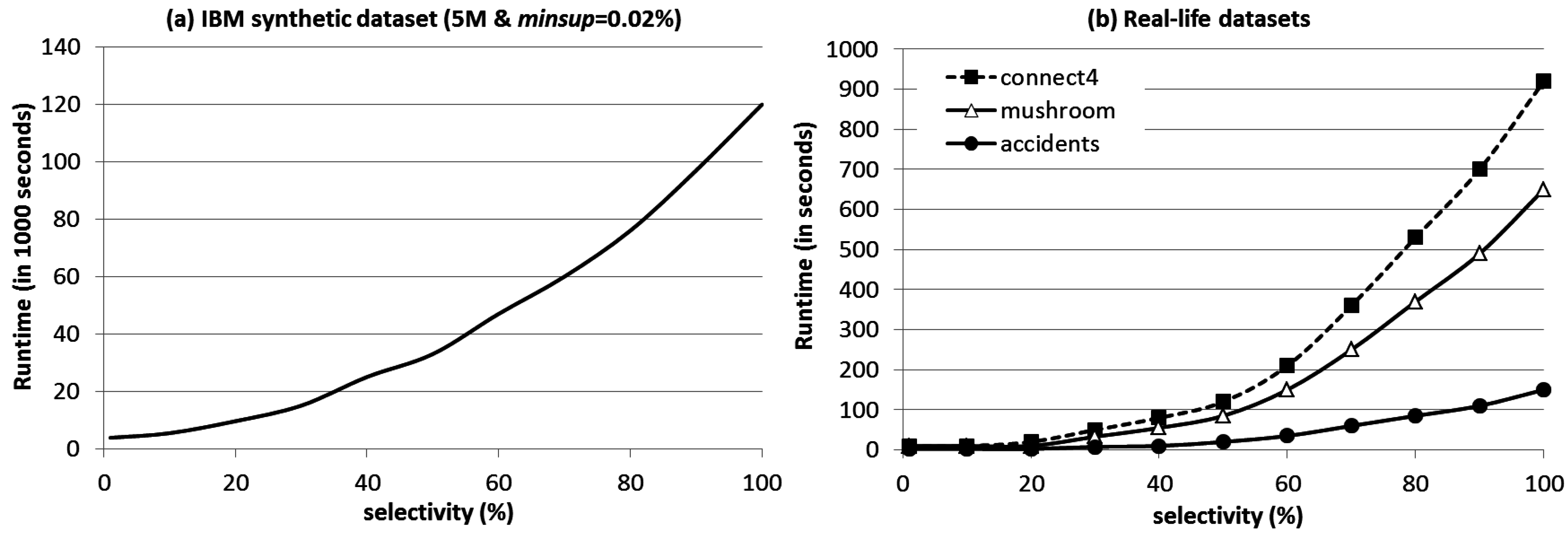
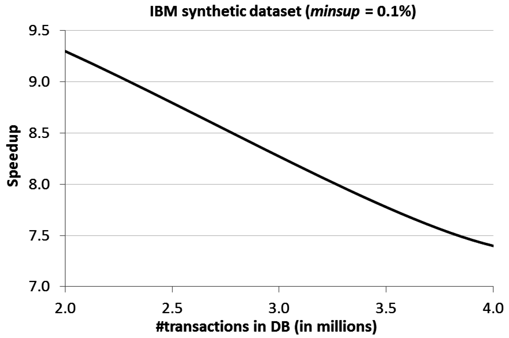
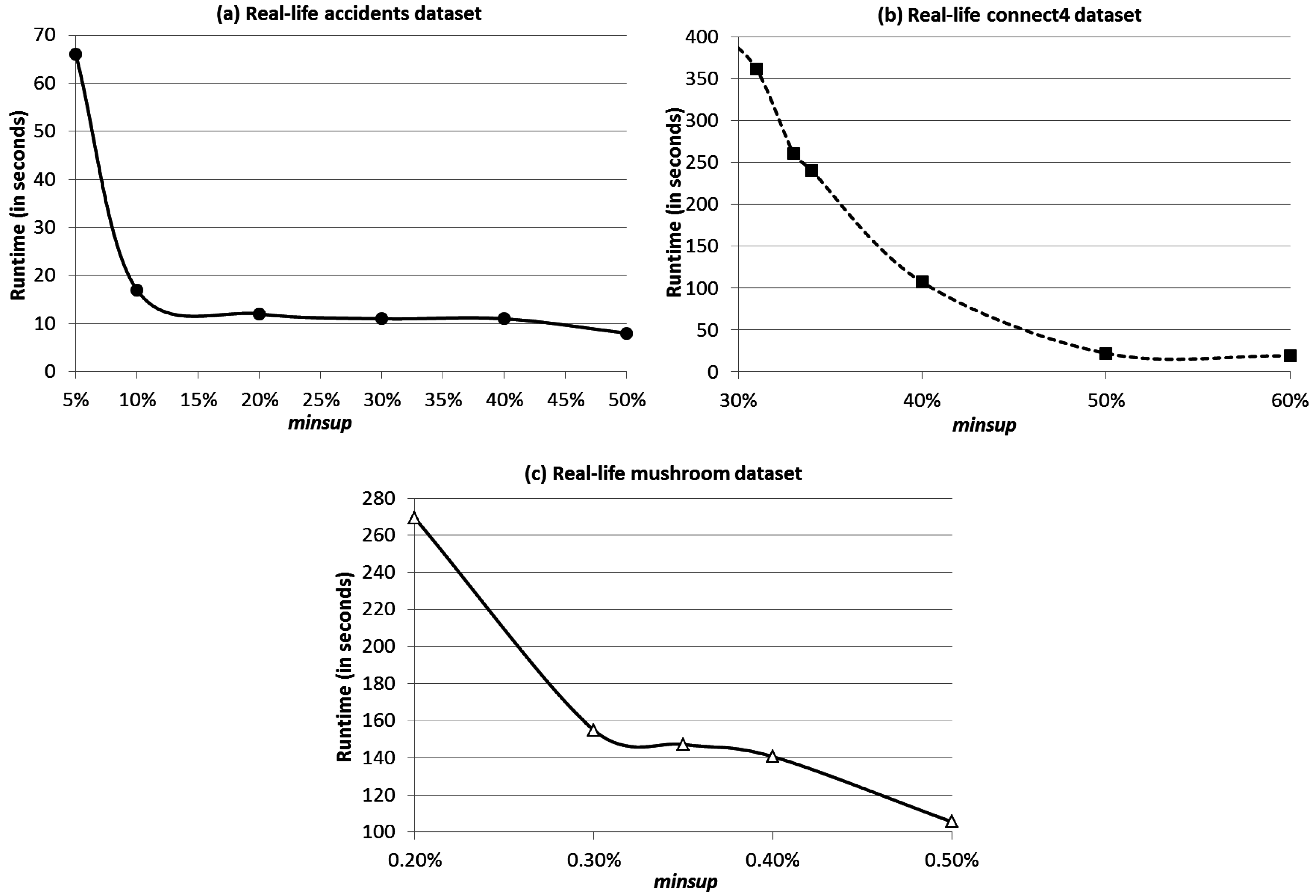
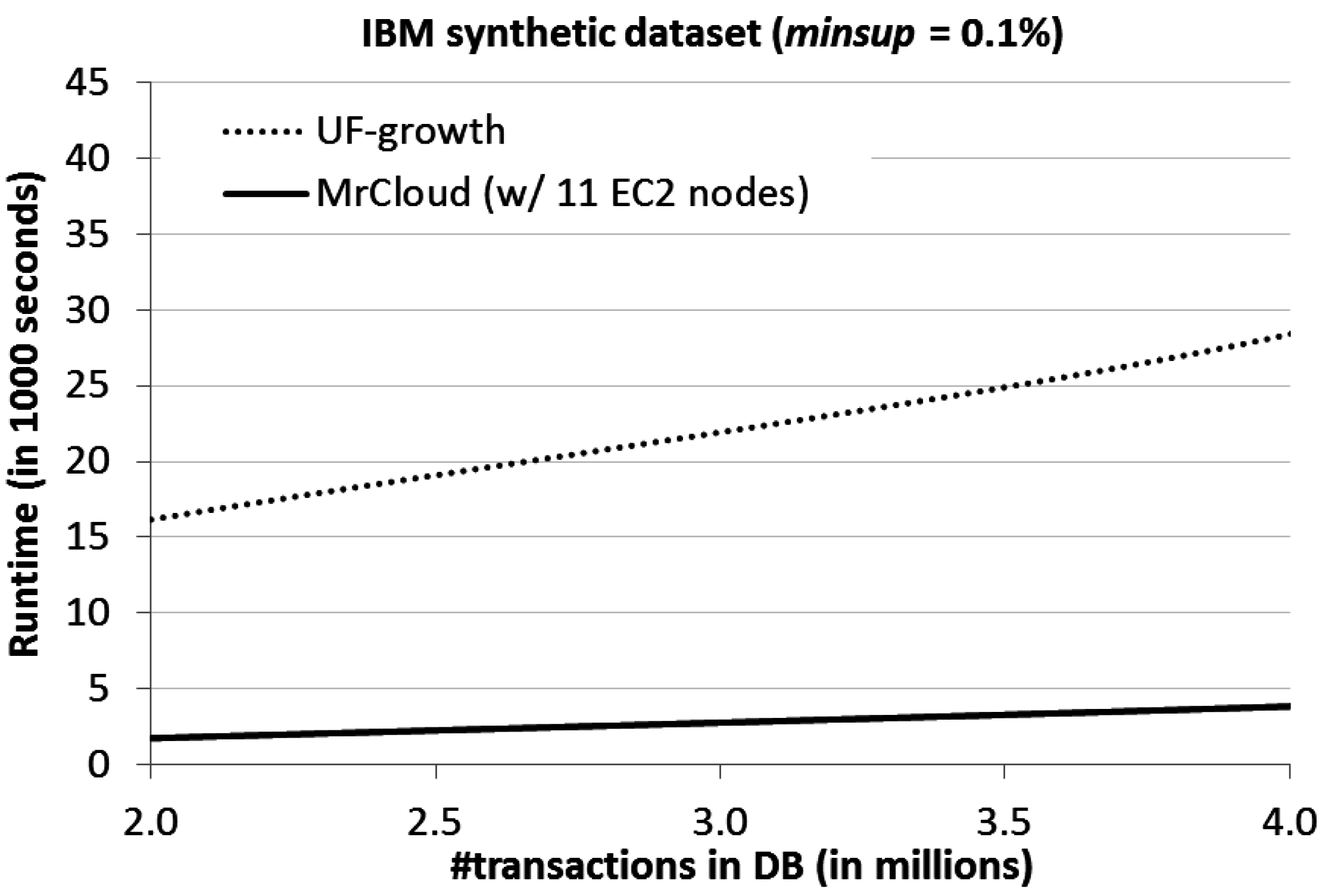
4. Evaluation Results

We evaluated our proposed data analytic algorithm MrCloud in mining user-specified constraints from uncertain big data. We used various benchmark datasets, which include real-life datasets (e.g., accidents, connect4, and mushroom) from the UCI Machine Learning Repository (http://archive.ics.uci.edu/ml/) and the FIMI Repository (http://fimi.ua.ac.be/). We also used IBM synthetic datasets, which were generated using the IBM Quest Dataset Generator [22]. For our experiments, the generated data ranges from 2 M to 10 M transactions with an average transaction length of 10 items from a domain of 1 K items. As the above real-life and synthetic datasets originally contained only precise data, we assigned to each item contained in every transaction an existential probability from the range (0, 1.0]. All experiments were run using either (i) a single machine with an Intel Core i7 4-core processor (1.73 GHz) and 8 GB of main memory running a 64-bit Windows 7 operating system; or (ii) the Amazon Elastic Compute Cloud (EC2) cluster—specifically, 11 High-Memory Extra Large (m2.xlarge) computing nodes (http://aws.amazon.com/ec2/). We implemented existing mining framework [35,39,40], UF-growth [32], tube-growth [33], BLIMP-growth [34], and our data analytic algorithm MrCloud all in the Java programming language. The stock version of Apache Hadoop 0.20.0 was used.

First, we demonstrated the functionality and capability of MrCloud by using (i) a database consisting of items all with existential probability value of 1.0 (indicating that all items are definitely present in the database); and (ii) a user-specified AM constraint. Experimental results show that, in terms of accuracy, our data analytic algorithm returned the same collection of valid frequent patterns as those returned by the existing mining framework [35,39,40] for finding valid frequent patterns from precise data. Note that, in terms of flexibility, MrCloud is not confined to finding valid frequent patterns from a database in which existential probability values of all items are 1.0. MrCloud is capable of finding valid frequent patterns from any database, in which existential probability values of all items are ranging from 0 to 1.0.

Moreover, we also experimented with (i) an uncertain database; and (ii) a user-specified AM constraint with 100% selectivity (so that every item is selected). Experimental results show that, in terms of accuracy, MrCloud returned the same collection of frequent patterns as those returned by UF-growth [32], tube-growth [33] and BLIMP-growth [34]. Note that, in terms of flexibility, MrCloud is not confined to handling AM constraints with 100% selectivity. MrCloud is capable of handling AM constraints with any selectivity.

Afterwards, we demonstrated the efficiency of MrCloud. Figure 1 shows that MrCloud took much shorter runtimes than the runtimes required by the existing UF-growth algorithm [32] when handling AM constraints with 100% selectivity because UF-growth was not designed to handle different selectivity of constraints. Hence, for a fair comparison, we used 100% selectivity for this experiment. We will show in Figure 2 how the runtimes for MrCloud decreased when the selectivity increased (i.e., fewer patterns were selected). For the current experiment, MrCloud was run in the aforementioned EC2 cluster. As a MapReduce-based algorithm, MrCloud takes advantage of all 11 nodes in the EC2 cluster. In contrast, as a non-MapReduce-based algorithm, UF-growth was run on a single machine (i.e., does not take advantage of multiple nodes.) This explains why MrCloud is faster than UF-growth. Moreover, the figure shows the scalability of MrCloud. When the number of transactions in the IBM synthetic dataset increased, the runtimes required by both MrCloud and UF-growth also increased. However, MrCloud required significantly lower runtimes than UF-growth. The same comments apply to other tested datasets (e.g., real-life accidents, connect4, and mushroom datasets).

Figure 1. Runtime vs. #transactions.

Figure 1. Runtime vs. #transactions.

Figure 2. Runtime vs. selectivity on (a) synthetic dataset; and (b) real-life datasets.

Figure 2. Runtime vs. selectivity on (a) synthetic dataset; and (b) real-life datasets.

Figure 2a shows the benefits of constraint pushing in the big data mining process than applying constraint pushing as a post-processing step in the IBM synthetic dataset, while Figure 2b shows those for the three real-life accidents, connect4, and mushroom datasets. Both figures show that, when selectivity decreased (i.e., fewer frequent patterns satisfy the constraints), runtimes also decreased, because (i) fewer pairs were returned by the map function; (ii) fewer pairs were shuffled and sorted by the reduce function; and/or (iii) fewer constraint checks were performed.

Figure 3 shows that MrCloud led to high speedup (e.g., more than 7 times for the IBM synthetic dataset) even with just 11 nodes when compared with UF-growth [32].

Figure 3. Speedup vs. #transactions.

Figure 3. Speedup vs. #transactions.

Figure 4. Runtime vs. minsup on (a) accidents; (b) connect4; and (c) mushroom datasets.

Figure 4. Runtime vs. minsup on (a) accidents; (b) connect4; and (c) mushroom datasets.

Figure 4a shows the efficiency of MrCloud for the real-life accidents dataset: The runtimes of MrCloud decreased when the user-specified minsup increased. Consistent results are shown on Figure 4b and Figure 4c for the real-life connect4 and mushroom datasets, respectively.

5. Conclusions

Big data are everywhere. Existing big data analytic algorithms discover frequent patterns from precise databases. However, there are situations in which data are uncertain. As items in each transaction of these uncertain data are usually associated with existential probabilities expressing the likelihood of these items to be present in the transaction, the corresponding search space for uncertain data is much larger than that for from precise data. This matter is worsened when we are dealing with uncertain big data. Furthermore, in many real-life applications, users may be interested in only a tiny portion of this large search space. To avoid wasting lots of time and space in first discovering all frequent patterns and then pruning uninteresting ones at a post-processing step, we presented in this article a data analytic algorithm called MrCloud that manages uncertain big data, allows users to query these uncertain big data by expressing their interest, and processes the user-specified query by using the MapReduce model in cloud environments. As an output, MrCloud discovers from uncertain big data all and only those patterns that are interesting to the users. Experimental results show the effectiveness of our data analytic algorithm for managing, querying, and processing uncertain big data in cloud environments.

References

1. Cuzzocrea, A.; Saccà, D.; Ullman, J.D. Big Data: A Research Agenda. In Proceedings of the 17th International Database Engineering & Applications Symposium (IDEAS), Barcelona, Spain, 9–11 October 2013; pp. 198–203.
2. Kejariwal, A. Big Data Challenges: A Program Optimization Perspective. In Proceedings of the Second International Conference on Cloud and Green Computing (CGC), Xiangtan, China, 1–3 November 2012; pp. 702–707.
3. Madden, S. From Databases to Big Data. IEEE Int. Comput. 2012, 16, 4–6. [Google Scholar] [CrossRef]
4. Cuzzocrea, A.; Bellatreche, L.; Song, I.-Y. Data Warehousing and OLAP over Big Data: Current Challenges and Future Research Directions. In Proceedings of the 16th International Workshop on Data Warehousing and OLAP (DOLAP), San Francisco, CA, USA, 28 October 2013; pp. 67–70.
5. Jiang, F.; Kawagoe, K.; Leung, C.K. Big Social Network Mining for “Following” Patterns. In Proceedings of the Eighth International C* Conference on Computer Science & Software Engineering (C3S2E), Yokohama, Japan, 13–15 July 2015; pp. 28–37.
6. Kawagoe, K.; Leung, C.K. Similarities of Frequent Following Patterns and Social Entities. Proced. Comput. Sci. 2015, 60, 642–651. [Google Scholar] [CrossRef]
7. Leung, C.K.; Jiang, F. Big Data Analytics of Social Networks for the Discovery of “Following” Patterns. In Proceedings of the 17th International Conference on Big Data Analytics and Knowledge Discovery (DaWaK), Valencia, Spain, 1–4 September 2015; pp. 123–135.
8. Ting, H.-F.; Lee, L.-K.; Chan, H.-L.; Lam, T.W. Approximating Frequent Items in Asynchronous Data Stream over a Sliding Window. Algorithms 2011, 4, 200–222. [Google Scholar] [CrossRef]
9. Kumar, A.; Niu, F.; Ré, C. Hazy: Making It Easier to Build and Maintain Big-Data Analytics. Commun. ACM 2013, 56, 40–49. [Google Scholar] [CrossRef]
10. Leung, C.K.; Hayduk, Y. Mining Frequent Patterns from Uncertain Data with MapReduce for Big Data Analytics. In Proceedings of the 18th International Conference on Database Systems for Advanced Applications (DASFAA), Part I, Wuhan, China, 22–25 April 2013; pp. 440–455.
11. Leung, C.K.; Jiang, F. A Data Science Solution for Mining Interesting Patterns from Uncertain Big Data. In Proceedings of the IEEE Fourth International Conference on Big Data and Cloud Computing (BDCloud), Sydney, NSW, Australia, 3–5 December 2014; pp. 235–242.
12. Leung, C.K.; MacKinnon, R.K. Reducing the Search Space for Big Data Mining for Interesting Patterns from Uncertain Data. In Proceedings of the 2014 IEEE International Congress on Big Data (BigData Congress), Anchorage, AK, USA, 27 June –2 July 2014; pp. 315–322.
13. Dean, J.; Ghemawat, S. MapReduce: Simplified Data Processing on Large Clusters. Commun. ACM 2008, 51, 107–113. [Google Scholar] [CrossRef]
14. Cuzzocrea, A.; Leung, C.K.; MacKinnon, R.K. Mining Constrained Frequent Itemsets from Distributed Uncertain Data. Future Generation Comput. Syst. 2014, 37, 117–126. [Google Scholar] [CrossRef]
15. Leung, C.K.; MacKinnon, R.K.; Jiang, F. Distributed Uncertain Data Mining for Frequent Patterns Satisfying Anti-Monotonic Constraints. In Proceedings of the IEEE 28th International Conference on Advanced Information Networking and Applications (AINA) Workshops, Victoria, BC, Canada, 13–16 May 2014; pp. 1–6.
16. Zaki, M.J. Parallel and Distributed Association Mining: A Survey. IEEE Concurr. 1999, 7, 14–25. [Google Scholar] [CrossRef]
17. Ibrahim, A.; Jin, H.; Yassin, A.; Zou, D. Towards Privacy Preserving Mining over Distributed Cloud Databases. In Proceedings of the Second International Conference on Cloud and Green Computing (CGC), Xiangtan, China, 1–3 November 2012; pp. 130–136.
18. Ismail, L.; Zhang, L. Modeling and Performance Analysis to Predict the Behavior of a Divisible Load Application in a Cloud Computing Environment. Algorithms 2012, 5, 289–303. [Google Scholar] [CrossRef]
19. Wang, L.; Wang, Y.; Xie, Y. Implementation of a Parallel Algorithm Based on a Spark Cloud Computing Platform. Algorithms 2015, 8, 407–414. [Google Scholar] [CrossRef]
20. Alvi, A.K.; Zulkernine, M. A Natural Classification Scheme for Software Security Patterns. In Proceedings of the IEEE Ninth International Conference on Dependable, Autonomic and Secure Computing (DASC), Sydney, NSW, Australia, 12–14 December 2011; pp. 113–120.
21. Meng, Q.; Kennedy, P.J. Determining the Number of Clusters in Co-Authorship Networks Using Social Network Theory. In Proceedings of the Second International Conference on Cloud and Green Computing (CGC), Xiangtan, China, 1–3 November 2012; pp. 337–343.
22. Agrawal, R.; Srikant, R. Fast Algorithms for Mining Association Rules. In Proceedings of the 20th International Conference on Very Large Data Bases (VLDB), Santiago de Chile, Chile, 12–15 September 1994; pp. 487–499.
23. Fariha, A.; Ahmed, C.F.; Leung, C.K.; Samiullah, M.; Pervin, S.; Cao, L. A New Framework for Mining Frequent Interaction Patterns from Meeting Databases. Eng. Appl. Artif. Intell. 2015, 45, 103–118. [Google Scholar] [CrossRef]
24. Cameron, J.J.; Cuzzocrea, A.; Jiang, F.; Leung, C.K. Frequent Pattern Mining from Dense Graph Streams. In Proceedings of the Workshops of the EDBT/ICDT 2014 Joint Conference, Athens, Greece, 28 March 2014; pp. 240–247.
25. Chorley, M.J.; Colombo, G.B.; Allen, S.M.; Whitaker, R.M. Visiting Patterns and Personality of Foursquare Users. In Proceedings of the IEEE Third International Conference on Cloud and Green Computing (CGC), Karlsruhe, Germany, 30 September–2 October 2013; pp. 271–276.
26. Cuzzocrea, A.; Jiang, F.; Lee, W.; Leung, C.K. Efficient Frequent Itemset Mining from Dense Data Streams. In Proceedings of the 16th Asia-Pacific Web Conference (APWeb), Changsha, China, 5–7 September 2014; pp. 593–601.
27. Cameron, J.J.; Leung, C.K. Mining Frequent Patterns from Precise and Uncertain Data. Comput. Syst. J. 2011, 1, 3–22. [Google Scholar]
28. Cuzzocrea, A.; Furfaro, F.; Saccà, D. Hand-OLAP: A System for Delivering OLAP Services on Handheld Devices. In Proceedings of the Sixth International Symposium on Autonomous Decentralized Systems (ISADS), Pisa, Italy, 9–11 April 2003; pp. 80–87.
29. Leung, C.K.; MacKinnon, R.K. Balancing Tree Size and Accuracy in Fast Mining of Uncertain Frequent Patterns. In Proceedings of the 17th International Conference on Big Data Analytics and Knowledge Discovery (DaWaK), Valencia, Spain, 1–4 September 2015; pp. 57–69.
30. Tong, W.; Leung, C.K.; Liu, D.; Yu, J. Probabilistic Frequent Pattern Mining by PUH-Mine. In Proceedings of the 17th Asia-Pacific Web Conference (APWeb), Guangzhou, China, 18–20 September 2015; pp. 781–793.
31. Tong, Y.; Chen, L.; Cheng, Y.; Yu, P.S. Mining Frequent Itemsets over Uncertain Databases. PVLDB 2012, 5, 1650–1661. [Google Scholar] [CrossRef]
32. Leung, C.K.; Mateo, M.A.F.; Brajczuk, D.A. A Tree-Based Approach for Frequent Pattern Mining from Uncertain Data. In Proceedings of the 12th Pacific-Asia Conference on Knowledge Discovery and Data Mining (PAKDD), Osaka, Japan, 20–23 May 2008; pp. 653–661.
33. Leung, C.K.; MacKinnon, R.K.; Tanbeer, S.K. Fast Algorithms for Frequent Itemset Mining from Uncertain Data. In Proceedings of the IEEE 14th International Conference on Data Mining (ICDM), Shenzhen, China, 14–17 December 2014; pp. 893–898.
34. Leung, C.K.; MacKinnon, R.K. BLIMP: A Compact Tree Structure for Uncertain Frequent Pattern Mining. In Proceedings of the 16th International Conference on Data Warehousing and Knowledge Discovery (DaWaK), Munich, Germany, 2–4 September 2014; pp. 115–123.
35. Ng, R.T.; Lakshmanan, L.V.S.; Han, J.; Pang, A. Exploratory Mining and Pruning Optimizations of Constrained Associations Rules. In Proceedings of the 1998 ACM SIGMOD International Conference on Management of Data, Seattle, WA, USA, 2–4 June 1998; pp. 13–24.
36. Jiang, F.; Leung, C.K.; MacKinnon, R.K. BigSAM: Mining Interesting Patterns from Probabilistic Databases of Uncertain Big Data. In Proceedings of the PAKDD 2014 International Workshops, Tainan, Taiwan, 13–16 May 2014; pp. 780–792.
37. Lin, M.-Y.; Lee, P.-Y.; Hsueh, S.-C. Apriori-Based Frequent Itemset Mining Algorithms on MapReduce. In Proceedings of the ACM Sixth International Conference on Ubiquitous Information Management and Communication (ICUIMC), Kuala Lumpur, Malaysia, 20–22 February 2012. [CrossRef]
38. Riondato, M.; DeBrabant, J.; Fonseca, R.; Upfal, E. PARMA: A Parallel Randomized Algorithm for Approximate Association Rules Mining in MapReduce. In Proceedings of the ACM 21st International Conference on Information and Knowledge Management (CIKM), Maui, HI, USA, 29 October–2 November 2012; pp. 85–94.
39. Lakshmanan, L.V.S.; Leung, C.K.; Ng, R.T. Efficient Dynamic Mining of Constrained Frequent Sets. ACM Trans. Database Syst. 2003, 28, 337–389. [Google Scholar] [CrossRef]
40. Leung, C.K. Frequent Itemset Mining with Constraints. In Encyclopedia of Database Systems; Springer: New York, NY, USA, 2009; pp. 1179–1183. [Google Scholar]
41. Leung, C.K. Uncertain Frequent Pattern Mining. In Frequent Pattern Mining; Springer International Publishing: Cham, Switzerland, 2014; pp. 417–453. [Google Scholar]
42. Leung, C.K. Mining Frequent Itemsets from Probabilistic Datasets. In Proceedings of the Fifth International Conference on Emerging Databases (EDB), Jeju Island, South Korea, 19–21 August 2013; pp. 137–148.