Effective Data Acquisition Protocol for Multi-Hop Heterogeneous Wireless Sensor Networks Using Compressive Sensing

Abstract

In designing wireless sensor networks (WSNs), it is important to reduce energy dissipation and prolong network lifetime. Clustering of nodes is one of the most effective approaches for conserving energy in WSNs. Cluster formation protocols generally consider the heterogeneity of sensor nodes in terms of energy difference of nodes but ignore the different transmission ranges of them. In this paper, we propose an effective data acquisition clustered protocol using compressive sensing (EDACP-CS) for heterogeneous WSNs that aims to conserve the energy of sensor nodes in the presence of energy and transmission range heterogeneity. In EDACP-CS, cluster heads are selected based on the distance from the base station and sensor residual energy. Simulation results show that our protocol offers a much better performance than the existing protocols in terms of energy consumption, stability, network lifetime, and throughput.

1. Introduction

With rapid advancement in electronics industry, small inexpensive battery-powered wireless sensors have already started to make an impact on the communication with the physical world. WSN consists of large number of low cost devices to gather information from the diverse kinds of physical phenomenon. The sensors can monitor various entities such as: temperature, pressure, humidity, salinity, metallic objects, and mobility; this monitoring capability can be effectively used in commercial, military, and environmental applications [1,2,3,4,5,6,7,8,9,10,11]. For these sensor network applications, most research has discussed problems by the deployment of large number of low-cost homogeneous devices. But in practical applications, in order to meet the demands of various applications for the technologies of sensor networks, increasing attentions have been attracted to the researches on heterogeneous WSNs [12]. Heterogeneous WSN is composed of different types of sensor nodes, which are in a wide range of applications [13,14]. In fact, the heterogeneity is common in the WSNs [15]. The priority should be given to reduce energy dissipation in network operation, improve network load and stability, and prolong network lifetime.

Compressive sensing (CS) [16,17,18] is a collection of recently proposed sampling methods in information theory. The combination of CS theory with WSNs holds promising improvements to the lifetime of wireless sensors, whereas it reduces global scale communication cost without introducing intensive computation or complicated transmission control. CS states that sparse signal of information in WSNs can be exactly reconstructed from a small number of random linear measurements of information in WSNs [19]. CS provides a new approach to mathematical complexities especially when sparse information is applied. CS tends to recover data vector $X\in {\mathbb{R}}^N$ with N number of information form data vector $Y\in {\mathbb{R}}^M$ with M number of information such that $M\ll N$ [20]. This will result in extending the lifetime of the sensor network.

Energy consumption in networks can be effectively reduced by organizing clustering sensor nodes, so many energy-efficient routing protocols are designed on the basis of the clustering structure. Currently, a number of distributed clustering protocols are proposed. In accordance with the networks, homogeneous or heterogeneous, to which the protocols are adaptive, clustering protocols can be categorized into homogeneous clustering protocols which assume that all the sensor nodes are identical and heterogeneous clustering protocols which assume that the sensor nodes have different capabilities. Due to the dynamic and complex nature of energy configuration and network evolution, it is very difficult to design a clustering protocol which can save energy and provide reliable data transmission in heterogeneous networks.

To overcome the above problems, we propose a new protocol EDACP-CS for heterogeneous WSNs. EDACP-CS includes two phases: the cluster head arrangement phase and the routing phase. In cluster head arrangement phase, all the sensor nodes organize themselves into clusters with one node elected as a cluster head (CH) according to their weighted election probabilities and their distance to the base station (BS) to determine near nodes and far nodes in order to give more chance to nearest nodes to be CHs by modifying the election probability value for each type of nodes. In the routing phase, after receiving the data from the member nodes, each CH compresses the collected data using CS and transfers it to the BS. Simulation results show that our protocol can aggregate data efficiently and reduce energy consumption greatly, prolonging the stability period and the lifetime of the whole network strongly depend on higher values of extra energy during its heterogeneous settings and different transmission ranges.

The remainder of the paper is organized as follows: Section 2 presents the related work of the proposed protocol. In Section 3, we introduce the proposed system model. Simulation results and its discussion are presented in Section 4. Finally, the conclusion of our work is given in Section 5.

2. Related Work

Recently there has been a growing interest in WSNs. One of the major issues in WSN is developing an energy-efficient routing protocol. Since the sensor nodes have limited available power, energy conservation is a critical issue in WSN for nodes and network life. The issue of heterogeneity (in terms of energy) of nodes is addressed in [21]. In [22], the proposed protocol is based on random selection of CHs weighted according to the remaining energy of the node. This approach addresses the problem of varying energy levels and consumption rates but still assumes that the BS can be reached directly by all the nodes.

In [23], the authors provided the optimal heterogeneous sensor deployment that minimizes the deployment cost in different communication modes. In their model, the cost of the cluster head device is determined by the amount of initial battery energy, which depends on the number of cluster members and communication mode. They do not consider the sensing coverage and aging process over time.

Low-Energy Adaptive Clustering Hierarchy (LEACH) [9] is one of the most popular distributed cluster-based routing protocols in WSNs. The operation of LEACH is generally separated into two phases, the set-up phase and the steady-state phase. In the set-up phase, CHs are selected and clusters are organized, each node decides whether to become a CH for the current round. This decision is based on a predetermined fraction of nodes and the threshold $T\left(s\right)$, which is given by:

$$T\left(s\right)=\left\{\begin{array}{cc}\frac{p_{opt}}{\left(1-p_{opt}\times \left(rmod\left(1/p_{opt}\right)\right)\right)}\hfill & \text{if}s\in G,\hfill \\ 0\hfill & otherwise,\hfill \end{array}\right.$$

(1)

where $p_{opt}$ is the predetermined percentage of CHs, r is the count of current round and G is the set of sensor nodes that have not been CHs in the last $1/p_{opt}$ rounds. Using this threshold, each node will be a CH at a round within $1/p_{opt}$ rounds. After $1/p_{opt}$ rounds, all nodes are once again eligible to become CHs. In this way, the energy concentration on CHs is distributed. LEACH does not consider the residual energy of each node so the nodes that have relatively smaller energy remaining can be selected as CHs. This makes the network lifetime shortened. In the steady-state phase, the actual data transmissions to the BS take place. After the steady-state phase, the next round begins.

In [24], the authors proposed a new routing protocol and data aggregation method in Leach-heterogeneous system where the sensor nodes form the cluster and the CH elected based on the residual energy of the individual node calculation with re-clustering scheme is adopted in each cluster of the WSNs. The proposed protocol works with 3 types of nodes (normal, advanced and super), CHs are selected on the basis of their residual energy and their distances to the BS.

CS is a novel sensing/sampling paradigm that goes against the common wisdom in data acquisition, the theory of CS extends traditional sensing and sampling systems to a much broader class of signals. The promise of CS is that a sparse or compressible signal can be recovered from a small salient set of projections. To make this possible, there are two principles [16]: sparsity, which pertains to the signals of interest, and incoherence, which pertains to the sensing modality. Under CS framework, any compressible signal $X\in {\mathbb{R}}^N$ can be represented in the form of:

$$X=\Psi \alpha ,$$

(2)

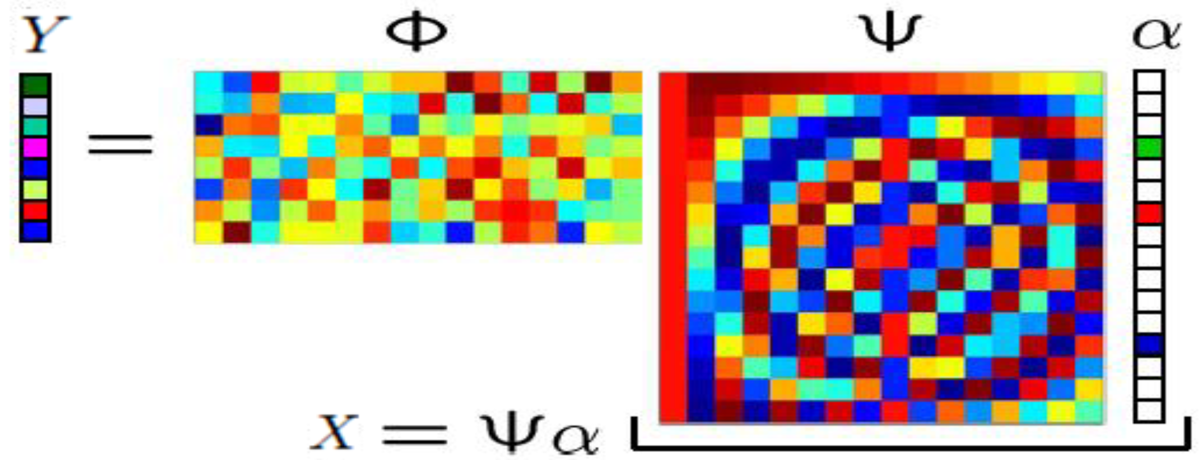
where $\Psi \in {\mathbb{R}}^{N\times N}$ is the transform matrix and α is the sparse representation of X. There are no more than K nonzero entries in vector α, where K is much smaller than N, and the signal X is called K sparse signal. In contradiction to sparsity, incoherence means that the measurement matrix Φ has dense representation in basis Ψ, and Φ is independent to Ψ. In practice, most of natural signals are sparse or near sparse, and they can be recovered from their compressible samples. For a signal $X\in {\mathbb{R}}^N$, we can obtain its M linear observations, as in Figure 1.

$$Y=\Phi X=\Phi \Psi \alpha ,$$

(3)

Figure 1. The scheme of compressive sampling.

Figure 1. The scheme of compressive sampling.

If $\Theta =\Phi \Psi$ satisfies the restricted isometry property (RIP) [16], condition $M\le cKlog(N/K)$ such that c is a small constant with $c>0$, the vector α can be accurately recovered from Y as the unique solution of:

$$\widehat{\alpha }=argmi{n}_{\alpha }{∥\alpha ∥}_{1}s.t.Y=\Phi \Psi \alpha ,$$

(4)

The original networked data X may be sparse itself or can be sparsified with a suitable transform such as Discrete Cosine Transform or Discrete Wavelet transform [25,26,27]. One example of the self-sparse X is a linear combination of just K basis vectors, with $K\ll N$, that is; only K are nonzero and $(N-K)$ are zero [28]. Usually, the networked data vector X is sparse with a proper Ψ in Equation (2). Most of the previous works [25,26,27] consider a regular sensor network. However, sensors are usually deployed on an irregular grid. So it is expected to find some sparse representations to sparsify irregular grid sensor networked data. In WSNs, sampling matrix Φ is usually pre-designed, i.e., each sensor locally draws M elements of the random projection vectors by using its network address as the seed of a pseudorandom number generator. Based on CS theory, Jia et al. [28] considers a sparse event detection scenario where the channel impulse response (CIR) matrix is used as a natural sampling matrix. In [29], a basic global superposition model to obtain the measurements of sensor data is proposed, where a sampling matrix is modeled as the channel impulse response (CIR) matrix while the sparsifying matrix is expressed as the distributed wavelet transform. In [30], compressive distributed sensing using random walk CDS(RW) algorithm is proposed that uses rateless coding. In our proposed protocol we use CS to fuse data efficiently in EDACP-CS and consider three types of nodes and different transmission ranges to achieve a robust self configured WSN that maximizes lifetime.

In [31], energy efficient clustering and data aggregation protocol for heterogeneous WSNs (EECDA) has been proposed. EECDA combines energy efficient cluster based routing and data aggregation for improving the performance in terms of lifetime and stability. However, in the proposed protocol we discuss effectively the aggregation using CS and consider the heterogeneity of nodes due to energy as well as transmission ranges. We assume that CHs are randomly selected based on their residual energy and the distance form the BS. 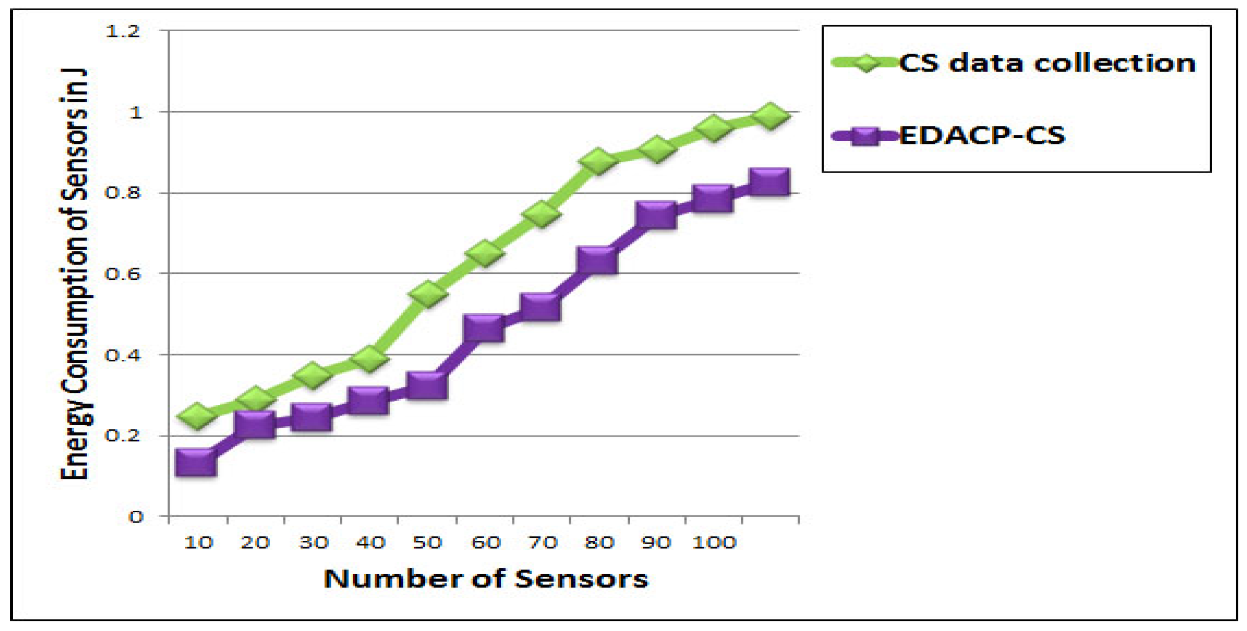In [32], the authors have proposed a novel data collection algorithm using compressive sensing (CS data collection). In CS data collection, each sensor node only communicates with its neighbor node in one hop. However, in the proposed protocol all sensor nodes organize themselves into clusters with one node elected as a CH based on their weighted election probabilities and their distance to the BS.

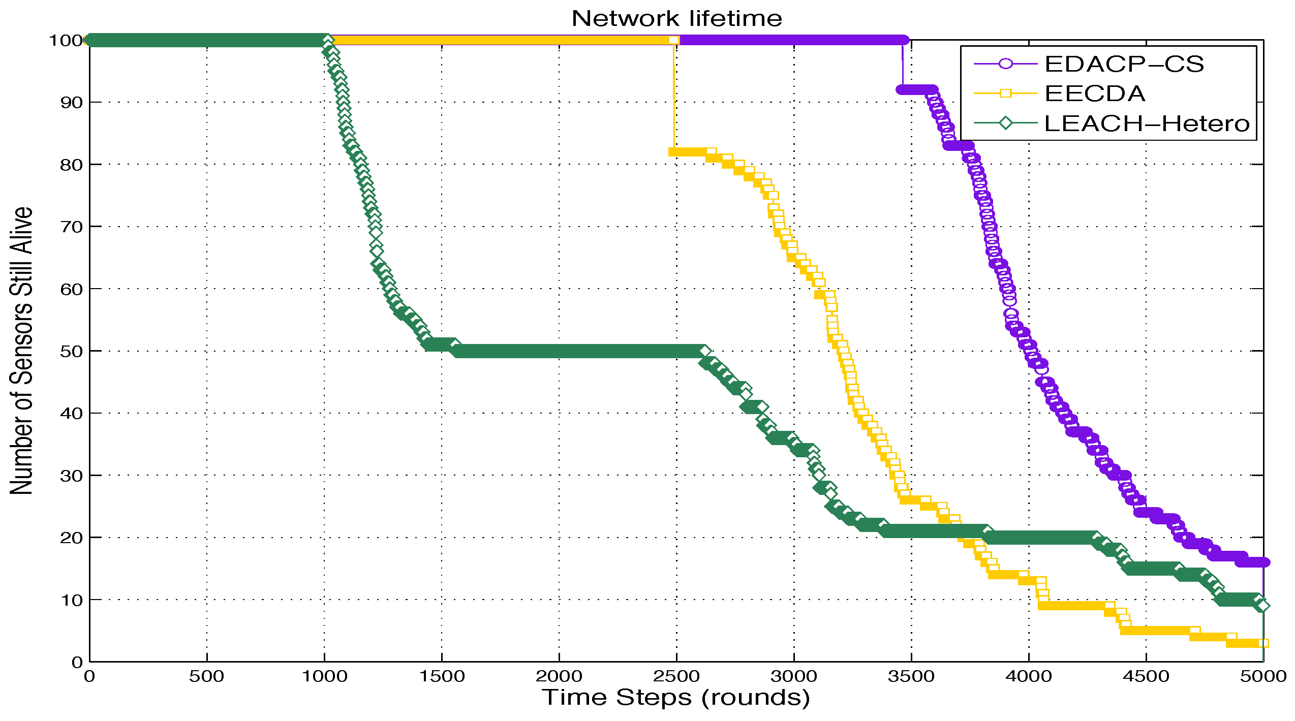
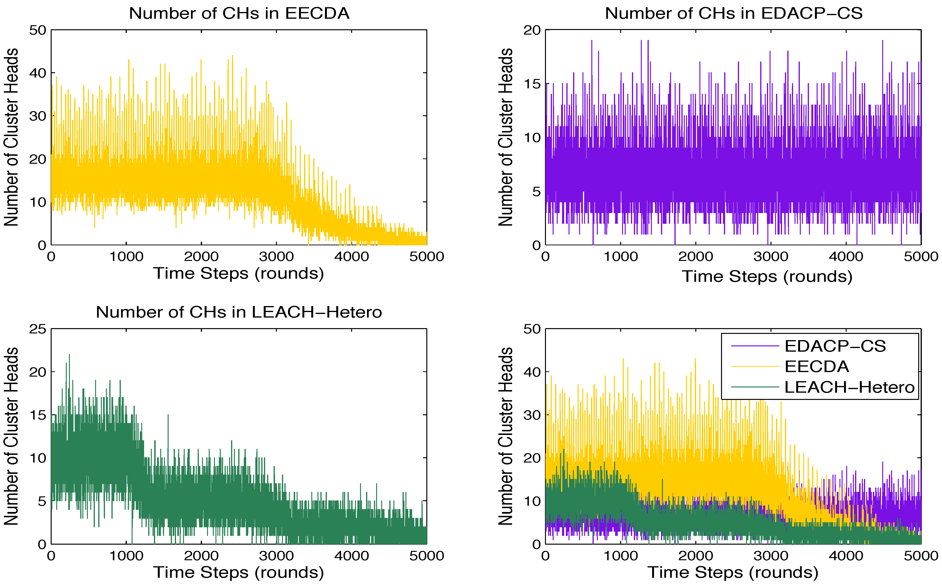
All the above protocols do not consider efficient data compression and link heterogeneity. In the proposed protocol EDACP-CS, each sensor node independently elects itself as a CH based on its residual energy and its distance to the BS. Therefore, nodes that are closer to the BS and contain more energy than the other nodes have more chance to be selected as a CH for current round. EDACP-CS introduces a new scheme to combine clustering strategy with CS theory for increasing both energy and stable period constrains under heterogeneous environment in terms of node energy and transmission range. Simulation shows that the network lifetime and the stability period are much better in the proposed protocol than CS data collection, EECDA and LEACH-Hetero protocols.

3. System Model

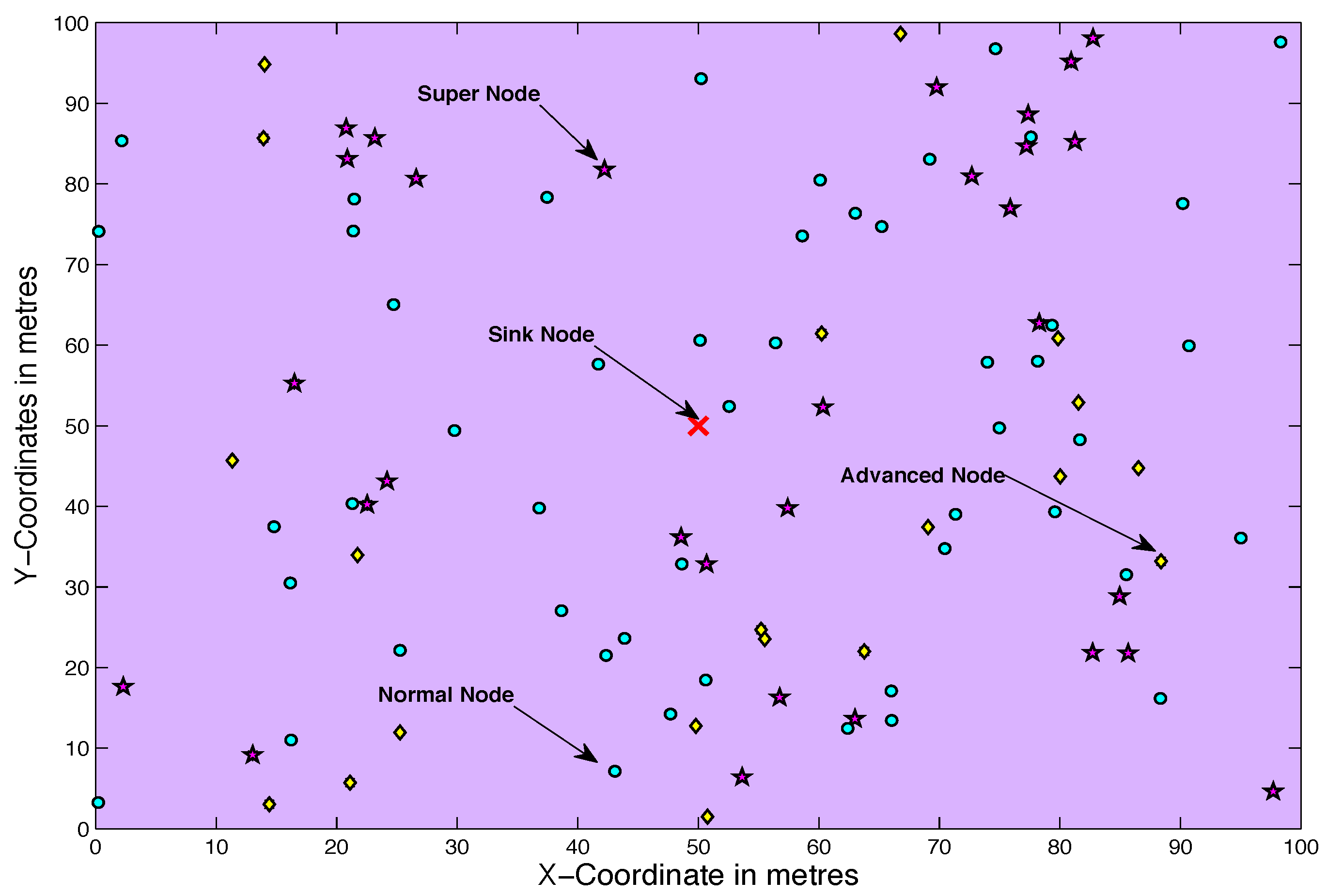
In EDACP-CS protocol, we consider heterogeneous WSN with nodes of different energy levels and transmission ranges. Sensor nodes are divided into three categories (normal, advanced and super) nodes as shown in Figure 2. The energy consumption of advanced is less than that of normal and the energy consumption of super is less than that of advanced.

Figure 2. A heterogeneous wireless sensor network.

Figure 2. A heterogeneous wireless sensor network.

3.1. Network and Energy Model Assumptions

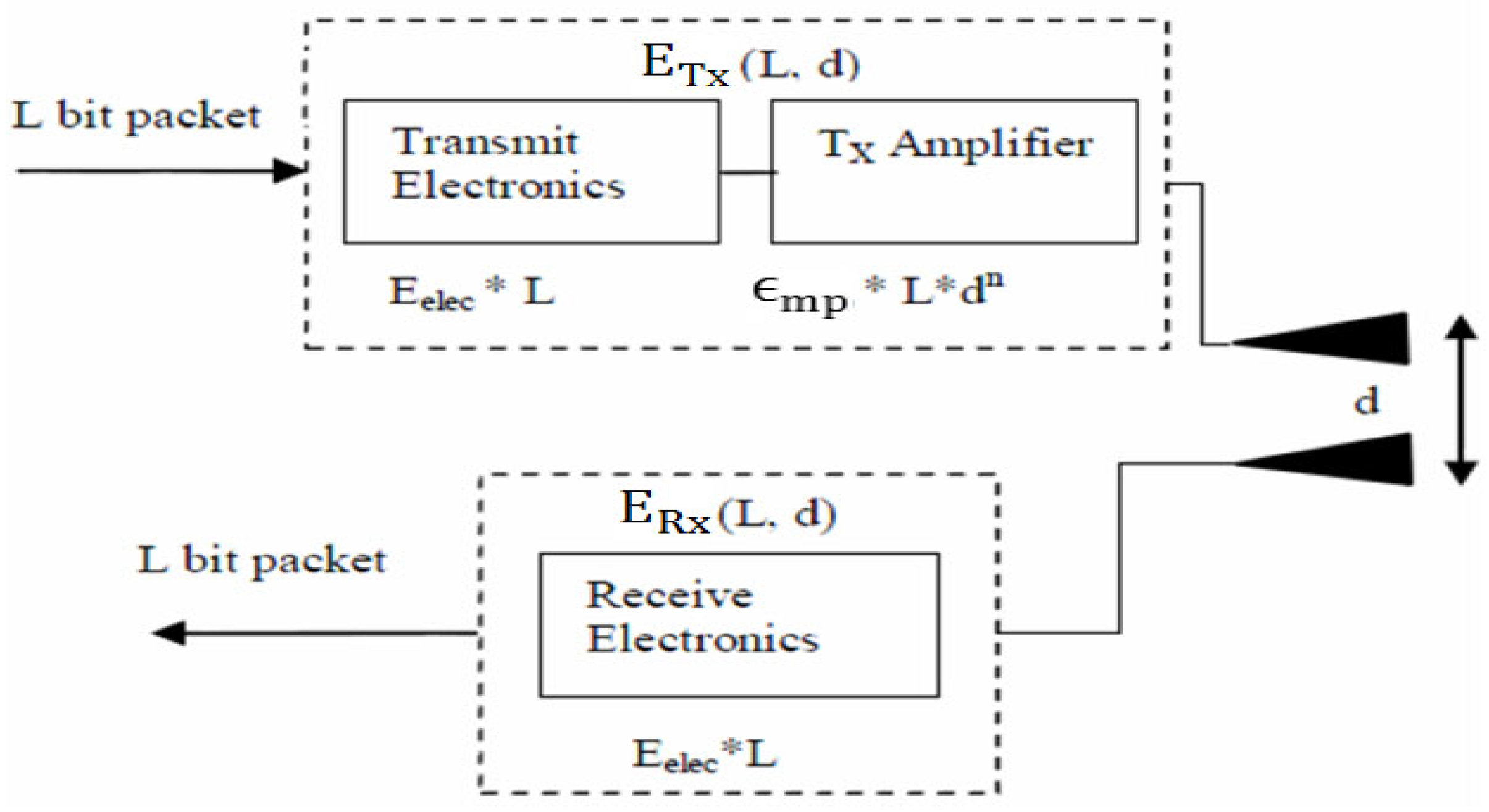
In EDACP-CS, we use the simplified energy model proposed in [33]. According to the radio energy dissipation model illustrated in Figure 3, in order to achieve an acceptable Signal-to-Noise Ratio (SNR) in transmitting an $L-$bit message over a distance d, the energy expended by the radio is given by:

$$E_{Tx}(l,d)=\left\{\begin{array}{cc}L.E_{elec}+L.{ϵ}_{fs}.d^2\hfill & \text{if}d\le d_0,\hfill \\ L.E_{elec}+L.{ϵ}_{mp}.d^4\hfill & \text{if}d>d_0,\hfill \end{array}\right.$$

(5)

where $E_{elec}$ is the energy dissipated per bit to run the transmitter or the receiver circuit, ${ϵ}_{fs}$ and ${ϵ}_{mp}$ depend on the transmitter amplifier model we use, and d is the distance between the sender and the receiver. By equating the two expressions at $d=d_0$, we have $d_0=\sqrt{\frac{{ϵ}_{fs}}{{ϵ}_{mp}}}$. To receive an $L-$bit message the radio expends $E_{Rx}=L.E_{elec}$.

We make some assumptions about the sensor nodes and underlying network model as follows:

• All sensor nodes are stationary and uniformly distributed within a square field,
• Communication among sensor nodes is based on single-hop approach,
• Networked data vector is sparse or highly compressible in Distributed Wavelet Transform (DWT) domain, i.e., it contains K largest coefficients. Setting the rest coefficients zero will not cause much information loss,
• A WSN consists of heterogeneous nodes in terms of node energy and transmission range.

Figure 3. Radio Energy Dissipation Model.

Figure 3. Radio Energy Dissipation Model.

3.2. Optimal Number of Clusters

We assume that an area $A=R\times R$ square meters over which N nodes are uniformly distributed. For simplicity, assume the sink is located in the center of the field, and that the distance between any node to the BS or its CH is $r_p(r_p\le d_0)$, where $d_0$ is the maximum transmission range. We consider that after deployment, the BS broadcasts a “hello” message to all the nodes at a certain power level. Each node can compute its approximated distance $\left(D_i\right)$ to the BS based on the received signal strength. The average distance $D_{avg}$ between nodes and the BS is given by:

$$D_{avg}=\frac{1}{N}\sum _{i=1}^N{D}_i,$$

(6)

The value of $D_{avg}$ can be approximated as:

$$D_{avg}\approx d_{CH}+d_{BS},$$

(7)

where $d_{CH}$ is the average distance between a cluster member and its CH and $d_{BS}$ is the average distance between the CH and the BS. The energy dissipated in the CH node during a round is given by the following formula:

$$E_{CH}=(\frac{N}{C}-1)Y.E_{elec}+\frac{N}{C}Y+Y.E_{elec}+Y.{\mathrm{ϵ}}_{fs}{d}_{BS}^2,$$

(8)

where C is the number of clusters, Y is the compressed data. The energy dissipated by a non-CH node is given by:

$$E_{nonCH}=L.E_{elec}+L.{\mathrm{ϵ}}_{fs}{d}_{CH}^2,$$

(9)

Using Euclidian metric, the area occupied by each cluster will be $\lambda =\frac{R^2}{C}$ with node distribution $\mathrm{\rho }(x,y)$:

$$d_{CH}^2=\int \int (x^2+y^2)\mathrm{\rho }(x,y)dxdy=\int \int r^2\mathrm{\rho }(r,\mathrm{\theta })rdrd\mathrm{\theta },$$

(10)

Assuming the area is a circle with radius $\eta =R/\sqrt{\pi C}$, $\mathrm{\rho }(r,\mathrm{\theta })$ is constant, and the density ρ is uniform where $\mathrm{\rho }=(1/(R^2/C))$, $d_{CH}^2$ can be simplified as follows:

$$d_{CH}^2=\int \int (x^2+y^2)\rho (x,y)dxdy=\mathrm{\rho }{\int }_{\mathrm{\theta }=0}^{2\pi }{\int }_{r=0}^{R/\sqrt{\pi C}}{r}^{3}drd\mathrm{\theta }=\frac{R^2}{2\pi C},$$

(11)

The energy dissipated in a cluster per round is given by:

$$E_{cluster}\approx E_{CH}+\frac{N}{C}{E}_{nonCH},$$

(12)

The total energy dissipation in the network per round will be the sum of the energy dissipation by all clusters, i.e.,

$$E_{tot}=C{E}_{cluster}=Y(N(1+E_{elec})+C{\mathrm{ϵ}}_{fs}{d}_{BS}^2)+NL(E_{elec}+{\mathrm{ϵ}}_{fs}{d}_{CH}^2),$$

(13)

By differentiating $E_{tot}$ with respect to C and equating to zero, the optimal number of constructed clusters can be found:

$$C_{opt}=\sqrt{\frac{NL}{2\pi Y}}\frac{R}{d_{BS}}=\sqrt{\frac{NL}{2\pi Y}}\frac{2}{0.765},$$

(14)

where, the average distance from a CH to the BS $d_{BS}$ is given by [34] such that $A=R^2$:

$$d_{BS}={\int }_A\sqrt{x^2+y^2}\frac{1}{A}dA=0.765\frac{R}{2},$$

(15)

If the distance of a significant percentage of nodes to the BS is greater than $d_0$ then, following the same analysis as in [33] we will obtain:

$$E_{CH}=(\frac{N}{C}-1)Y.E_{elec}+\frac{N}{C}Y+Y.E_{elec}+Y.{\mathrm{ϵ}}_{mp}{d}_{BS}^4,$$

(16)

By substituting in Equation (13) and differentiating $E_{tot}$ with respect to C and equating to zero, we will find:

$$C_{opt}=\sqrt{\frac{NL}{2\pi Y}}\sqrt{\frac{{ϵ}_{fs}}{{ϵ}_{mp}}}\frac{R}{d_{BS}^2},$$

(17)

The optimal probability of a node to become a CH, $p_{opt}$, can be computed as follows:

$$p_{opt}=\frac{C_{opt}}{N},$$

(18)

The optimal construction of clusters (which is equivalent to the setting of the optimal probability for a node to become a CH) is very important. In [9], the authors showed that if the clusters are not constructed in an optimal way, the total consumed energy of the WSN per round is increased exponentially either when the number of the constructed clusters is greater than the optimal number of clusters or especially when the number of the constructed clusters is less than the optimal number of clusters. If the number of the constructed clusters is less than the optimal number of clusters, some nodes in the network have to transmit their data very far to reach the CH, this will increase the energy of the system. If the number of the constructed clusters is greater than the optimal number of clusters, the total routing traffics within each cluster will be reduced because of fewer members, however, more clusters will result in more than one-hop transmissions from the CHs to the BS also the CHs will receive data from fewer members this will reduce the local data aggregation being performed and increase the communications among the CHs.

3.3. Cluster Head Election Phase

The optimal probability of a node to become a CH is equivalent to the optimal construction of clusters. This clustering is optimal in the sense that energy consumption is well distributed over all sensors and the total energy consumption is minimal. Such optimal clustering highly depends on the energy model that we use.

In EDACP-CS, the nodes with less energy than the others and the nodes with more distance from the BS than the others have the smallest chance to be selected as a CH for current round. Let us assume $E_0$ is the initial energy of each normal sensor node, m is the fraction of advanced nodes among normal nodes which are equipped with α times more energy than the normal nodes, and $m_0$ is the fraction of super nodes among advanced nodes which are equipped with β times more energy than the normal nodes. Note a new heterogeneous setting has no affect on the spatial density of the network so the setting of $p_{opt}$ does not change. On the other hand, due to heterogeneous nodes the net energy of the network is changed as the initial energy of each super node becomes $E_0(1+\beta )$ and each advanced node becomes $E_0(1+\alpha )$. Therefore, the total (initial) energy of the new heterogeneous setting is given by Equation (19):

$$TotalEnergy=N\ast E_0(1+m(\alpha -m_0(\alpha -\beta ))),$$

(19)

Hence, the total energy of the system is increased by a factor of $\mathrm{\mu }=(1+m(\alpha -m_0(\alpha -\beta )))$ In order to optimize the stable region of the system, the new epoch must become equal to $\left(\frac{1}{p_{opt}}\right)\mathrm{\mu }$ because the system has $m(\alpha -m_0(\alpha -\beta ))$ times more energy.

Virtually there are $N\times \mathrm{\mu }$ nodes with energy equal to the initial energy of a normal node. In order to maintain the minimum energy consumption in each round within an epoch, the average number of CHs per round per epoch must be constant and equal to $N\times p_{opt}$. In the heterogeneous scenario the average number of CHs per round per epoch is equal to $\mu \times N\times p_{nrm}$ (because each virtual node has the initial energy of a normal node). Therefore, the weighed probabilities for normal, advanced and super nodes according to residual energy and the distance from the BS are, respectively:

If distance $D_i\le D_{avg}$ we take:

$$p_{nrm}=\frac{p_{opt}}{\mathrm{\mu }}\left(1-\frac{D_i}{D_{avg}}\right),$$

(20)

$$p_{adv}=\frac{p_{opt}}{\mathrm{\mu }}\times (1+\alpha )\left(1-\frac{D_i}{D_{avg}}\right),$$

(21)

$$p_{sup}=\frac{p_{opt}}{\mathrm{\mu }}\times (1+\beta )\left(1-\frac{D_i}{D_{avg}}\right).$$

(22)

Else we keep:

$$p_{nrm}=\frac{p_{opt}}{\mathrm{\mu }},$$

(23)

$$p_{adv}=\frac{p_{opt}}{\mathrm{\mu }}\times (1+\alpha ),$$

(24)

$$p_{sup}=\frac{p_{opt}}{\mathrm{\mu }}\times (1+\beta ).$$

(25)

In Equation (1), we replace $p_{opt}$ by the weighted probabilities to obtain the threshold that is used to elect the CH in each round. We define $T{s}_{nrm}$ as the threshold for normal nodes, $T{s}_{adv}$ the threshold for advanced nodes and $T{s}_{sup}$ the threshold for super nodes. Thus, for normal nodes, we have:

$$T{s}_{nrm}=\left\{\begin{array}{cc}\frac{p_{nrm}}{\left(1-p_{nrm}\times \left(rmod\left(1/p_{nrm}\right)\right)\right)}\hfill & \text{if}{s}_{nrm}\in G^{\prime },\hfill \\ 0\hfill & otherwise,\hfill \end{array}\right.$$

(26)

where r is the current round, $G^{\prime }$ is the set of normal nodes that have not become CHs within the last $1/p_{nrm}$ rounds of the epoch, and $T{s}_{nrm}$ is the threshold applied to a population of $N(1-m)$ normal nodes. This guarantees that each normal node will become a CH exactly once every $\left(\frac{1}{p_{opt}}\right)\mathrm{\mu }$ rounds per epoch, and that the average number of CHs that are normal nodes per round per epoch is equal to $N(1-m)\times p_{nrm}$ Similarly, for advanced and super nodes, we have:

$$T{s}_{adv}=\left\{\begin{array}{cc}\frac{p_{adv}}{\left(1-p_{adv}\times \left(rmod\left(1/p_{adv}\right)\right)\right)}\hfill & \text{if}{s}_{adv}\in G^{″},\hfill \\ 0\hfill & otherwise.\hfill \end{array}\right.$$

(27)

$$T{s}_{sup}=\left\{\begin{array}{cc}\frac{p_{sup}}{\left(1-p_{sup}\times \left(rmod\left(1/p_{sup}\right)\right)\right)}\hfill & \text{if}{s}_{sup}\in G^{‴},\hfill \\ 0\hfill & otherwise.\hfill \end{array}\right.$$

(28)

3.4. Cluster Head Arrangement Phase

In this phase cluster construction occurs. For every transmission round each node $s_i$ calculates the probability threshold $T\left(s_i\right)$ and chooses a random number between 0 and 1. If the number is less than threshold $T\left(s_i\right)$, the node $s_i$ becomes a CH during the current round. The CHs then broadcast the message to the network and declare themselves as CHs. After this message, each regular node chooses its closest CH with the largest received signal strength and then informs the CH by sending a join cluster message. The CH sets up a TDMA schedule and transmits it to the nodes in the cluster then the set up phase is completed and the next phase begins.

3.5. Routing Phase

Once the clusters are formed and the TDMA schedule is fixed, the data transmission phase can begin. The sensor nodes periodically collect the data samples $X=[L_1,\dots ,L_N]$ (networked data) [35], and transmit it during their allocated transmission time to the CH. We assume that the sensed data is highly correlated in space domain. We use distributed wavelet transform (DWT) to sparsify the networked data X and DWT is applied to the sampled data. DWT [36] is successfully applied to sparsify the network data [35,36] acquired by the sensors deployed in an irregular grid. Once the BS knows the locations of all sensor nodes, DWT basis can be computed. DWT replaces the 2-D set of measurements with a set of transform coefficients that, for piecewise smooth fields, are sparser than the original data:

$$X=\mathrm{T}\mathrm{S},$$

(29)

where $\mathrm{S}\in {\mathbb{R}}^N$ is the transform coefficient vector which contains $K(K\ll N)$ nonzeros, and $\mathrm{T}\in {\mathbb{R}}^{N\times N}$ is the DWT basis. After receiving the data from the cluster members, the CHs compress the collected data using CS. The received signal vector at CH can be written as:

$$Y=\Phi X=\Phi \mathrm{T}\mathrm{S},$$

(30)

where Φ is the sampling matrix whose entries are $i.i.d$ Gaussian with zero mean and unit variance. Subsequently CHs transmit measurements Y to the BS independently. Finally, the BS decodes the networked data X from Y using the basis pursuit solver in Sparselab toolbox of Matlab.

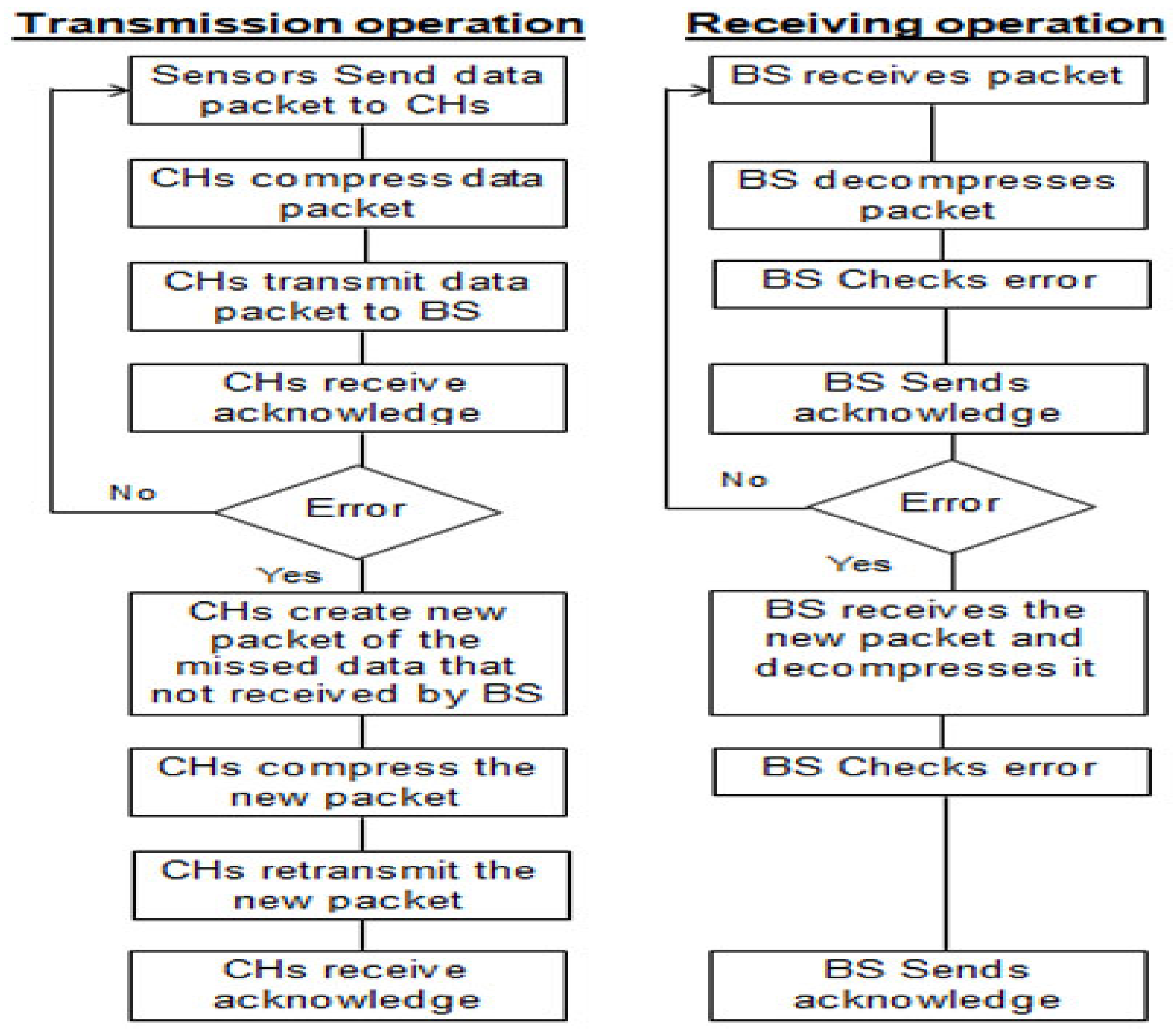
It is well known that transmission on wireless channels is much more error prone than on wired channels. Physical phenomena like reflection, diffraction, and scattering of waveforms, partially in conjunction with moving nodes or movements in the environment, lead to fast fading and inter-symbol interference. Path loss, attenuation, and the presence of obstacles lead to slow fading. In addition, there are noise and interference from other nodes/systems working in overlapping or neighboring frequency bands. Thus, transmission errors are inherent in wireless communications because of these instability of wireless channels, which is due to many reasons, for example, channel fading, time-frequency coherence, and inter-band interference [37]. To overcome the problem of recovery of transmitted data packet in case of error, we propose to resend the corrupted portion of the packet as illustrated in Figure 4.

Figure 4. Data communication in case of error.

Figure 4. Data communication in case of error.

4. Simulation Results

In this section, we evaluate the performance of the proposed protocol using MATLAB in terms of lifetime, throughput and stability of the network. The simultated WSN is composed of heterogeneous sensor nodes with different energy levels and transmission ranges.

4.1. Performance Metrics and Simulation Environment

In our simulation, we used the following metrics to validate the performance of the proposed EDACP-CS protocol:

• Energy consumption: Is measured by the total number of the network energy dissipation.
• Network lifetime: Is the time interval from the start of operation (of the sensor network) until the death of the last alive node.
• Throughput: Is the rate of data sent from the CHs to the BS over the network lifetime, measured per round per epoch.
• Stability period: Is the time interval from the start of network operation until the death of the first alive node. We call this period as stable region or period.
• Number of clusters: Indicates the number of clusters generated per round.

The simulation parameters are summarized in the following (Table 1).

Figure 5a shows the network topology comprised of 100 nodes corresponds to DWT basis. The networked data shown in Figure 5b can be presented with $K=10$ nonzero coefficients after DWT transform. Note: The locations of nodes are generated as random values drawn from the standard uniform distribution on the open interval (0, 100).

Table 1. Simulation Parameters.

Description	Parameter	Value
Number of nodes	N	100
Transmission ranges	$r_p$	$10,\dots ,80m$
Proportion of advanced nodes	m	0.2
Proportion of super nodes among advanced nodes	$m_0$	0.3
Energy factor for advanced nodes	α	3
Energy factor for super nodes	β	1.5
Initial energy level of normal nodes	$E_0$	0.5 J
Location of the BS	BS	(50, 50)
Data packet size	L	4000 bits
Network area	$R\times R$	$100\times 100m^2$
Radio Electronics Energy	$E_{elec}$	$50nJ/bit$
Transmit amplifier if $d_{BS}\le d_0$	${\mathrm{ϵ}}_{fs}$	$10pJ/(bit\ast m^2)$
Transmit amplifier if $d_{BS}\ge d_0$	${\mathrm{ϵ}}_{mp}$	$0.0013pJ/(bit\ast m^4)$
Threshold distance for swapping amplification model	$d_0$	$87.7058m$
Number of nonzero coefficients	K	10
Number of measurements	M	20

Table 1. Simulation Parameters.

Description	Parameter	Value
Number of nodes	N	100
Transmission ranges	$r_p$	$10,\dots ,80m$
Proportion of advanced nodes	m	0.2
Proportion of super nodes among advanced nodes	$m_0$	0.3
Energy factor for advanced nodes	α	3
Energy factor for super nodes	β	1.5
Initial energy level of normal nodes	$E_0$	0.5 J
Location of the BS	BS	(50, 50)
Data packet size	L	4000 bits
Network area	$R\times R$	$100\times 100m^2$
Radio Electronics Energy	$E_{elec}$	$50nJ/bit$
Transmit amplifier if $d_{BS}\le d_0$	${\mathrm{ϵ}}_{fs}$	$10pJ/(bit\ast m^2)$
Transmit amplifier if $d_{BS}\ge d_0$	${\mathrm{ϵ}}_{mp}$	$0.0013pJ/(bit\ast m^4)$
Threshold distance for swapping amplification model	$d_0$	$87.7058m$
Number of nonzero coefficients	K	10
Number of measurements	M	20

Figure 5. Sparsity of networked data in a Distributed Wavelet Transform (DWT) basis.

Figure 5. Sparsity of networked data in a Distributed Wavelet Transform (DWT) basis.

4.2. Experimental Results

The evaluation of performance metrics demonstrates the improvement and strength features of our design protocol compared with CS data collection, EECDA and LEACH-Hetero protocols. Here, we present the obtained performance results by the simulation.

4.2.1. Energy Consumption

Since energy consumption is the core issue in WSNs, we discuses the impact of our protocol on energy consumption by comparing the performance of the proposed protocol with existing protocols.

Figure 6 illustrates the difference of the energy consumed per round for different number of nodes in the network and different error estimation range ε in the proposed, EECDA, and LEACH-Hetero protocols. It is noticed that the energy consumption increases as the number of nodes increases in all protocols and EECDA performance is better than the performence of LEACH-Hetero, whereas EECDA maintains efficiently the energy consumption of sensor nodes by involving them in a single-hop communication within a cluster. Our proposed protocol outperforms EECDA, and LEACH-Hetero protocols in reducing the energy consumption. The reason is ECADP-CS uses the weighted election probabilities and the distances of sensor nodes to the BS in electing CHs, therefore, the energy efficiency is enhanced. From these results, it can be seen that the effect of the error estimation is not high in our proposed protocol.

Figure 6. Average energy consumption during error occurrence in ECADP-CS, energy efficient clustering and data aggregation (EECDA), and Low-Energy Adaptive Clustering Hierarchy (LEACH)-Hetero protocols.

Figure 6. Average energy consumption during error occurrence in ECADP-CS, energy efficient clustering and data aggregation (EECDA), and Low-Energy Adaptive Clustering Hierarchy (LEACH)-Hetero protocols.

Figure 7 shows that ECADP-CS conserves lower energy comparing with CS data collection protocol. This is because in ECADP-CS all the sensor nodes organize themselves into clusters with one node elected as a CH according to their weighted election probabilities and their distance to the BS leading to reducing the energy consumption of sensor nodes.

4.2.2. Network Lifetime

The network lifetime is an important metric for evaluating the performance of WSNs. Here, we discuses the impact of our proposed protocol on network lifetime by comparing the result of our proposed protocol with existing protocols.

Figure 8 shows the percentage of nodes alive in the network in EDACP-CS, EECDA, and LEACH-Hetero. It is obvious that both the dead time of the first and the last nodes of the proposed protocol came after those of LEACH-Hetero and EECDA. Also, it shows that EECDA achieves better performance compared with LEACH-Hetero, whereas in LEACH-Hetero the CH elected based on the residual energy of the individual node calculation and the re-clustering scheme is adopted in each cluster of the WSNs. However, a path with a maximum sum of energy residual would be selected for data transmission in spite of the path with minimum energy would be selected in case of EECDA. The prolongation of the network lifetime in EDACP-CS because it efficiently compresses data using CS in addition to considering the distance from the BS and the residual energy for the CH selection while other protocols select the CH by considering only the residual energy.

Figure 7. Energy consumption for the wireless sensor networks (WSN).

Figure 7. Energy consumption for the wireless sensor networks (WSN).

Figure 8. Number of alive nodes over rounds.

Figure 8. Number of alive nodes over rounds.

Figure 9 shows the lifetime for heterogeneous sensor nodes in terms of energy and transmission range. It has been observed that when the transmission range increases there is a significant improvement in lifetime of the network, this is because extending the transmission range will increase the number of CHs within the BS’s transmission range. Therefore, it reduces the amount of aggregated data packets which are forwarded to the BS since CHs near the BS have higher burden to receive and forward data packets. It has been shown that EDACP-CS greatly prolongs the sensor network’s lifetime compared with LEACH-Hetero and EECDA, because in EDACP-CS, each sensor node independently elects itself as a CH depends on both the energy level of each sensor and distance between sensor to neighbor’s sensor and sensors to BS. Besides, EDACP-CS efficiently compresses data using CS.

Figure 9. Transmission range vs. lifetime.

Figure 9. Transmission range vs. lifetime.

4.2.3. Throughput

A high throughput is essential for an efficient system. Figure 10 shows the overall throughput in terms of number of messages received at the BS from CHs, which is significantly greater in EDACP-CS against LEACH-Hetero and EECDA protocols. The reason is that EDACP-CS has three types of nodes (normal, advanced, and super) and takes into consideration the distance from the BS, because nodes that are closer to the BS and has higher residual energy than the other nodes have more chances to be selected as CHs for current round. Therefore, the super nodes become CHs more than both the advanced and normal nodes. The advanced nodes take up the role of CH more frequently than the normal nodes. Moreover, using CS would optimize energy usage to reduce storage space and energy consumption. Consequently, EDACP-CS has better network monitoring quality.

Figure 10. Throughput of the network.

Figure 10. Throughput of the network.

4.2.4. Stability

The stability period is crucial for many applications where the feedback from the WSNs must be reliable.

Figure 11 shows the network stability in the presence of the heterogeneity in energy level and transmission range. The proposed protocol provides best characteristics compared with EECDA and LEACH-Hetero in terms of lifetime, throughput, and stability. The reason is that EDACP-CS efficiently compresses data, besides the excelent selection of a sensor node to become a CH. Therefore, EDACP-CS efficiently balance the energy consumption among sensor nodes and hence the stability period is enhanced which is the main requirement for the lifetime of the WSNs.

Figure 11. Network stability in EDACP-CS, EECDA, and LEACH-Hetero.

Figure 11. Network stability in EDACP-CS, EECDA, and LEACH-Hetero.

4.2.5. Number of Cluster Heads

In this section, we test the number of selected CHs in every round in EDACP-CS, EECDA, and LEACH-Hetero protocols. As shown in Figure 12, EECDA and LEACH-Hetero has more uncertainties in CHs selection than EDACP-CS. This means that EDACP-CS is an efficient CHs selection protocol helps in better and constant data rate transmission to BS.

Figure 12. Number of cluster heads per round in EDACP-CS, EECDA, and LEACH-Hetero.

Figure 12. Number of cluster heads per round in EDACP-CS, EECDA, and LEACH-Hetero.

5. Conclusions

In this paper, an effective data acquisition clustered protocol using compressive sensing for heterogeneous WSNs in terms of energy and transmission range is proposed (EDACP-CS). In EDACP-CS, each sensor node independently elects itself as a cluster head based on its residual energy and distance form the BS. CS measurements are obtained via cluster heads. Distributed Wavelet Transform (DWT) is used as the sparsifying matrix and $i.i.d$ Gaussian with zero mean and unit variance is used as the sampling matrix. The simulation results reveal that our method decreases the energy consumption and therefore, prolongs the network lifetime and the stability period compared with EECDA and LEACH-Hetero protocols.