An Integer Linear Programming Formulation for the Minimum Cardinality Segmentation Problem

Abstract

In this article, we investigate the Minimum Cardinality Segmentation Problem (MCSP), an $\mathcal{NP}$-hard combinatorial optimization problem arising in intensity-modulated radiation therapy. The problem consists in decomposing a given nonnegative integer matrix into a nonnegative integer linear combination of a minimum cardinality set of binary matrices satisfying the consecutive ones property. We show how to transform the MCSP into a combinatorial optimization problem on a weighted directed network and we exploit this result to develop an integer linear programming formulation to exactly solve it. Computational experiments show that the lower bounds obtained by the linear relaxation of the considered formulation improve upon those currently described in the literature and suggest, at the same time, new directions for the development of future exact solution approaches to the problem.

1. Introduction

Let $S=\left\{s_{ij}\right\}$ be a $m\times n$ binary matrix. We say that S is a segment if for each row $i=1,\dots ,m$, the following consecutive ones property holds [1]:

$$\begin{array}{c}\hfill \text{if}{s}_{ij}=s_{i{j}^{\prime }}=1\text{for}1\le j<j^{\prime }\le n\text{then}{s}_{ik}=1\forall j<k<j^{\prime }\end{array}$$

(1)

Given an $m\times n$ nonnegative integer matrix $A=\left\{a_{ij}\right\}$, the Minimum Cardinality Segmentation Problem (MCSP) consists in finding a decomposition $A={\sum }_{t=1}^K{u}_t{S}_t$ such that $u_t\in {\mathbb{Z}}_{+}$, $S_t$ is a segment, for all $t\in 1,\dots ,K$, and K is minimum.

For example, consider the following nonnegative integer matrix:

$$\begin{array}{c}\hfill A=\left(\begin{array}{cccccc}0& 1& 1& 1& 1& 0\\ 1& 1& 2& 2& 2& 1\\ 1& 2& 4& 4& 2& 0\\ 1& 1& 2& 2& 1& 0\\ 0& 1& 1& 0& 0& 0\end{array}\right)\end{array}$$

(2)

then a possible decomposition of A into segments is [2]:

$$\begin{array}{ccc}\hfill A& =& 2\left(\begin{array}{cccccc}0& 0& 0& 0& 0& 0\\ 0& 0& 0& 0& 0& 0\\ 0& 0& 1& 1& 1& 0\\ 0& 0& 0& 0& 0& 0\\ 0& 0& 0& 0& 0& 0\end{array}\right)+1\left(\begin{array}{cccccc}0& 1& 1& 1& 0& 0\\ 0& 0& 1& 1& 1& 0\\ 0& 1& 1& 1& 0& 0\\ 0& 0& 1& 1& 0& 0\\ 0& 0& 0& 0& 0& 0\end{array}\right)+1\left(\begin{array}{cccccc}0& 0& 0& 0& 1& 0\\ 1& 1& 1& 1& 1& 1\\ 1& 1& 1& 1& 0& 0\\ 1& 1& 1& 1& 1& 0\\ 0& 1& 1& 0& 0& 0\end{array}\right)\hfill \end{array}$$

(3)

The MCSP arises in intensity modulated radiation therapy, currently considered one of the most powerful tools to treat solid tumors (see [3,4,5,6,7]). In this application, the matrix A usually encodes the intensity of the particle beam that has to be emitted by a linear accelerator at each instant of a radiation therapy session (see Figure 1). As the linear accelerator can only emit, instant per instant, a particle beam having a fixed intensity value rather than those encoded in A, the intensity matrix has to be decomposed into a set of segments, each encoding those elementary quantities of radiation, in order to deliver entry per entry the requested amount of radiation (see [7] for further details).

The MCSP is known to be $\mathcal{NP}$-hard even if the matrix A has only one row [1] or one column [8]. It is worth noting that the two restrictions mainly differ from each other for the type of segments considered. Specifically, in the one row case the segments are binary vector rows satisfying the consecutive ones property; in the one column case segments are just binary column vectors.

The $\mathcal{NP}$-hardness of the MCSP has justified the development of exact and approximate solution approaches aiming at solving larger and larger instances of the problem. These approaches have been recently reviewed in [7,9,10], and we refer the interested reader to these articles for further information. Here, we just focus on the exact solution approaches for the MCSP.

The literature on the MCSP reports on a number of studies focused on a specific restriction of the problem characterized by having the highest entry value of the matrix A, denoted as ${∥A∥}_{max}=max\left\{a_{ij}\right\}$, bounded by a positive constant H. This assumption is generally exploited e.g., in [1,11,12,13] to develop pseudo-polynomial exact solution algorithms for the considered restriction. A recent survey of these algorithms can be found in [7]. Surprisingly enough, however, in the last decade only a limited number of exact solution approaches have been proposed in the literature for the general problem. These approaches are restricted to the pseudo-polynomial solution algorithm described in [14], the Constraint Programming (CP) approaches described in [9,15], and the Integer Linear Programming (ILP) approaches described in [16,17,18,19]. Specifically, the algorithm proposed in [14] is based on an iterative process that exploits the pseudo-polynomial solution algorithm of [13] to solve at each step an instance of the MCSP characterized by having ${\displaystyle 1\le {∥A∥}_{max}=max\left\{a_{ij}\right\}\le H}$. The author shows that the algorithm is able to solve an instance of the general problem with an overal computational complexity $O({\left(mn\right)}^{2H+3})$. However, as shown in the computational experiments performed in [9], the algorithm proves to be very slow in practice.

The CP approach described in [15] was not initially conceived to solve the MCSP. In fact, the authors consider an objective function that minimizes at the same time a linear weighted combination of the number of segments involved in the decomposition and the sum of the coefficients used in the decomposition. As shown in [10], this approach can be adapted to solve the MCSP. However, the performances (in terms of solution times) so obtained are poorer than those relative to the CP approach described in [9]. Specifically, the authors of [9] first use an heuristic to find an initial feasible solution to the problem. Then, they attempt to find either a solution that uses less segments or to prove that the current solution is optimal. The certificate of optimality of the proposed algorithm is based on the use of an exhaustive search on the space of segments and coefficients compatible with the decomposition. As far as we are aware, this approach currently constitutes the fastest exact solution algorithm for the MCSP.

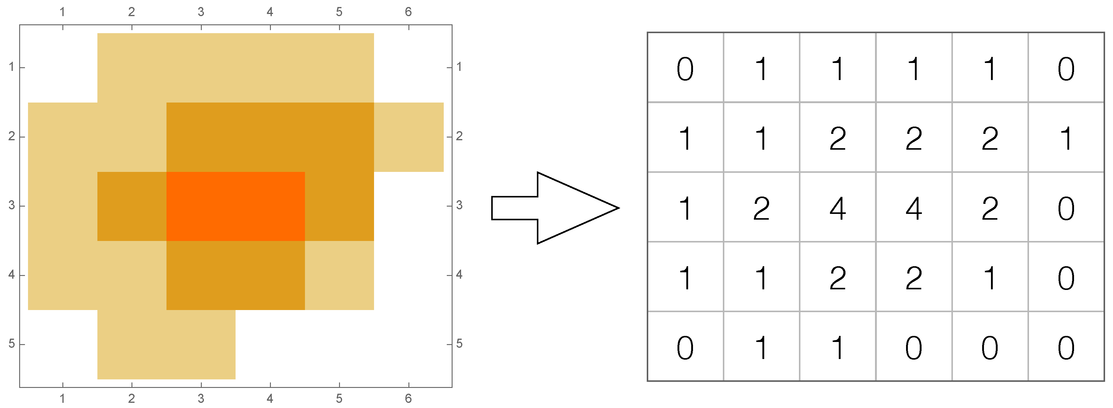
Figure 1. An example of discretization of the particle beam emitted by a linear accelerator (from [2]). The matrix on the right encodes the discretized intensity values of the radiation field shown on the left.

Figure 1. An example of discretization of the particle beam emitted by a linear accelerator (from [2]). The matrix on the right encodes the discretized intensity values of the radiation field shown on the left.

The ILP formulations described in the literature are usually characterized by worse performances than the constraint programming approach presented in [9]. The earliest ILP formulation was presented in [16] and is characterized by a polynomial number of variables and constraints. Specifically, provided an upper bound on the overall number of segments is used, the authors introduce a variable for each entry of each segment in the decomposition of the matrix A. This choice gives rise to multiple drawbacks: it may lead to very large formulations, it does not cut out the numerous equivalent (symmetric) solutions to the problem, and it is characterized by very poor performances in terms of solution times and size of the instances of the MCSP that can be analyzed [9,10]. The mixed integer linear programming formulation presented in [19] arises from an adaptation of the formulation used for a version Cutting Stock Problem [10]. As for [16], the formulation contains a polynomial number of variables and constraints and requires an upper bound on the overall number of segments used. As shown in [10], the formulation is characterized by better performances than the one presented in [16]. However, it proves unable to solve instances of the MCSP containing more than seven rows and seven columns. The polynomial-sized formulation presented in [18] has a strength point the fact that does not explicitly attempt at reconstructing the segments of the decomposition. This fact allows for both the reduction of the number of involved variables and a break in the symmetry introduced by the search of equivalent sets of segments. However, computational experiments carried out in [10] have shown that the linear relaxation of this formulation is usually very poor. This fact in turn leads to very long solution times [10]. A similar idea was used in [17]. In particular, the proposed polynomial-sized formulation minimizes the number of segments required in the decomposition of the matrix A, without explicitly computing them. This last step is possible in a subsequent moment via a post-processing of the optimal solution. However, also in this case, the formulation is characterized by poor computational performances when compared to the constraint programming approach described in [9], mainly due to the poor lower bounds provided by the linear relaxation.

Starting from the results described in C. Engelbeen’s Ph.D. thesis [20], in this article we investigate the problem of providing tighter lower bounds to the MCSP. Specifically, by using some results related to the one row restriction of the MCSP (see [2,20]), we transform the MCSP into a combinatorial optimization problem on a particular class of directed weighted networks and we present an exponential-sized ILP formulation to exactly solve it. Computational experiments show that the performances (in terms of solution times) of the formulation are still far from the CP approach described in [9]. However, the lower bounds obtained by the linear relaxation of the considered formulation generally improve upon those currently described in the literature. Thus, the theoretical and computational results discussed in this article may suggest new directions for the development of future exact solution approaches to the problem.

The article is organized as follows. After introducing some notation and definitions, in Section 2 we investigate the one row restriction of the MCSP. In particular, we transform the restriction into a combinatorial optimization problem on a weighted directed network and we investigate the optimality conditions that correlate both problems. In Section 3, we show how to generalize this transformation for generic intensity matrices and in Section 4 we present an ILP formulation for the MCSP based on this transformation. Finally, in Section 5 we present the computational results of the formulation, by providing some perspectives on future exact solution approaches to the problem.

2. The One Row Restriction of the MCSP as a Network Optimization Problem

In this section, we consider a restriction of the MCSP to the case in which the matrix A is a row vector. By following an approach similar to [15,20], we transform this restriction into a combinatorial optimization problem consisting of finding a shortest path in a particular weighted directed network. The insights provided by this transformation will prove useful both to extend the transformation to general matrices and to develop an ILP formulation for the general case of the MCSP. Before proceeding, we first introduce some notation and definitions similar to those already used in [2,9,20] and that will prove useful throughout the article.

Let q be a positive integer. We define a partition of q as a possible way of writing it as a sum of positive integers, i.e.,

$$\begin{array}{c}\hfill q=\sum _{j=1}^r{\beta }_j\end{array}$$

(4)

for some $r,{\beta }_j\in {\mathbb{Z}}_{+}$ (see [21]). For example, if we consider $q=4$ and we set $r=3$ and ${\beta }_1={\beta }_2=1$ and ${\beta }_3=2$ then a possible partition of 4 is $1+1+2$. We call Equation (4) the extended form of this particular partition of q. Interestingly, we also observe that an alternative way to partition q consists in writing it as a nonnegative integer linear combination of nonnegative integers, i.e.,

$$\begin{array}{c}\hfill q=\sum _{j=1}^s{\gamma }_j{\beta }_j\end{array}$$

(5)

for some $s,{\beta }_j,{\gamma }_j\in {\mathbb{Z}}_{+}$. For example, if we set $s=2$, ${\beta }_1=1$, ${\beta }_2=2$, ${\gamma }_1=2$, ${\gamma }_2=1$, then an alternative way to encode the considered partition is $(2·1)+(1·2)$. We call Equation (5) the compact form of this particular partition of q. The definition of a partition of a positive integer proves useful to investigate the one row restriction of the MCSP. In particular, it is worth noting that any decomposition of a row vector A into a sum of positive integers implicitly implies partitioning the entries of A. Then, a possible approach to solve the considered restriction consists in finding from among all of the possible partitions of each entry of A the ones that, appropriately combined, lead to the searched optimal decomposition.

To this end, we denote $H={\left|\right|A\left|\right|}_{max}=\max \left\{a_{ij}\right\}$, $\left[K\right]$ as the set $\{1,\dots ,K\}$, for some positive integer K, and we associate to the row vector A a particular weighted directed network $D=(V,\mathcal{A})$, called partition network, built as follows. Given an entry $a_j$ of A and a generic partition of $a_j$, let $q_w$ be the number of terms equal to w in the extended form of the considered partition or, equivalently, the coefficient associated to the term w in its compact form. Let V be the set of vertices including a source vertex s, a sink vertex t and a vertex for each partition of each entry of A:

$$\begin{array}{cccc}\hfill V& :=& \left\{s\right\}\cup \left\{t\right\}\hfill & \hspace{1em}\hspace{1em}\hspace{1em}\hspace{1em}\hspace{1em}\hspace{1em}\hspace{1em}\end{array}$$

(6)

$$\begin{array}{ccc}\hfill \hspace{1em}\hspace{1em}\hspace{1em}\hspace{1em}\hspace{1em} & & \cup \left\{(j;q_1,\dots ,q_H):\forall j\in \left[n\right],\forall (q_1,\dots ,q_H)\in {\mathbb{Z}}_{+}^H\text{s.t.}\sum _{w=1}^H{q}_w·w=a_j\right\}\hfill \end{array}$$

(7)

Let $\mathcal{A}$ be the set of arcs of D defined as follows:

$$\begin{array}{ccc}\hfill \mathcal{A}& :=& \{(s,(1;q_1,\dots ,q_H)):(1;q_1,\dots ,q_H)\in V\}\hfill \end{array}$$

(8)

$$\begin{array}{ccc}\hfill \hspace{1em}\hspace{1em} & & \cup \left\{((j;q_1,\dots ,q_H),(j+1;q_1^{\prime },\dots ,q_H^{\prime })):j\in [n-1]\right.\hfill \end{array}$$

(9)

$$\begin{array}{ccc}\hfill \hfill & & \left.(j;q_1,\dots ,q_H),(j+1;q_1^{\prime },\dots ,q_H^{\prime })\in V\right\}\hfill \end{array}$$

(10)

$$\begin{array}{ccc}\hfill & & \cup \{((n;q_1,\dots ,q_H),t):(n;q_1,\dots ,q_H)\in V\}\hfill \end{array}$$

(11)

Note that the construction of the partition network D is such that a decomposition of A corresponds to a path from the source to the sink in D. In particular, traversing a vertex $(j,q_1,\dots ,q_H)$ means that in the decomposition there are exactly $q_w$ segments with a coefficient equal to w and a 1 in position j, for all $w\in \left[H\right]$. Traversing an arc $((j;q_1,\dots ,q_H),(j+1;q_1^{\prime },\dots ,q_H^{\prime }))$ in the network means that in the corresponding decomposition of A there are exactly $q_w$ segments with a coefficient equal to w and a 1 in position j and exactly $q_w^{\prime }$ segments with a coefficient equal to w and a 1 in position $j+1$, for all $w\in \left[H\right]$. 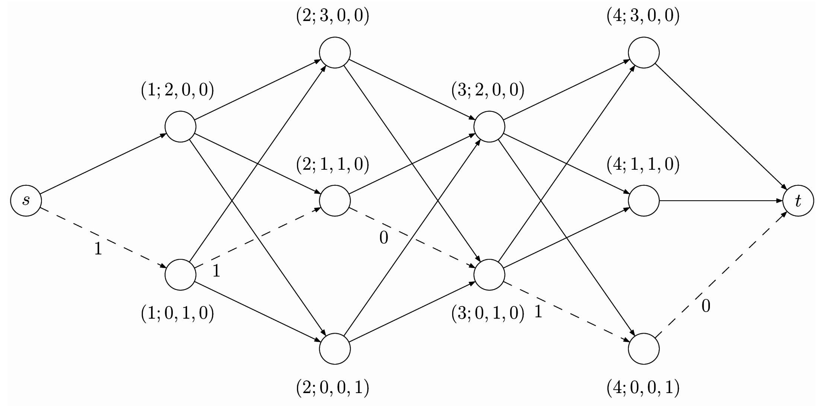As an example, Figure 2 shows the network corresponding to the row vector

$$\begin{array}{c}\hfill A=\left(\begin{array}{cccc}2& 3& 2& 3\end{array}\right)\end{array}$$

(12)

Figure 2. The partition network corresponding to the row $(2;3,2,3)$ with some lengths on arcs. The first two vertices on the right of s correspond to the two possible partitions of 2 (i.e., $2=1+1$ and $2=2$). The subsequent three vertices on the right correspond to the three possible partitions of 3 (i.e., $3=1+1+1$, $3=1+2$, $3=3$), and so on. Note that the entries of two subsequent columns, say j and $j+1$, in the row vector A induce a bipartite subnetwork in D. The dotted arcs represent the shortest $s-t$ path in D.

Figure 2. The partition network corresponding to the row $(2;3,2,3)$ with some lengths on arcs. The first two vertices on the right of s correspond to the two possible partitions of 2 (i.e., $2=1+1$ and $2=2$). The subsequent three vertices on the right correspond to the three possible partitions of 3 (i.e., $3=1+1+1$, $3=1+2$, $3=3$), and so on. Note that the entries of two subsequent columns, say j and $j+1$, in the row vector A induce a bipartite subnetwork in D. The dotted arcs represent the shortest $s-t$ path in D.

It is worth noting that, as we want to minimize the number of segments in the decomposition, whenever we cross arc $\left((j;q_1,\dots ,q_H),(j+1;q_1^{\prime },\dots ,q_H^{\prime })\right)$ we use $\max \{0,q_w-q_w^{\prime }\}$ segments with a coefficient equal to w, a 1 in position j and a zero in position $j+1$; $\min \{q_w,q_w^{\prime }\}$ segments with a coefficient equal to w and a 1 in both positions j and $j+1$ and finally $\max \{0,q_w^{\prime }-q_w\}$ segments with a coefficient equal to w, a zero in position j and a 1 in position $j+1$. Hence, passing from the vertex $(j;q_1,\dots ,q_H)$ to the vertex $(j+1;q_1^{\prime },\dots ,q_H^{\prime })$ implies to add $\max \{0,q_w^{\prime }-q_w\}$ new segments with a coefficient equal to w. In the light of these observations, consider a length function $\ell :\mathcal{A}⟶{\mathbb{Z}}_{+}$ defined as follows:

$$\begin{gathered} \ell \left(\alpha \right)=\left\{\begin{array}{cc}{\displaystyle \sum _{w=1}^H{q}_w}\hfill & \text{if}\alpha =(s,(1;q_1,\dots ,q_H)),(1;q_1,\dots ,q_H)\in V\hfill \\ {\displaystyle \sum _{w=1}^H\max \{0,q_w^{\prime }-q_w\}}\hfill & \mathrm{if}\alpha =((j;q_1,\dots ,q_H),(j+1;q_1^{\prime },\dots ,q_H^{\prime })) \\ ((j;q_1,\dots ,q_H),(j+1;q_1^{\prime },\dots ,q_H^{\prime }))\in \mathcal{A}\hfill \\ 0\hfill & \text{if}\alpha =((n;q_1,\dots ,q_H),t)\hfill \end{array}\right. \end{gathered}$$

(13)

Then, finding a decomposition of the row vector A into the minimum number of segments is equivalent to compute the length of any shortest $s-t$ path, denoted as $p_{st}$, in the corresponding weighted directed network D. Note that, due to the particular structure of the partition network D, such a problem is fixed-parameter tractable in H [2,20,22]. Once computed $p_{st}$, we can build the segments and the corresponding coefficients involved in the decomposition by iteratively applying the following approach. For all integers ℓ and r such that $\ell <r$, let $[\ell ,r)=\{\ell ,\ell +1,\dots ,r-1\}$. Set

$$\begin{array}{cccc}\hfill \ell & :=& \min \{j:q_w>0in(j;q_1,\dots ,q_H)\in p_{st}\}\hfill & \end{array}$$

(14)

$$\begin{array}{ccc}\hfill r& :=& \min \{j^{\prime }>\ell :q_w^{\prime }=0in(j^{\prime };q_1^{\prime },\dots ,q_H^{\prime })\in p_{st}\}.\hfill \end{array}$$

(15)

and build a segment S having the generic entry $s_j$ equal to 1 if $j\in [\ell ,r)$ and 0 otherwise. Associate to S a coefficient equal to w. Remove one unit in component $q_w$ from each vertex of the path that corresponds to an entry $j\in [\ell ,r)$ and iterate the procedure. As an example, the application of this procedure to the row vector Equation (12) leads to the following optimal solution:

$$A:=2\left(\begin{array}{cccc}1& 1& 1& 0\end{array}\right)+\left(\begin{array}{cccc}0& 1& 0& 0\end{array}\right)+3\left(\begin{array}{cccc}0& 0& 0& 1\end{array}\right)$$

In the next section, we show how to generalize this transformation to generic intensity matrices. This transformation will prove useful to develop an ILP formulation for the general version of the problem.

3. The MCSP as a Network Optimization Problem

Let A be a generic $m\times n$ nonnegative integer matrix. For each row $i\in \left[m\right]$ we build a partition network $D_i=\left(V_i,{\mathcal{A}}_i\right)$ in a way similar to the procedure described in Section 2. Specifically, for each row $i\in \left[m\right]$, the set $V_i$ includes a source vertex $s_i$ and a vertex for each partition of each entry of the i-th row of A:

$$\begin{array}{cccc}\hfill V_i& :=& \left\{s_i\right\}\hfill & \hspace{1em}\hspace{1em}\hspace{1em}\hspace{1em} \end{array}$$

(16)

$$\begin{array}{cc}\hspace{1em}\hspace{1em}\hspace{1em}\hspace{1em}\hspace{1em}\hspace{1em}\hspace{1em}\hspace{1em} & \cup \{\left(i,j;q_1,\dots ,q_H\right):j\in \left[n\right],\left(q_1,\dots ,q_H\right)\in {\mathbb{Z}}_{+}^H:\sum _{w=1}^H{q}_w·w=a_{ij}\}\hfill \end{array}$$

(17)

Similarly, the set ${\mathcal{A}}_i$ includes an arc for each pair of vertices corresponding to consecutive entries on the same row:

$$\begin{array}{ccc}\hfill {\mathcal{A}}_i& :=& \left\{\left(s_i,\left(i,1;q_1,\dots ,q_H\right)\right):\left(i,1;q_1,\dots ,q_H\right)\in V_i\right\}\hfill \end{array}$$

(18)

$$\begin{array}{cc}\hspace{1em}\hspace{1em}\hspace{1em}& \cup \left\{\left(\left(i,j;q_1,\dots ,q_H\right),\left(i,j+1;q_1^{\prime },\dots ,q_H^{\prime }\right)\right):j\in [n-1]\right.\hfill \end{array}$$

(19)

$$\begin{array}{cc}\hspace{1em}\hspace{1em}& \left.\left(i,j;q_1,\dots ,q_H\right),\left(i,j+1;q_1^{\prime },\dots ,q_H^{\prime }\right)\in V_i\right\}\hfill \end{array}$$

(20)

Consider the combined partition network $D=(V,\mathcal{A})$ having as vertexset

$$\begin{array}{c}\hfill V=\left\{s\right\}\cup \bigcup _{i\in \left[m\right]}{V}_i\cup \left\{t\right\}\end{array}$$

(21)

and as arcset

$$\begin{array}{c}\hfill \mathcal{A}=\{(s,s_i):i\in \left[m\right]\}\cup \bigcup _{i\in \left[m\right]}{\mathcal{A}}_i\cup \{\left(i,n;q_1,\dots ,q_H\right),t):i\in \left[m\right]\}\end{array}$$

(22)

D contains a vertex corresponding to each possible partition of each entry $a_{ij}$ of A. Each of these vertices is denoted by $\left(i,j;q_1,\dots ,q_H\right)$, where $\left(i,j\right)$ denotes the position of $a_{ij}$ in A, and $q_w$ denotes the number of terms equal to w in the extended form of the corresponding partition of $a_{ij}$ or, equivalently, the coefficient of w in its compact form, meaning $a_{ij}={\sum }_{w=1}^H{q}_w·w$. As an example, Figure 3 shows the combined partition network corresponding to the intensity matrix

$$\begin{array}{ccc}\hfill A& =& \left(\begin{array}{cc}2& 3\\ 3& 1\end{array}\right)\hfill \end{array}$$

(23)

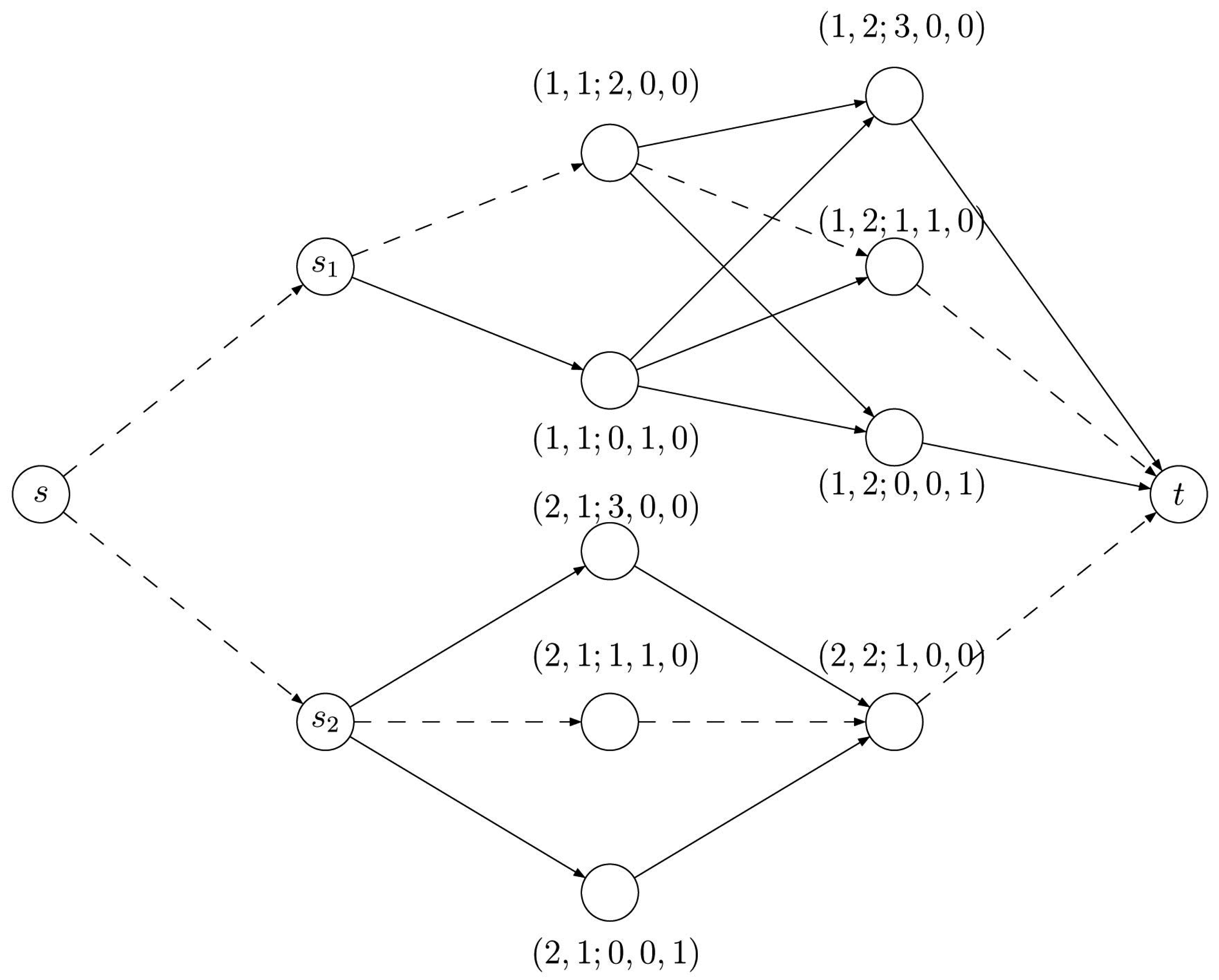
Figure 3. The combined partition network for matrix Equation (23). The dotted arcs represent a flow in the network that encodes a possible decomposition of A.

Figure 3. The combined partition network for matrix Equation (23). The dotted arcs represent a flow in the network that encodes a possible decomposition of A.

It is worth noting that, as for the one row restriction, a decomposition of the i-th row of A corresponds by construction to a path in the network $D_i$. In particular, traversing a vertex $(i,j;q_1,\dots ,q_H)$ means that in the decomposition, there are exactly $q_w$ matrices with a coefficient equal to w and a 1 in position $(i,j)$, for all $w\in \left[H\right]$.

Let $\ell :\mathcal{A}⟶{\mathbb{Z}}_{+}^H$ be a function that associate a H-dimensional length vector to each arc

$$\begin{array}{c}\hfill \alpha =\left(\left(i,j;q_1,\dots ,q_H\right),\left(i,j+1;q_1^{\prime },\dots ,q_H^{\prime }\right)\right)\in \mathcal{A}\end{array}$$

(24)

according to the following law:

$$\begin{gathered} \ell \left(\alpha \right)=\left\{\begin{array}{cc}\left(q_1,\dots ,q_H\right)\hfill & \text{if}\alpha =\left(s_i,\left(i,1;q_1,\dots ,q_H\right)\right),i\in \left[m\right]\hfill \\ \left(\max \left\{0,q_1^{\prime }-q_1\right\},\dots ,\max \left\{0,q_H^{\prime }-q_H\right\}\right)\hfill & \text{if}\alpha =\left(\left(i,j;q_1,\dots ,q_H\right),\left(i,j+1;q_1^{\prime },\dots ,q_H^{\prime }\right)\right) \\ i\in \left[m\right],j\in [n-1]\hfill \\ (0,\dots ,0)\hfill & \text{otherwise.}\hfill \end{array}\right. \end{gathered}$$

In particular, we use the convention to associate the length vector $(0,\dots ,0)$ to both the arcs leaving the source vertex s and the arcs entering the sink vertex t. For all the remaining arcs, the w-th entry of the length vector, denoted as ${\ell }_w\left(\alpha \right)$, represents the coefficient of w in the compact form of the corresponding partition of $a_{i,j+1}={\sum }_{w=1}^H{q}_w^{\prime }·w$ minus the coefficient of w in the compact form of the corresponding partition of $a_{ij}={\sum }_{w=1}^H{q}_w·w$, i.e., ${\ell }_w\left(\alpha \right):=\max \left\{0,q_w^{\prime }-q_w\right\}$. 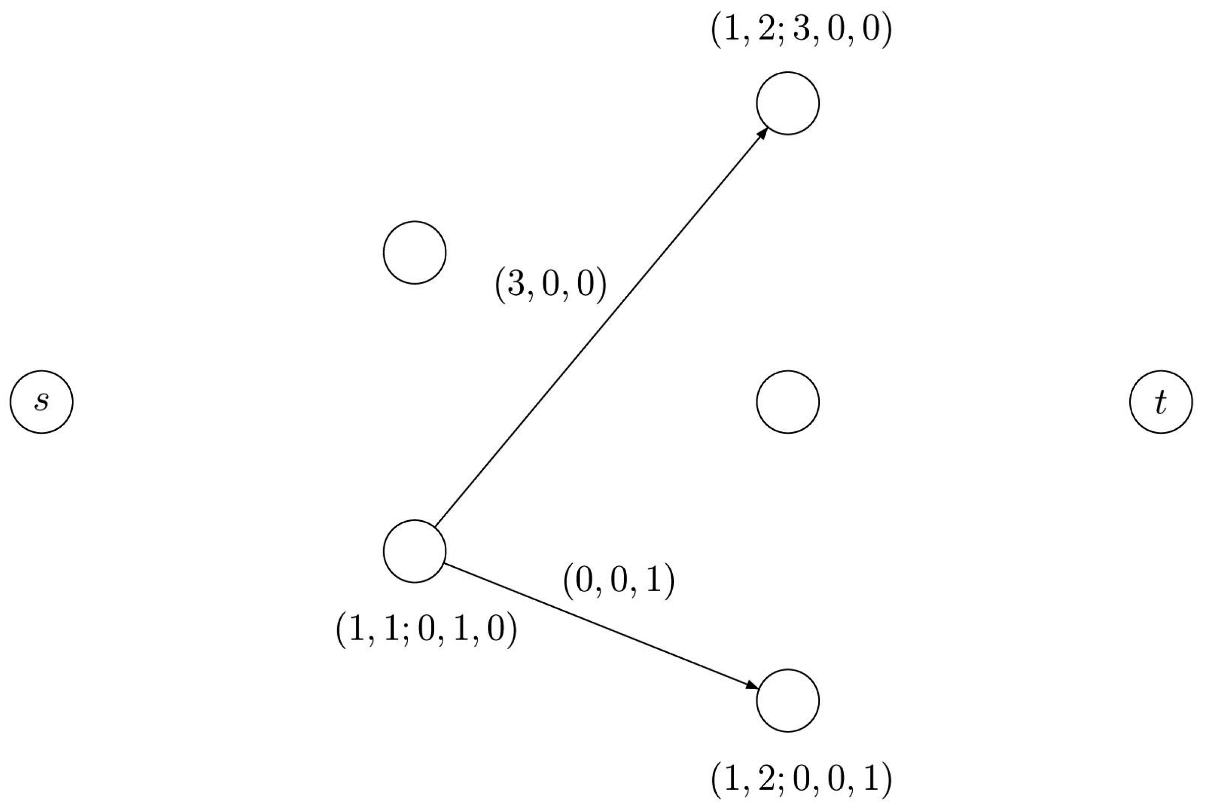As an example, Figure 4 provides the length vector of (certain arcs of) the partition network corresponding to the first row of matrix Equation (23), namely $\left(23\right)$.

Figure 4. The arc $\left(\right(1,1;0,1,0),(1,2;3,0,0\left)\right)$ represents a decomposition of the row vector $\left(23\right)$ in which entry 2 is decomposed by means of one segment having coefficient 2 and entry 3 is decomposed by means of three segments having coefficients 1. In order to move from partition $2=2$ to partition $3=1+1+1$, we need three new segments with a coefficient 1 and no segment with coefficient 2 or 3.

Figure 4. The arc $\left(\right(1,1;0,1,0),(1,2;3,0,0\left)\right)$ represents a decomposition of the row vector $\left(23\right)$ in which entry 2 is decomposed by means of one segment having coefficient 2 and entry 3 is decomposed by means of three segments having coefficients 1. In order to move from partition $2=2$ to partition $3=1+1+1$, we need three new segments with a coefficient 1 and no segment with coefficient 2 or 3.

It is easy to realize that any integral $s-t$ flow of value m in the combined partition network D associated to a given intensity matrix A, i.e., a $s-t$ flow in D composed by a family of $s_i-t$ flows, each lying in the subnetwork $D_i$, corresponds to a decomposition of the intensity matrix A. Any such flow is a combination of m paths $p_1,\dots ,p_m$ such that each $p_i$ is a $s-t$ path in the network $D_i$, for all $i\in \left[m\right]$. The length vector associated to this $s-t$ flow is

$$\begin{array}{c}\hfill \underset{i\in \left[m\right]}{\max }\left(\sum _{\alpha \in p_i}\ell \left(\alpha \right)\right):=\left(\underset{i\in \left[m\right]}{\max }\left\{\sum _{\alpha \in p_i}{\ell }_1\left(\alpha \right)\right\},\dots ,\underset{i\in \left[m\right]}{\max }\left\{\sum _{\alpha \in p_i}{\ell }_H\left(\alpha \right)\right\}\right)\end{array}$$

(25)

Note that the w-th component of vector Equation (25) provides the overall number of segments with a coefficient w in the decomposition of A. Hence, solving the MCSP is equivalent to find a $s-t$ flow of value m (that is, paths $p_1,\dots ,p_m$) such that the sum of all components of Equation (25) is minimized, or equivalently

$$\begin{array}{c}\hfill \min \sum _{w=1}^H\underset{i\in \left[m\right]}{\max }\left(\sum _{\alpha \in p_i}{\ell }_w\left(\alpha \right)\right)\end{array}$$

(26)

over all $s-t$ paths $p_1,\dots ,p_m$ in $D_1,\dots ,D_m$.

By referring to matrix Equation (23) and to the corresponding combined partition network shown in Figure 3, the length vector of the top-most dotted path $p_1$ equals $(2,0,0)+(0,1,0)=(2,1,0)$ and the length vector of the bottom-most dotted path $p_2$ equals $(1,1,0)$ + $(0,0,0)$ = $(1,1,0)$. The length vector of the whole flow equals $(2,1,0)$. Given paths $p_1$ and $p_2$, we can build the corresponding decomposition of the matrix A in the following way. For each component w, consider a nonnegative integer $m\times n$ matrix $A_w$ having the generic entry $(i,j)$ equal to the component $q_w$ in vertex $(i,j;q_1,\dots ,q_H)$ belonging to $p_i$. Then, the matrix A can be decomposed as

$$\begin{array}{c}\hfill A=\sum _{w=1}^{H}w·A_w\end{array}$$

(27)

As an example, by referring to the matrix Equation (23) and to the corresponding combined partition network shown in Figure 3, this procedure leads to the following decomposition of A:

$$\begin{array}{ccc}\hfill A& =& \left(\begin{array}{cc}2& 3\\ 3& 1\end{array}\right)=1\left(\begin{array}{cc}2& 1\\ 1& 1\end{array}\right)+2\left(\begin{array}{cc}0& 1\\ 1& 0\end{array}\right)\hfill \end{array}$$

(28)

It is worth noting that the matrices $A_w$ in general are not segments. However, it is possible to prove that each matrix $A_w$ can be in turn decomposed into a sum of segments, in such a way that the resulting decomposition is optimal for the MCSP. To this end, we introduce the following auxiliary problem:

The Beam-On Time Problem (BOTP). Given a nonnegative integer matrix A, find a decomposition $A={\sum }_{t=1}^K{u}_t{S}_t$ such that $u_t\in {\mathbb{Z}}_{+}$, $S_t$ is a segment, for all $t\in \left[K\right]$, and ${\sum }_{t=1}^K{u}_t$ is minimum.

The BOTP is polynomially solvable via the algorithms described in [1,20] and differs from the MCSP for the fact that it searches from among all the possible decompositions of the matrix A the one for which the sum of the coefficients is minimal.

Given a decomposition of A as in Equation (27), let us decompose $A_w$, for each $w\in \left[H\right]$, into a nonnegative integer linear combination of segments minimizing the BOTP. Then, Equation (27) can be rewritten as

$$\begin{array}{ccc}\hfill A& =& \sum _{w=1}^{H}w·A_w=\sum _{w=1}^{H}w·\left(\sum _{t:u_t=w}{S}_t\right)=\sum _{t=1}^K{u}_t{S}_t\hfill \end{array}$$

(29)

where $K={\sum }_{w=1}^H\left|\{t:u_t=w\}\right|$. The minimality of K in this new decomposition (i.e., the optimality of Equation (29) for the MCSP) is then proved by the following proposition:

Proposition 1. 

Let K be the optimal value to the MCSP. Then, the following equality holds:

$$K=\sum _{w=1}^{H}BOT\left(A_w\right)$$

where $BOT\left(A_w\right)$ denotes the minimum sum of ${\sum }_{t=1}^K{u}_t$ in the decomposition of $A_w$.

Proof. 

Let ${\beta }_w$ denote $\left|\left\{t:u_t=w\right\}\right|$, i.e., the sum of the coefficients in the decomposition of $A_w={\sum }_{t:u_t=w}{S}_t$, for all $w\in \left[H\right]$. Then, it holds that ${\beta }_w\ge BOT\left(A_w\right)$, for all $w\in \left[H\right]$. Hence, we have that

$$\begin{array}{c}\hfill K=\sum _{w=1}^H{\beta }_w\ge \sum _{w=1}^{H}BOT\left(A_w\right)\end{array}$$

(30)

To prove that in Equation (30) the strict equality holds, assume by contradiction that for some $\widehat{w}\in \left[H\right]$, ${\beta }_{\widehat{w}}>BOT\left(A_{\widehat{w}}\right)$. Then, it is possible to obtain a smaller value of ${\beta }_{\widehat{w}}$ by replacing ${\sum }_{t:u_t=\widehat{w}}{S}_t$ with the decomposition provided by the optimal solution of the BOTP with input $A_{\widehat{w}}$. However, ${\beta }_{\widehat{w}}$ is defined as the optimal solution to the BOTP with input $A_{\widehat{w}}$, hence this would contradict its optimality. Thus, the statement follows.  ☐

As an example, by using the decomposition algorithm for the BOTP described in [1,20] on the matrices $A_w$ in Equation (28), we obtain the following decomposition for Equation (23)

$$\begin{array}{c}\hfill A=\left(\begin{array}{cc}2& 3\\ 3& 1\end{array}\right)=1\left(\begin{array}{cc}2& 1\\ 1& 1\end{array}\right)+2\left(\begin{array}{cc}0& 1\\ 1& 0\end{array}\right)=\left(\begin{array}{cc}1& 0\\ 1& 1\end{array}\right)+\left(\begin{array}{cc}1& 1\\ 0& 0\end{array}\right)+2\left(\begin{array}{cc}0& 1\\ 1& 0\end{array}\right)\end{array}$$

(31)

which is optimal due to Proposition 1.

The transformation of the MCSP into a network optimization problem and the result provided by Proposition 1 constitute the fundation for the ILP formulation that will be presented in the next section.

4. An Integer Linear Programming Formulation for the MCSP

In this section, we develop an exponential-sized integer linear programming formulation for the MCSP. Unless not stated otherwise, throughout this section we will assume that A is a generic $m\times n$ nonnegative integer matrix.

Let $D=(V,\mathcal{A})$ be the combined partition network associated to A and let ${\mathcal{P}}_i$ be the set of all of the $s-t$ paths whose internal vertices belong to the subnetwork $D_i=(V_i,{\mathcal{A}}_i)$, for all $i\in \left[m\right]$. We associate to each path $p\in {\mathcal{P}}_i$, $i\in \left[m\right]$, a length vector $\ell \left(p\right)$ of dimension $H={\left|\right|A\left|\right|}_{\max }=\max \left\{a_{ij}\right\}$ obtained by summing over the lengths of the arcs belonging to p:

$$\begin{array}{c}\hfill \ell \left(p\right):=\sum _{\alpha \in p}\ell \left(\alpha \right)\end{array}$$

(32)

where $\left\{\ell \right(\alpha \left)\right\}$ are the length vectors defined in Section 3. Let ${\lambda }_p^i$ be a decision variable equal to 1 if path $p\in {\mathcal{P}}_i$, $i\in \left[m\right]$, is considered in the optimal solution to the problem and 0 otherwise. Finally, let $d_w$ be an integer variable equal to the number of segments with a coefficient w needed to decompose the matrix A. Then, a possible integer linear programming formulation for the MCSP is:

Formulation 1. 

– Integer Master Problem (IMP)

$$\begin{array}{}\mathrm{(33a)}& \hfill \min & \sum _{w=1}^H{d}_w\hfill & & \mathrm{(33b)}& \hfill s.t.& d_w\ge \sum _{p\in {\mathcal{P}}_i}{\ell }_w\left(p\right){\lambda }_p^i\hfill & \hfill & \forall i\in \left[m\right],\forall w\in \left[H\right]\hfill \mathrm{(33c)}& & \sum _{p\in {\mathcal{P}}_i}{\lambda }_p^i=1\hfill & \hfill & \forall i\in \left[m\right]\hfill \mathrm{(33d)}& & {\lambda }_p^i\in \{0,1\}\hfill & \hfill & \forall i\in \left[m\right],\forall p\in {\mathcal{P}}_i\hfill \mathrm{(33e)}& & d_w\in {\mathbb{Z}}_{+}\hfill & \hfill & \forall w\in \left[H\right]\hfill \end{array}$$

The objective function Equation (33a) accounts for the number of segments involved in the decomposition of the matrix A. Constraints Equation (33b) impose that for each row $i\in \left[m\right]$, the number of segments with coefficient w has to be greater than or equal to ${\max }_{i\in \left[m\right]}\{{\sum }_{\alpha \in p_i}{\ell }_w\left(\alpha \right)\}$, which corresponds to the w-th component of the length vector associated to the $s-t$ flow in D. Constraints Equation (33c) impose to choose exactly one path in each partition network $D_i$. Finally, constraints Equations (33d) and (33e) impose the integrality constraint on the considered variables. The validity of Formulation 1 is guaranteed by the transformation described in Section 3. It is worth noting that we need not to impose the integrality constraint on variables $d_w$. In fact, it is easy to see that in an optimal solution to IMP, the integrality of variables ${\lambda }_p^i$ together with Equation (33b) suffice to guarantee the integrality of variables $d_w$. Formulation 1 includes an exponential number of (path) variables and a number of constraints that grows pseudo-polynomially in function of H. A possible approach to solve it consists of using column generation and branch-and-price techniques [23].

In order to study the pricing oracle, consider the following formulation:

Formulation 2. 

– Restricted Linear Program Master (RLPM)

$$\begin{array}{}\mathrm{(34a)}& \hfill \min & \sum _{w=1}^H{d}_w\hfill & & \mathrm{(34b)}& \hfill s.t.& d_w\ge \sum _{p\in {\tilde{\mathcal{P}}}_i}{\ell }_w\left(p\right){\lambda }_p^i\hfill & \hfill & \forall i\in \left[m\right],\forall w\in \left[H\right]\hfill \mathrm{(34c)}& & \sum _{p\in {\tilde{\mathcal{P}}}_i}{\lambda }_p^i=1\hfill & \hfill & \forall i\in \left[m\right]\hfill \mathrm{(34d)}& & {\lambda }_p^i\ge 0\hfill & \hfill & \forall i\in \left[m\right],\forall p\in {\tilde{\mathcal{P}}}_i\hfill \mathrm{(34e)}& & d_w\ge 0\hfill & \hfill & \forall w\in \left[H\right]\hfill \end{array}$$

where ${\tilde{\mathcal{P}}}_i$ is a strict subset of ${\mathcal{P}}_i$, $i\in \left[m\right]$, and let ${\pi }_{i,w}$ and ${\mu }_i$ be the dual variables associated to constraints Equations (33b) and (33c), respectively. Then, the dual problem associated to the IMP is:

Formulation 3. 

– Dual Problem (DP)

$$\begin{array}{}\mathrm{(35a)}& \hfill \max & \sum _{i=1}^m{\mu }_i\hfill & & \mathrm{(35b)}& \hfill s.t.& {\mu }_i-\sum _{w=1}^H{\pi }_{i,w}{\ell }_w\left(p\right)\le 0\hfill & \hfill & \forall i\in \left[m\right],\forall p\in {\mathcal{P}}_i\hfill \mathrm{(35c)}& & \sum _{i=1}^m{\pi }_{i,w}=1\hfill & \hfill & \forall w\in \left[H\right]\hfill \mathrm{(35d)}& & {\pi }_{i,w}\ge 0\hfill & \hfill & \forall i\in \left[m\right],\forall w\in \left[H\right]\hfill \mathrm{(35e)}& & {\mu }_i\mathit{unrestricted}\hfill & \hfill & \forall i\in \left[m\right]\hfill \end{array}$$

A variable with negative reduced cost in the RLPM corresponds to a dual constraint violated by the current dual solution. As variables $d_w$ are always present in the RLPM, constraints Equation (35c) will never be violated. To check the existence of violated constraints, Equation (35b) means searching for the existence of a row $\widehat{i}\in \left[m\right]$ and a path $\widehat{p}\in {\mathcal{P}}_{\widehat{i}}$ such that

$$\begin{array}{c}\hfill {\mu }_{\widehat{i}}-\sum _{w=1}^H{\pi }_{\widehat{i},w}{\ell }_w\left(\widehat{p}\right)>0.\end{array}$$

(36)

Let ${\pi }_{i,w}^{*}$ and ${\mu }_i^{*}$ be the values of variables ${\pi }_{i,w}$ and ${\mu }_i$ in the current dual solution. Consider a new length function ${\ell }^{*}:{\mathcal{A}}_{\widehat{i}}⟶{\mathbb{R}}^{+}$ defined as

$$\begin{array}{c}\hfill {\ell }^{*}\left(\alpha \right):=\sum _{w=1}^H{\pi }_{i,w}^{*}{\ell }_w\left(\alpha \right)\end{array}$$

(37)

and let $D_{\widehat{i}}^{*}$ be the partition network $D_{\widehat{i}}$ with lengths provided by Equation (37). By definition, the length $\ell \left(p\right)$ of a $s-t$ path $p\in {\mathcal{P}}_i$ in D is equal to

$$\begin{array}{c}\hfill {\ell }^{*}\left(p\right):=\sum _{\alpha \in p}\sum _{w=1}^H{\pi }_{i,w}^{*}{\ell }_w\left(\alpha \right)=\sum _{w=1}^H{\pi }_{i,w}^{*}{\ell }_w\left(p\right).\end{array}$$

(38)

Then, determining the existence of a path violating Equation (35b) implies to check whether the shortest $s-t$ path in $D_{\widehat{i}}^{*}$ has an overall length shorter than ${\mu }_i^{*}$, i.e., to check if it holds that

$$\begin{array}{c}\hfill \sum _{w=1}^H{\pi }_{\widehat{i},w}^{*}{\ell }_w\left(\widehat{p}\right)<{\mu }_{\widehat{i}}^{*}.\end{array}$$

(39)

Since all length values are nonnegative, this task can be performed by using a standard implementation of Dijkstra’s algorithm [22].

5. Computational Experiments

In this section, we analyze the performance of Formulation 1 in solving instances of the MCSP. Our experiments were motivated by a twofold goal: to compare the lower bounds provided by the linear relaxation of Formulation 1 vs. the lower bounds provided by the linear relaxations of the ILP formulations described in [17,18,19]; and to measure the runtime performances of Formulation 1. We emphasize that our experiments neither attempt to investigate the use of Formulation 1 in IMRT nor to compare Formulation 1 to other algorithms that use an objective function that is different from the one used in the MCSP. The reader interested in a systematic discussion about such issues is referred to [7,10].

In order to measure the quality of the lower bounds provided by the linear relaxation of Formulation 1, we considered the instances of the MCSP provided in Chapter 2 of L. R. Mason’s Ph.D. thesis [10]. One of the advantage of considering Mason’s instances derives from the fact that the author first compared the linear relaxations of the ILP formulations described in [17,18,19], by creating benchmarks that can be used for further comparisons. The author considered a dataset constituted by 25 squared matrices having an order ranging in $\{6,\dots ,10\}$. Fixed an order, the dataset provides five random instances of the MCSP having $H={\left|\right|A\left|\right|}_{\max }\le 15$ if the order is smaller than or equal to eight, and $H={\left|\right|A\left|\right|}_{\max }=10$ otherwise. We refer the interested reader to Chapter 2 of [10] for further information concerning the performances of the considered ILP formulations and to the appendix of the same work to download the instances used in this work.

5.1. Implementing Formulation 1

One of the main difficulties in designing a solution approach for Formulation 1 consists of devising effective branching rules when the binary variables are priced out at run time. In particular, a typical problem is that there may be no easy way to forbid that a variable that was fixed at 0 by branching could still be a feasible solution for the pricing problem. However, if the value of H is relatively small, it is possible to overcome this issue by branching on “arc variables” rather than on “path variables”. Specifically, let us add in Formulation 1 a new decision (arc) variable $x_{\alpha }$ equal to 1 if arc $\alpha \in \mathcal{A}$ is used and 0 otherwise. Then, an alternative formulation for the MCSP is:

Formulation 4. 

– Path-Arc Integer Master Problem (PA-IMP)

$$\begin{array}{}\mathrm{(40a)}& \hfill \min & \sum _{w=1}^H{d}_w\hfill & & \mathrm{(40b)}& \hfill s.t.& d_w\ge \sum _{p\in {\mathcal{P}}_i}{\ell }_w\left(p\right){\lambda }_p^i\hfill & \hfill & \forall i\in \left[m\right],\forall w\in \left[H\right]\hfill \mathrm{(40c)}& & \sum _{p\in {\mathcal{P}}_i}{\lambda }_p^i=1\hfill & \hfill & \forall i\in \left[m\right]\hfill \mathrm{(40d)}& & \sum _{\begin{array}{c}p\in {\mathcal{P}}_i:\\ \alpha \in p\end{array}}{\lambda }_p^i\le x_{\alpha }\hfill & \hfill & \forall \alpha \in \left[{\mathcal{A}}_i\right],\forall i\in \left[m\right]\hfill \mathrm{(40e)}& & \sum _{\alpha \in {\mathcal{A}}_i}{x}_{\alpha }=n-1\hfill & \hfill & \forall i\in \left[m\right]\hfill \mathrm{(40f)}& & {\lambda }_p^i\in \{0,1\}\hfill & \hfill & \forall i\in \left[m\right],\forall p\in {\mathcal{P}}_i\hfill \mathrm{(40g)}& & x_{\alpha }\in \{0,1\}\hfill & \hfill & \forall \alpha \in \mathcal{A}\hfill \mathrm{(40h)}& & d_w\in {\mathbb{Z}}_{+}\hfill & \hfill & \forall w\in \left[H\right].\hfill \end{array}$$

In particular, Formulation 4 has the same constraints that Formulation 1 plus constraints Equation (40d) that impose that only selected arcs can be used in a path $p\in {\mathcal{P}}_i$, $i\in \left[m\right]$ and constraints Equation (40e) that impose that in each path in $D_i$ is made up of exactly $n-1$ arcs.

Proposition 2. 

In any feasible solution to Formulation 4, the integrality of variables $x_{\alpha }$ together with constraints Equations (40c) and (40d) suffice to guarantee the integrality of variables ${\lambda }_p^i$.

Proof. 

Assume by contradiction that there exists a feasible solution to the PA-IMP in which there are both a row $\tilde{i}\in \left[m\right]$ and a path $p_{\tilde{i}}$ such that $0<{\lambda }_{p_{\tilde{i}}}^{\tilde{i}}<1$. Then, due to constraint Equation (40c), there also exists at least another nonzero fractional path variable encoding an alternative path for row $\tilde{i}$. These two paths must differ for at least one arc. We denote ${\alpha }_1$ as the arc used by path ${\lambda }_{p_{\tilde{i}}}^{\tilde{i}}$ and ${\alpha }_2$ as the arc used by the other fractional variable. Because of constraint Equations (40d) and (40g), this fact implies that both variables $x_{{\alpha }_1}$ and $x_{{\alpha }_2}$ are equal to one, which implies that constraint Equation (40e) must be violated for $\tilde{i}$. This, in turn, contradicts the feasibility of the solution.  ☐

An immediate consequence of the above proposition is that

Proposition 3. 

The integrality constraint on variables ${\lambda }_p^i$ in Formulation 4 can be relaxed.

It is worth noting that the number of arcs in the combined partition network associated with the matrix A grows exponentially in function of H. Hence, we stress that the introduction of the arc variables is practical only for small values of H.

As for Formulation 1, the linear programming relaxation of Formulation 4, denoted as PA-RLMP, can be solved via column generation techniques [23]. To this end, we define the following dual variables associated to constraints Equations (40b)–(40e), namely ${\pi }_{i,w}$, for all $i\in \left[m\right]$ and $w\in \left[H\right]$; ${\mu }_i$, for all $i\in \left[m\right]$; ${\eta }_{i\alpha }$, for all $\alpha \in \left[{\mathcal{A}}_i\right]$, $i\in \left[m\right]$; and ${\omega }_i$, for all $i\in \left[m\right]$. The dual of the PA-RLMP has the following constraints:

$$\begin{array}{ccc}\hfill {\mu }_i-\sum _{w=1}^H\left(\sum _{\alpha \in p}{\ell }_w\left(\alpha \right)\right){\pi }_{iw}-\sum _{\alpha \in p}{\eta }_{i\alpha }\le 0& & \forall i\in \left[m\right],\forall p\in {\mathcal{P}}_i\hfill \end{array}$$

(41)

$$\begin{array}{ccc}\hfill \sum _{i=1}^m{\pi }_{i,w}=1& & \forall w\in \left[H\right]\hfill \end{array}$$

(42)

$$\begin{array}{ccc}\hfill {\eta }_{i\alpha }+{\omega }_i\le 0& & \forall i\in \left[m\right];\forall \alpha \in \left[{\mathcal{A}}_i\right]\hfill \end{array}$$

(43)

As variables $d_w$ are always present in the RLPM, constraints Equation (42) will never be violated in the current dual solution. Assuming that $\left|\mathcal{A}\right|$ arc variables are always present in the PA-RLMP, constraints Equation (43) will never be violated. To check the existence of violated constraints Equation (41) means searching for the existence of a row $\widehat{i}\in \left[m\right]$ and a path $\widehat{p}\in {\mathcal{P}}_{\widehat{i}}$ such that

$$\begin{array}{c}\hfill {\mu }_{\widehat{i}}-\sum _{w=1}^H\left(\sum _{\alpha \in \widehat{p}}{\ell }_w\left(\alpha \right)\right){\pi }_{\widehat{i}w}-\sum _{\alpha \in \widehat{p}}{\eta }_{\widehat{i}\alpha }>0\end{array}$$

(44)

It is easy to see that, by denoting ${\pi }_{i,w}^{*}$, ${\mu }_i^{*}$ and ${\eta }_{i\alpha }^{*}$ as the values of variables ${\pi }_{i,w}$, ${\mu }_i$ and ${\eta }_{i\alpha }$ in the current dual solution and by using argumentations similar to those used in Section 3, determining the existence of violated constraints Equation (41) is equivalent to check whether the shortest $s-t$ path in $D_{\widehat{i}}^{*}$ has an overall length shorter than ${\mu }_i^{*}-{\sum }_{\alpha \in \widehat{p}}{\eta }_{\widehat{i}\alpha }^{*}$, i.e., to check if it holds that

$$\begin{array}{c}\hfill \sum _{w=1}^H{\pi }_{\widehat{i},w}^{*}{\ell }_w\left(\widehat{p}\right)<{\mu }_{\widehat{i}}^{*}-\sum _{\alpha \in \widehat{p}}{\eta }_{\widehat{i}\alpha }^{*}\end{array}$$

(45)

Once again, this task can be performed by using a standard implementation of Dijkstra’s algorithm [22].

5.2. Implementation Details

We implemented Formulation 4 in FICO Xpress Mosel, version 3.8.0, Optimizer libraries v27.01.02 (64-bit, Hyper capacity). We run the algorithm on an IMac Core i7, 3.50 GHz, equipped with 16 GByte RAM and operating system Mac Os X, Darwin version 10.10.3, gcc version 4.2.1 (LLVM version 6.1.0, clang-602.0.53). We used the default settings for Fico Xpress Optimizer and we set 1 h as maximum runtime for each instance of the problem as in [9,10]. The source code of the algorithm can be downloaded from [24].

5.2.1. Primal Bound

We constructed the primal bound of the problem by solving the one row restriction of the MCSP for each row of the matrix A. This task can be performed in polynomial time by using the algorithm described in Section 2. We computed the length of the corresponding $s-t$ flow by using Equation (25) and set the value of this solution equal to the sum of the corresponding components.

5.2.2. Setting Initial Columns

We set the initial columns of the RLPM by choosing at random a path in $D_i$, for each $i\in \left[m\right]$. We solved the linear programming relaxation at each node of the search tree by implementing the pricing problem described in the previous section. In particular, we used a strategy similar to the one described in [25], i.e., we added to ${\tilde{P}}_i$, $i\in \left[m\right]$, all of the paths violating Equation (41).

5.2.3. Branching Rules

We explored the search tree by branching on the arc variables $x_{\alpha }$. In particular, we first constructed a $s-t$ flow in D. Subsequently, we used a depth-first approach in which we backtracked first on the arcs belonging to the partition network $D_m$; if the backtracking returns to $s_m$ then we backtracked on the arcs belonging to the partition network $D_{m-1}$ and subsequently we returned to those belonging to $D_m$. We recursively iterated this approach for all of the partition networks in D.

5.3. Performance Analysis

Table 1 shows the comparison between the linear relaxation of Formulation 4 and the linear relaxations of the formulations described in [17,18,19] when considering Mason’s instances. Some of the values presented in the table refer to the computational tests performed in Mason’s Ph.D. thesis (namely those reported in Tables 2.7 ad 2.8 of [10]). Specifically, the first column provides the name of the instances analyzed. The second column provides the corresponding optimal values. The third column provides the linear programming relaxations of the formulations described in [17,18,19], denoted as $M_C$, $M_W$, and $M_M$, respectively. The fourth column provides the values of the gap of formulations $M_C$, $M_W$, and $M_M$ expressed in percentage, i.e., the difference between the optimal value to a given instance of the MCSP and the objective function value of the linear programming relaxation at the root node of the respective search tree, divided by the optimal value. The fifth column provides the linear programming relaxations of the formulations $M_C$ and $M_M$ when considering the constraints (2.16) and (2.45) in Mason’s Ph.D. thesis (denoted as $M_C^{+}$ and $M_M^{+}$, respectively) and the sixth column provides the corresponding gaps. The seventh and the eighth columns provide the lower bounds and the gaps of the shortest path formulation [15] as modified in [10], hereafter denoted as “SR”. This formulation consider a relaxation of the MCSP obtained when partitioning the MCSP into a set of independent sub-problems, one for each row of the matrix A. Finally, the ninth column provides the linear programming relaxations of Formulation 4, the tenth column provides the corresponding gaps, and the eleventh column provides the gaps when ceiling the values of the corresponding linear relaxation of Formulation 4.

Table 1. Comparison of the linear relaxation of Formulation 4 vs. the linear relaxations of the formulations described in [15,17,18,19] when considering the instances of the minimum cardinality segmentation problem (MCSP) described in [10].

Instance	Optimum	LB	Gap (%)	LB	Gap (%)	LB	Gap (%)	LB	Gap (%)	Gap (%)
		$M_C,M_W,M_M$		$M_C^{+},M_M^{+}$		SR		F4		$⌈{\mathrm{LB}}_{F4}⌉$
p6-6-15-0	7	1.80	74.29	4.84	30.85	6.00	14.29	6.19	11.57	0.00
p6-6-15-1	7	1.87	73.33	4.78	31.78	6.00	14.29	6.34	9.43	0.00
p6-6-15-2	7	1.60	77.14	4.38	37.49	6.00	14.29	6.01	14.14	0.00
p6-6-15-3	7	1.67	76.19	4.37	37.55	6.00	14.29	6.13	12.43	0.00
p6-6-15-4	8	2.53	68.33	5.53	30.82	6.00	25.00	6.84	14.50	12.50
p7-7-15-0	8	2.27	71.67	5.41	32.32	7.00	12.50	7.70	3.75	0.00
p7-7-15-1	8	2.60	67.50	5.51	31.09	7.00	12.50	7.11	11.13	0.00
p7-7-15-2	8	1.87	76.67	5.03	37.08	7.00	12.50	7.00	12.50	12.50
p7-7-15-3	9	2.40	73.33	5.94	34.01	7.00	22.22	7.70	14.44	11.11
p7-7-15-4	8	1.67	79.17	4.42	44.70	6.00	25.00	6.89	13.88	12.50
p8-8-15-0	9	2.53	71.85	6.13	31.90	7.00	22.22	8.13	9.67	0.00
p8-8-15-1	8	2.33	70.83	5.51	31.07	7.00	12.50	7.52	6.00	0.00
p8-8-15-2	9	2.13	76.30	5.81	35.50	8.00	11.11	8.06	10.44	0.00
p8-8-15-3	9	2.13	76.30	5.61	37.66	8.00	11.11	8.07	10.33	0.00
p8-8-15-4	9	2.40	73.33	6.04	32.90	8.00	11.11	8.00	11.11	11.11
p9-9-10-0	9	2.60	71.11	6.45	28.32	8.00	11.11	8.50	5.56	0.00
p9-9-10-1	8	2.50	68.75	5.65	29.34	8.00	0.00	8.00	0.00	0.00
p9-9-10-2	8	2.20	72.50	5.40	32.48	7.00	12.50	7.68	4.00	0.00
p9-9-10-3	9	2.30	74.44	5.80	35.53	8.00	11.11	8.14	9.56	0.00
p9-9-10-4	9	2.80	68.89	5.96	33.83	8.00	11.11	8.58	4.67	0.00
p10-10-10-0	10	2.90	71.00	6.55	34.50	9.00	10.00	9.00	10.00	10.00
p10-10-10-1	10	3.10	69.00	7.22	27.84	9.00	10.00	9.00	10.00	10.00
p10-10-10-2	10	3.70	63.00	7.28	27.25	9.00	10.00	9.50	5.00	0.00
p10-10-10-3	10	3.60	64.00	8.15	18.52	9.00	10.00	9.35	6.50	0.00
p10-10-10-4	10	3.40	66.00	7.29	27.13	9.00	10.00	9.18	8.20	0.00

Table 1. Comparison of the linear relaxation of Formulation 4 vs. the linear relaxations of the formulations described in [15,17,18,19] when considering the instances of the minimum cardinality segmentation problem (MCSP) described in [10].

Instance	Optimum	LB	Gap (%)	LB	Gap (%)	LB	Gap (%)	LB	Gap (%)	Gap (%)
		$M_C,M_W,M_M$		$M_C^{+},M_M^{+}$		SR		F4		$⌈{\mathrm{LB}}_{F4}⌉$
p6-6-15-0	7	1.80	74.29	4.84	30.85	6.00	14.29	6.19	11.57	0.00
p6-6-15-1	7	1.87	73.33	4.78	31.78	6.00	14.29	6.34	9.43	0.00
p6-6-15-2	7	1.60	77.14	4.38	37.49	6.00	14.29	6.01	14.14	0.00
p6-6-15-3	7	1.67	76.19	4.37	37.55	6.00	14.29	6.13	12.43	0.00
p6-6-15-4	8	2.53	68.33	5.53	30.82	6.00	25.00	6.84	14.50	12.50
p7-7-15-0	8	2.27	71.67	5.41	32.32	7.00	12.50	7.70	3.75	0.00
p7-7-15-1	8	2.60	67.50	5.51	31.09	7.00	12.50	7.11	11.13	0.00
p7-7-15-2	8	1.87	76.67	5.03	37.08	7.00	12.50	7.00	12.50	12.50
p7-7-15-3	9	2.40	73.33	5.94	34.01	7.00	22.22	7.70	14.44	11.11
p7-7-15-4	8	1.67	79.17	4.42	44.70	6.00	25.00	6.89	13.88	12.50
p8-8-15-0	9	2.53	71.85	6.13	31.90	7.00	22.22	8.13	9.67	0.00
p8-8-15-1	8	2.33	70.83	5.51	31.07	7.00	12.50	7.52	6.00	0.00
p8-8-15-2	9	2.13	76.30	5.81	35.50	8.00	11.11	8.06	10.44	0.00
p8-8-15-3	9	2.13	76.30	5.61	37.66	8.00	11.11	8.07	10.33	0.00
p8-8-15-4	9	2.40	73.33	6.04	32.90	8.00	11.11	8.00	11.11	11.11
p9-9-10-0	9	2.60	71.11	6.45	28.32	8.00	11.11	8.50	5.56	0.00
p9-9-10-1	8	2.50	68.75	5.65	29.34	8.00	0.00	8.00	0.00	0.00
p9-9-10-2	8	2.20	72.50	5.40	32.48	7.00	12.50	7.68	4.00	0.00
p9-9-10-3	9	2.30	74.44	5.80	35.53	8.00	11.11	8.14	9.56	0.00
p9-9-10-4	9	2.80	68.89	5.96	33.83	8.00	11.11	8.58	4.67	0.00
p10-10-10-0	10	2.90	71.00	6.55	34.50	9.00	10.00	9.00	10.00	10.00
p10-10-10-1	10	3.10	69.00	7.22	27.84	9.00	10.00	9.00	10.00	10.00
p10-10-10-2	10	3.70	63.00	7.28	27.25	9.00	10.00	9.50	5.00	0.00
p10-10-10-3	10	3.60	64.00	8.15	18.52	9.00	10.00	9.35	6.50	0.00
p10-10-10-4	10	3.40	66.00	7.29	27.13	9.00	10.00	9.18	8.20	0.00

Table 1 shows that the formulations described in [17,18,19] are characterized by equal linear relaxations. These values prove to be very poor, by giving rise to gaps that range from 63% for the instance “p10-10-10-2” to more than 79% for the instance “p7-7-15-4”. Stronger lower bounds can be obtained when adding to $M_C$ and $M_M$ the constraints (2.16) and (2.45) described in Mason’s Ph.D. thesis [10]. In this situation, the gaps range from 18.52% for the instance “p10-10-10-3” to 44.70% for the instance “p7-7-15-4”. The lower bounds provided by SR prove to be even tighter, by giving rise to gaps ranging from 0% for the instance “p9-9-10-1” to 25% for the instances “p6-6-15-4” and “p7-7-15-4”. The linear relaxations of Formulation 4 prove to be the tightest on the considered instances, by giving rise to gaps that are not worse than to those provided by SR. In particular, Table 1 shows that the gaps of Formulation 4 range from 0% for the instance “p9-9-10-1” to 14.50% for the instance “p6-6-15-4”. A part from specific cases, the percentual gain in terms of gap provided by the linear relaxations of Formulation 4 with respect to SR ranges from a minimum 0.15% for the instance “p6-6-15-2” to 12.55% for the instance “p8-8-15-0”. Only for the instances “p7-7-15-2”, “p8-8-15-4”, “p9-9-10-1”, “p10-10-10-0” and “p10-10-10-1” the linear relaxation of Formulation 4 provides lower bounds equal to those provided by SR. It is worth noting that, as the value of the optimal solution to the MCSP has to be integral, the linear relaxation of Formulation 4 can be ceiled. If this operation is performed, we obtain the values reported in column eleventh of Table 1 which show that the gaps of Formulation 4 approach 0% in 72% of the instances analyzed. In accordance with [9], provided a tight primal bound for the problem, this fact can be used to speed up or to even avoid the use of the exhaustive search.

Table 2. Computational performances of the branch-and-price approach for Formulation 4 on supplementary instances of the MCSP.

Datasets	Average	Max	Average	Max	Average	Max	Solved
	Gap (%)	Gap (%)	Time (s)	Time (s)	Nodes	Nodes
4 × 5	0.00	17.78	0.09	96.59	5	9684	10
4 × 6	0.00	12.50	0.54	86.91	21.5	5962	10
4 × 7	0.00	13.89	3.37	30.85	151	1813	10
4 × 8	0.00	12.50	29.62	217.74	1061	8454	10
4 × 9	0.00	12.50	16.39*	3600.01	700	121,002	9
4 × 10	0.00	9.52	48.39	455.22	1020	13,923	10
5 × 5	3.33	20.00	4.01	56.84	188.5	3111	10
5 × 6	0.00	2.78	2.09	47.07	74.5	1617	10
5 × 7	0.00	14.29	11.78*	3600.05	257	269,731	8
5 × 8	0.00	12.50	17.44	1313.91	478.5	73,148	10
5 × 9	6.70	31.11	184.03*	3600.18	29,734	314,729	6
5 × 10	0.00	28.33	504.14*	3600.22	31,967.5	89,970	7
6 × 5	0.00	12.00	21.77	505.61	767	40,195	10
6 × 6	0.00	28.57	26.40*	3600.01	672	316,636	8
6 × 7	0.00	30.00	11.28*	3600.01	232.5	2.06308E+07	8
6 × 8	0.00	36.67	96.93*	3600.12	1888	182,791	8
6 × 9	0.00	30.00	396.84*	3600.16	5580	117,373	8
6 × 10	11.11	30.00	103.85*	3600.10	23,812.5	192,123	5
7 × 5	0.00	15.00	8.71	2956.42	195	144,100	10
7 × 6	0.00	14.29	65.46	2063.05	1185.5	60,633	10
7× 7	0.00	19.05	36.29*	3600.04	740	77,676	9
7 × 8	11.96	37.50	39.36*	3600.26	67,276	216,647	4
7 × 9	0.00	36.36	84.34*	3600.10	1818	238,226	7
7 × 10	6.25	43.59	253.10*	3600.20	27,126	141,727	5
8 × 5	0.00	17.14	13.53	2843.55	319.5	199,940	10
8 × 6	8.33	35.00	142.15*	3600.08	2180.5	165,709	8
8 × 7	14.29	40.00	267.10*	3600.05	115,512	146,837	4
8 × 8	21.25	40.00	397.82*	3600.10	43,228.5	104,899	4
8 × 9	0.00	36.36	257.95*	3600.39	3797.5	282,273	7
8 × 10	5.56	36.36	201.39*	3600.39	14,744.5	62,221	5
9 × 5	6.94	13.33	200.71	763.74	1087	37,446	10
9 × 6	4.17	37.04	106.16*	3600.02	663	330,096	7
9 × 7	0.00	33.33	175.31*	3600.09	1250.5	78,960	8
9 × 8	25.00	33.33	11.25*	3600.54	36,470.5	120,778	4
9 × 9	22.22	41.67	32.25*	3600.19	47,752	81,075	3
9 ×10	31.82	41.67	75.75*	3600.51	31,208	92,674	3

* indicates that the corresponding value refers just to the instances in a dataset that have been solved within 1h computing time.

Table 2. Computational performances of the branch-and-price approach for Formulation 4 on supplementary instances of the MCSP.

Datasets	Average	Max	Average	Max	Average	Max	Solved
	Gap (%)	Gap (%)	Time (s)	Time (s)	Nodes	Nodes
4 × 5	0.00	17.78	0.09	96.59	5	9684	10
4 × 6	0.00	12.50	0.54	86.91	21.5	5962	10
4 × 7	0.00	13.89	3.37	30.85	151	1813	10
4 × 8	0.00	12.50	29.62	217.74	1061	8454	10
4 × 9	0.00	12.50	16.39*	3600.01	700	121,002	9
4 × 10	0.00	9.52	48.39	455.22	1020	13,923	10
5 × 5	3.33	20.00	4.01	56.84	188.5	3111	10
5 × 6	0.00	2.78	2.09	47.07	74.5	1617	10
5 × 7	0.00	14.29	11.78*	3600.05	257	269,731	8
5 × 8	0.00	12.50	17.44	1313.91	478.5	73,148	10
5 × 9	6.70	31.11	184.03*	3600.18	29,734	314,729	6
5 × 10	0.00	28.33	504.14*	3600.22	31,967.5	89,970	7
6 × 5	0.00	12.00	21.77	505.61	767	40,195	10
6 × 6	0.00	28.57	26.40*	3600.01	672	316,636	8
6 × 7	0.00	30.00	11.28*	3600.01	232.5	2.06308E+07	8
6 × 8	0.00	36.67	96.93*	3600.12	1888	182,791	8
6 × 9	0.00	30.00	396.84*	3600.16	5580	117,373	8
6 × 10	11.11	30.00	103.85*	3600.10	23,812.5	192,123	5
7 × 5	0.00	15.00	8.71	2956.42	195	144,100	10
7 × 6	0.00	14.29	65.46	2063.05	1185.5	60,633	10
7× 7	0.00	19.05	36.29*	3600.04	740	77,676	9
7 × 8	11.96	37.50	39.36*	3600.26	67,276	216,647	4
7 × 9	0.00	36.36	84.34*	3600.10	1818	238,226	7
7 × 10	6.25	43.59	253.10*	3600.20	27,126	141,727	5
8 × 5	0.00	17.14	13.53	2843.55	319.5	199,940	10
8 × 6	8.33	35.00	142.15*	3600.08	2180.5	165,709	8
8 × 7	14.29	40.00	267.10*	3600.05	115,512	146,837	4
8 × 8	21.25	40.00	397.82*	3600.10	43,228.5	104,899	4
8 × 9	0.00	36.36	257.95*	3600.39	3797.5	282,273	7
8 × 10	5.56	36.36	201.39*	3600.39	14,744.5	62,221	5
9 × 5	6.94	13.33	200.71	763.74	1087	37,446	10
9 × 6	4.17	37.04	106.16*	3600.02	663	330,096	7
9 × 7	0.00	33.33	175.31*	3600.09	1250.5	78,960	8
9 × 8	25.00	33.33	11.25*	3600.54	36,470.5	120,778	4
9 × 9	22.22	41.67	32.25*	3600.19	47,752	81,075	3
9 ×10	31.82	41.67	75.75*	3600.51	31,208	92,674	3

* indicates that the corresponding value refers just to the instances in a dataset that have been solved within 1h computing time.

A drawback of current implementation of Formulation 4 is represented by the solution times which usually are longer than those described in [9,10]. In particular, computational experiments have shown that the branch-and-price approach for Formulation 4 is unable to solve any of the considered instances within the time limit. This fact appears to be due to a number of technical details related to the implementation of Formulation 4, included the choice of the primal bound, the branching rules, the poor current ability to handle the combined partition network and the use of an interpreted language such as Mosel. In order to obtain better insights about the computational limits of current implementation, we considered 36 supplementary datasets of the MCSP, each containing 10 random instances numbered from 0 to 9 and characterized by having a fixed number of rows and columns for the matrix A. Specifically, we considered a number of rows m ranging in $\{4,\dots ,9\}$ and a number of columns n ranging in $\{5,\dots ,10\}$. Fixed the values of m and n, a generic instance in a dataset is generated by creating a $m\times n$ nonnegative integer matrix A whose generic entries are random integers in the discrete interval $\{1,\dots ,H\}$, where H is randomly generated in the set $\{3,\dots ,7\}$. A generic dataset is identified by the dimension of the intensity matrices encoded in its instances. For example, dataset $4\times 5$ includes instances of the MCSP encoding intensity matrices having dimension $4\times 5$. We used the Mersenne Twister libraries [26,27] as pseudorandom integer generator and we obtained, at the end of the generation process, 360 instances of the MCSP downloadable from [24]. Table 2 shows the computational performances obtained on the datasets so generated. As a general trend, we have observed that the performances of the branch-and-price approach for Formulation 4 decrease in function of both the size of the input matrix and the value of H, by reaching a maximum of 10 solved instances within 1h computing time for matrices having dimension $4\times 5$ and a minimum of 3 solved instances for matrices having dimension $9\times 10$. In current implementation, high values for H directly influences the size of each partition network as the number of edges in A partitions grow pseudo-polynomially in function of H. Investigating possible approaches to overcome current limitations and improve the overall performances warrants additional research effort.

6. Conclusions

In this article, we investigated the Minimum Cardinality Segmentation Problem (MCSP), a $\mathcal{NP}$-hard combinatorial optimization problem arising in intensity-modulated radiation therapy. The problem consists in decomposing a given nonnegative integer matrix into a nonnegative integer linear combination of a minimum cardinality set of binary matrices satisfying the consecutive ones property. We showed how to transform the MCSP into a combinatorial optimization problem on a weighted directed network, and we exploited this result to develop an exponential-sized integer linear programming formulation to exactly solve it. Computational experiments showed that the lower bounds obtained by the linear relaxation of the considered formulation improve upon those currently described in the literature. However, current solution times are still far from competing with the current state-of-the-art approach to solution of the MCSP. Investigating strategies to overcome current limitations warrant additional research effort.