Integrating Pareto Optimization into Dynamic Programming

Abstract

Pareto optimization combines independent objectives by computing the Pareto front of the search space, yielding a set of optima where none scores better on all objectives than any other. Recently, it was shown that Pareto optimization seamlessly integrates with algebraic dynamic programming: when scoring schemes A and B can correctly evaluate the search space via dynamic programming, then so can Pareto optimization with respect to A and B. However, the integration of Pareto optimization into dynamic programming opens a wide range of algorithmic alternatives, which we study in substantial detail in this article, using real-world applications in biosequence analysis, a field where dynamic programming is ubiquitous. Our results are two-fold: (1) We introduce the operation of a “Pareto algebra product” in the dynamic programming framework of Bellman’s GAP. Users of this framework can now ask for Pareto optimization with a single keystroke. Careful evaluation of the implementation alternatives by means of an extended Bellman’s GAP compiler demonstrates the dependence of the best implementation choice on the application at hand. (2) We extract from our experiments several pieces of advice to programmers who do not use a system such as Bellman’s GAP, but who choose to hand-craft their dynamic programming recurrences, incorporating Pareto optimization from scratch.

1. Introduction

Pareto optimization addresses optimization under multiple, independent objectives [1]. It allows one to compute a well-defined set of extremal solutions from the search space, the Pareto front. This set holds all solutions that are optimal in one objective, in the sense that the value of the objective function cannot be improved without weakening values in other objectives. Thus, they constitute interesting trade-offs. Pareto optimization is used widely in combinatorial optimization; see [2,3,4] for recent applications. It is often employed, albeit in a heuristic fashion, with genetic algorithms. This happens, e.g., for biologically-motivated problems in [5,6,7].

Dynamic programming is a classical programming paradigm. Based on Bellman’s principle of optimality [8], it often allows evaluation of a search space of size $O\left(2^n\right)$ in polynomial time and space. Classical problems are the knapsack problem or the Floyd–Warshall algorithm [9]. Dynamic programming over sequences and tree-structured data is ubiquitous in bioinformatics [10,11].

The combination of Pareto optimization with dynamic programming has found relatively few applications. Examples include the shortest path problem [12], the allocation problem [13], as well as some biological problems [14,15,16]. Although independent objectives arise frequently in bioinformatics, say balancing sequence conservation versus structural similarity when aligning RNA molecules, researchers tend to shy away from using Pareto optimization and rather amalgamate the objectives in an artificial way. This may be the case because dynamic programming algorithms are tedious to implement and debug by themselves, and dealing with multiple solutions in the Pareto way adds further coding and testing complexity. However, this situation changes with the advent of dynamic programming frameworks.

Dynamic programming frameworks liberate the programmer from the tedious and error-prone coding tasks in dynamic programming. The declarative Algebraic Dynamic Programming framework (ADP) [17] addresses the needs of (bio)sequence analysis. The problem decomposition is described by a tree grammar $\mathcal{G}$, the optimization objective by an evaluation algebra $\mathcal{A}$ satisfying Bellman’s principle. These constituents given, a call in the form $\mathcal{G}(\mathcal{A},x)$ solves the specified problem on input x. The virtues are:

• All of the dynamic programming machinery (recurrences, for-loops, table allocation, etc.) are generated automatically, liberating the programmer from all low-level coding and debugging.
• Component re-use is high, since the search space and evaluation are described separately. This allows one to experiment with different search space decompositions ${\mathcal{G}}_1,{\mathcal{G}}_2,\dots$ and objectives $\mathcal{A},\mathcal{B},\dots$ all defined over a shared abstract data type called the signature.
• Products of algebras can be defined such that, e.g., $\mathcal{G}(\mathcal{A}\times \mathcal{B},x)$ solves the optimization problem under the lexicographic ordering induced by $\mathcal{A}$ and $\mathcal{B}$. Again, the code for the product algebra is generated automatically.

Of course, the proof that an algebra $\mathcal{A}$ satisfies Bellman’s principle remains the responsibility of the programmer. The ADP framework is implemented by ADP fusion [18] and Bellman’s GAP [19,20].

Integration of Pareto optimization in dynamic programming is motivated by a recent theorem showing that if objectives $\mathcal{A}$ and $\mathcal{B}$ satisfy Bellman’s principle of optimality, so does their Pareto combination [21]. Therefore, a programmer can always avoid an artificial amalgamation of incommensurable scoring schemes and employ Pareto optimization instead. The theorem also allows us to extend GAP-L, the specification language of Bellman’s GAP, by a Pareto product operator. Now, if the programmer writes $\mathcal{G}(\mathcal{A}^\mathcal{B},x)$, she or he obtains Pareto optimization under objectives $\mathcal{A}$ and $\mathcal{B}$. This is mathematically correct because of the above theorem and easy to employ, as it comes without extra programming effort. This effort is covered once and for all by our extension of code generation towards Pareto product algebras within GAP-C, the Bellman’s GAP compiler.

Algorithm engineering and experimentation is required, because there are various ways that Pareto optimization can be implemented. The basic question is: should we compute intermediate solutions as usual and apply the Pareto front computation as a relatively expensive operation; or should intermediate solutions be sorted, to allow for a more efficient Pareto front computation? If so, when and how should the sorting be done? Finally, when should the Pareto front computations be performed: as early as possible or only when the full range of alternatives for a subproblem has been collected? Operations on Pareto sets are executed in the innermost loop of the dynamic programming recurrences, for each cell of the dynamic programming matrix (or matrices). Hence, even constant factors are going to matter. Moreover, space may be a problem and critically depends on the size of the Pareto fronts that occur at intermediate stages. We will develop code generation for altogether twelve different implementations, specified in detail in Section 3.

The questions asked in this study are the following:

• What is the relative performance of the algorithmic alternatives?
• Are the results consistent over different dynamic programming problems with different asymptotics?
• What is the influence of the problem decomposition (specified as a tree grammar in ADP)?
• Which consequences arise for a system like Bellman’s GAP and its users?
• What advice can we give to the dynamic programmer who is hand coding Pareto optimization?

The fact that we are using Bellman’s GAP framework allows us to experiment with our Pareto implementations using different real-life bioinformatics applications already coded in GAP-L. Such careful exploration of algorithmic alternatives cannot be expected from a programmer who is hand coding Pareto optimization for a dynamic programming application at hand. However, there are lessons to be learned from our experiments.

A preview of the results may help guide the reader through this article. Our main observations will be the following:

• While differences in performance can be substantial, no particular algorithmic variant performs best in all cases.
• A “naive” implementation performs well in many situations.
• The relative performance of different variants in fact depends on the application problem.
• As a consequence, six out of our twelve variants will be retained in Bellman’s GAP as compiler options, allowing the programmer to evaluate their suitability for her or his particular application without programming effort, except for writing $\mathcal{G}(\mathcal{A}^\mathcal{B},x)$.
• For hand coding Pareto optimization, we extract advice on which strategies (not) to implement and how to organize debugging.

The remainder of this article is organized as follows: first, the basic definitions of algebraic dynamic programming and Pareto optimization are given in Section 2. Afterwards, an overview of the used algorithms will be given in Section 3. Finally, in Section 4, the experiments will be conducted, and the results will be reported. Section 5 summarizes our findings.

2. Key Operations in Pareto Optimization and Dynamic Programming

In this section, we collect the technical definitions of certain key operations, which we will combine in various ways in our experiments.

Domination is the key concept in Pareto optimization. For simplicity, we start the discussion with two dimensions and comment on multi-dimensional Pareto optimization below (Pareto optimization implies that there are at least two dimensions; we reserve the term “multi-dimensional” for the case of three or more dimensions). Consider two sets A and B, which are totally ordered by relations ${>}_A$ and ${>}_B$, respectively. We say $(a,b)\in A\times B$ dominates $(a^{\prime },b^{\prime })\in A\times B$ if $a{\ge }_A{a}^{\prime }$ and $b{>}_B{b}^{\prime }$, or if $a{>}_A{a}^{\prime }$ and $b{\ge }_B{b}^{\prime }$. Note that domination is a partial ordering (Think of shipping goods, with offers measured in terms of travel time and cost. Both are to be minimized, so the order underlying domination is actually <. Offers, such as (seven days, 100$) and (two days, 180$), are incomparable in the domination ordering and, therefore, constitute an interesting trade-off. An offer such as (two days, 220$) is dominated by (two days, 180$) and, hence, irrelevant.

The Pareto front of a set $X\subseteq A\times B$ is the subset of elements that are not dominated by others, more formally:

$$\begin{array}{c}\hfill {\mathbf{pf}}_{{>}_A,{>}_B}\left(X\right)=\{(a,b)\in X| \nexists (a^{\prime },b^{\prime })\in X\setminus \{a,b\}\text{with}a{\le }_A{a}^{\prime },b{\le }_B{b}^{\prime }\}.\end{array}$$

(1)

We will drop the subscripts from $\mathbf{pf}$ where clear from the context.

The practical appeal of these definitions is that domains A and B are unrelated, each with its specific ordering. Values can be days, dollars, probabilities, energies or any kind of score. If you ever have to balance love over gold, Pareto optimization is your method of choice.

The Pareto front size for a random set X of size N is expected as $H\left(N\right)$, where H is the harmonic number and closely related to $log\left(N\right)$ [22,23]. This interacts in a fortunate way with dynamic programming, where for input size n, the search space X grows with $O\left(2^n\right)$, and we can expect Pareto fronts of size $O\left(n\right)$. This has been confirmed in practice in [21].

Pareto front computation can be achieved in $O\left(N\right)$ when X is lexicographically sorted. When unsorted, we can first sort X in $O(Nlog(N\left)\right)$ and then compute the Pareto front in linear time, achieving worst case $O(Nlog(N\left)\right)$. However, relying on the harmonic law, we can expect $O(Nlog(N\left)\right)$ runtime also from a direct computation of the $O\left(N^2\right)$ worst case, because one factor N stems from the size of the constructed Pareto front, and due to the harmonic law, it reduces to $log\left(N\right)$ [21]. Algorithmic building blocks for our experiment will be both sorted and unsorted implementations of $\mathbf{pf}$. From the experimental point of view, different $O(Nlog(N\left)\right)$ sorting algorithms must be considered.

Multi-dimensional Pareto optimization can be defined analogously to the above definition. For $d>2$ dimensions, the Pareto front size for a random set X of size N is expected as $H^{\left(d\right)}\left(N\right)$, where $H^{\left(d\right)}$ is the generalized harmonic number and closely related to ${log}^{d-1}\left(N\right)$ [23]. Hence, increasing the dimension increases the expected front size exponentially. As runtime complexity, we lose $O\left(N\right)$, even on sorted X, but a sophisticated algorithm exists (we call it ${\mathbf{pf}}_{bentley}$) that computes $\mathbf{pf}\left(X\right)$ in worst case $O\left(N{log}^{d-1}\left(N\right)\right)$ [23,24]. We have also implemented the multi-dimensional Pareto product in Bellman’s GAP. In practice, however, Pareto front sizes quickly become unmanageable for many applications, although three-dimensional optimization is still common.

Key operations in (algebraic) dynamic programming must be identified that call on Pareto operations. Beyond this, we will not bother the reader with the details of algebraic dynamic programming, nor with the syntax of GAP-L. The explanation can be given at the abstraction level used in the Introduction; we borrow the expositional example from [21].

Let f, g and h be a binary, a unary and a nullary scoring function in an evaluation algebra A. A nullary scoring function constitutes the base case of an empty or trivial subproblem. A unary scoring function extends a single subproblem in a particular way. A binary scoring function combines scores from two subproblems to the score of the composed subproblem. Aside from scoring functions, the evaluation algebra also holds a choice function ${\varphi }_A$, which satisfies Bellman’s principle with respect to the scoring functions in A. The tree grammar rule:

specifies a part of some problem decomposition (beyond this example, algebra functions can have arbitrary arity and productions of the tree grammar arbitrary height) and can be read intuitively as:

A subproblem of type W can either be decomposed into subproblems of type X and Y, with their scores combined by function f, or its score can be computed by function g from the score of a subproblem of type Z, or it constitutes a base case, where h supplies a default value.

Note that the decomposition into X and Y in the first clause must happen in all possible ways, say splitting an input string (posing the subproblem of type W) at all possible positions. For a string of length s, this gives a list of $s+1$ results. Eventually, results from all cases must be combined and the objective function ϕ applied. The overall computation can be defined by the introduction of three operators, $\otimes ,\oplus ,\#$, respectively called “extend”, “combine” and “select”. ⊗ performs splits and computes combined scores; ⊕ collects alternatives of the decomposition; and $\#$ applies the choice function ϕ defined on lists. In this way, W is evaluated as:

$$\begin{array}{c}\hfill W=(\otimes (f,X,Y)\oplus \otimes (g,Z\left)\right)\oplus h)\#\varphi .\end{array}$$

(2)

In the standard, non-Pareto optimization, the implementation of the operators can be described as:

$$\begin{array}{ccc}\hfill l\#\varphi & =& \varphi \left(l\right)\hfill \end{array}$$

(3)

$$\begin{array}{ccc}\hfill l_1\oplus l_2& =& l_1++l_2\hfill \end{array}$$

(4)

$$\begin{array}{ccc}\hfill \otimes (f,X,Y)& =& \left[f\right(x,y\left)\right|x\in X,y\in Y]\hfill \end{array}$$

(5)

$$\begin{array}{ccc}\hfill \otimes (g,X)& =& \left[g\right(x\left)\right|x\in X],\hfill \end{array}$$

(6)

where $l,l_1,l_2$ denote lists of intermediate results and $++$ denotes an appendedlist. Moving on from simple choice functions, e.g., maximization, to Pareto optimization, ϕ will be replaced by some version of $\mathbf{pf}$, and ⊗ and ⊕ will become more sophisticated. While ϕ expects a totally ordered domain A, $\mathbf{pf}$ expects a Cartesian product domain $A\times B$ and optimizes with respect to the domination partial ordering defined by ${>}_A$ and ${>}_B$.

A Simple Example

In order to ease the reader into the above definitions, in this section, we will have a brief look at an implementation of Gotoh’s algorithm [25] in ADP. We will later also use this application in experiments evaluating different Pareto operators. The tree grammar rule is described in Figure 1.

Figure 1. Tree grammar for the Gotoh algorithm for the Belmann’s GAP compiler. Symbol ϵ stands for an empty character; a and b stand for any character in the sequence alphabet.

Figure 1. Tree grammar for the Gotoh algorithm for the Belmann’s GAP compiler. Symbol ϵ stands for an empty character; a and b stand for any character in the sequence alphabet.

As the second part of the problem description, the scoring functions for Gotoh need to be defined. For this example, we use three algebras MATCH, GAP, and GOTOH, defining match costs, gap costs, and combining both criteria into one; see Table 1. Let us define the costs as: $s(a,b)=1$ if $a=b$, otherwise $s(a,b)=0$, ${\gamma }_{open}=-2$ and ${\gamma }_{extension}=-1$.

Table 1. Evaluation algebras MATCH and GAP. MATCH computes the score $s(a,b)$ by aligning a with b, while GAP computes the penalties due to gaps.

Algebra Functions	MATCH	GAP	GOTOH
$nil(\langle ϵ,ϵ\rangle )$	0	0	0
$del(\langle a,ϵ\rangle ,x)$	x	${\gamma }_{open}+x$	${\gamma }_{open}+x$
$ins(\langle ϵ,a\rangle ,x)$	x	${\gamma }_{open}+x$	${\gamma }_{open}+x$
$match(\langle a,b\rangle ,x)$	$x+s(a,b)$	x	$x+s(a,b)$
$delx(\langle a,ϵ\rangle ,x)$	x	${\gamma }_{extension}+x$	${\gamma }_{extension}+x$
$insx(\langle ϵ,a\rangle ,x)$	x	${\gamma }_{extension}+x$	${\gamma }_{extension}+x$
Choice function	max	min	max

Table 1. Evaluation algebras MATCH and GAP. MATCH computes the score $s(a,b)$ by aligning a with b, while GAP computes the penalties due to gaps.

Algebra Functions	MATCH	GAP	GOTOH
$nil(\langle ϵ,ϵ\rangle )$	0	0	0
$del(\langle a,ϵ\rangle ,x)$	x	${\gamma }_{open}+x$	${\gamma }_{open}+x$
$ins(\langle ϵ,a\rangle ,x)$	x	${\gamma }_{open}+x$	${\gamma }_{open}+x$
$match(\langle a,b\rangle ,x)$	$x+s(a,b)$	x	$x+s(a,b)$
$delx(\langle a,ϵ\rangle ,x)$	x	${\gamma }_{extension}+x$	${\gamma }_{extension}+x$
$insx(\langle ϵ,a\rangle ,x)$	x	${\gamma }_{extension}+x$	${\gamma }_{extension}+x$
Choice function	max	min	max

If we consider the monocriteria computation $\mathcal{G}(GOTOH,aaaccc,cccaaaa)$, the scoring function Gotoh is maximized, and we get the result:

$$\left(\begin{array}{ccccccc}-& a& a& a& c& c& c\\ c& c& c& a& a& a& a\end{array}\right)$$

with a score of $-1$. Instead of computing the score as a whole, however, we can also use gap and match costs as parts of a Pareto front. In this case, both scoring functions are combined into a new Pareto operator by the ADP mechanism. The Pareto combination $Gotoh2D=\mathcal{G}(MATCH\text{⌃}GAP,aaaccc,cccaaaa)$ with the same parameters returns:

$$\left\{\left(\begin{array}{ccccccccc}-& -& -& a& a& a& c& c& c\\ c& c& c& a& a& a& a& -& -\end{array}\right),\left(\begin{array}{cccccccc}-& -& a& a& a& c& c& c\\ c& c& c& a& a& a& a& -\end{array}\right),\left(\begin{array}{ccccccc}-& a& a& a& c& c& c\\ c& c& c& a& a& a& a\end{array}\right)\right\}$$

with scores of, respectively, $(3,-7)$, $(2,-5)$ and $(1,-2)$. In Figure 2, the candidate derivation of the first Pareto front element is shown.

Figure 2. Example of a candidate derivation.

Figure 2. Example of a candidate derivation.

3. Three Integration Strategies and Their Variants

Because Pareto operations on lists of intermediate results in a dynamic programming algorithm are executed in the innermost loops of the algorithm, not just their asymptotics, but also constant factors should be considered for generating good code. We study three global strategies that can be characterized by whether and when they produce sorted lists of intermediate results in order to speed up Pareto front computation. Let us retain $\mathbf{pf}$ as the name of the mathematical Pareto front function and add subscripts for its different implementations.

• NOSORT: Pareto fronts are computed from unsorted lists, by ${\mathbf{pf}}_{nosort}$.
• SORT: Lists are sorted on demand, i.e., before computing the Pareto front by ${\mathbf{pf}}_{sort}$.
• EAGER: All of the dynamic programming operations are modified, such that they reduce intermediate results to their Pareto fronts as early as possible. This is called the Pareto-eager strategy.

Using our operators $\otimes ,\oplus$ and $\#$, the three strategies will now be defined more precisely.

3.1. Strategy NOSORT

Generally, dynamic programming implementations create intermediate solutions in an unordered way. Therefore, it is attractive to consider algorithms for $\mathbf{pf}$ that neither require a sorted input list nor produce a sorted Pareto front. This is the simplest option: the choice function of the standard implementation is replaced by a Pareto front operator that works on unsorted lists. Thus, the select operator $\#$ of Equation (3) is now re-defined as:

$$\begin{array}{ccc}\hfill l\#\mathbf{pf}& =& {\mathbf{pf}}_{nosort}\left(l\right)\hfill \end{array}$$

(7)

while the implementation of operators ⊕ and ⊗ remains the same. Most intuitively derived from the definition of the Pareto front, a compare-all-against-all version of ${\mathbf{pf}}_{nosort}$ can be implemented with an obvious $O\left(N^2\right)$ worst case, irrespective of the dimension of the Pareto optimization. The algorithm of Bentley and Yukish (${\mathbf{pf}}_{bentley}$) can also be used on unsorted input lists and will return an unsorted list, although it creates (partial) sortings of the candidates during execution.

3.2. Strategy SORT

Saule and Giegerich noted that for two-dimensional Pareto fronts, an increasing order of the first dimension results in a decreasing order of the second. This yields a worst case linear time algorithm for $\mathbf{pf}$ on sorted Pareto lists, as all elements that are out of order in the second dimension can be discarded in one pass over the list, and the output again is sorted (${\mathbf{pf}}_{sort}$) [21]. For more than two dimensions, this guarantee no longer exists, as variation in the higher dimensions can break the sorting of lower dimensions. This raises the sorted case to $O\left(N^2\right)$, each new element having to be compared against each of the already present elements in the front. However, when inserting elements in a sorted fashion into a Pareto front, elements that are already in the front can never be dominated by new elements, saving memory operations when compared to the unsorted implementation.

To generate sorted lists for use with ${\mathbf{pf}}_{sort}$, there are two possibilities. Trivially, a sorting function (such as Algorithm 1 below) can be called prior to the execution of the Pareto front operator.

$$\begin{array}{ccc}\hfill l\#\mathbf{pf}& =& {\mathbf{pf}}_{sort}\left(sort\left(l\right)\right)\hfill \end{array}$$

(8)

This essentially brings us back to strategy NOSORT, because of:

$$\begin{array}{c}\hfill {\mathbf{pf}}_{nosort}={\mathbf{pf}}_{sort}\circ sort.\end{array}$$

As a more sophisticated approach, all steps of dynamic programming can be made order-aware, such that all intermediate lists are kept sorted at all times. This is what we choose for the SORT strategy. This strategy requires a redefinition of operators ⊕ and ⊗, since neither ⊕ nor ⊗ guarantee order in the standard implementation. For this, we use a function $merge$, that merges two sorted lists, and a function $multimerge$ that does the same for a list of sorted lists.

$$\begin{array}{ccc}\hfill l\#\mathbf{pf}& =& {\mathbf{pf}}_{sort}\left(l\right)\hfill \end{array}$$

(9)

$$\begin{array}{ccc}\hfill l_1\oplus l_2& =& merge(l_1,l_2)\hfill \end{array}$$

(10)

$$\begin{array}{ccc}\hfill \otimes (f,X,Y)& =& multimerge\left(\right[\left[f\right(x,y\left)\right|x\leftarrow X\left]\right|y\in Y\left]\right)\hfill \end{array}$$

(11)

$$\begin{array}{ccc}\hfill \otimes (g,X)& =& \left[g\right(x\left)\right|x\leftarrow X]\hfill \end{array}$$

(12)

$$\begin{array}{ccc}\hfill h& =& sort\left(h\right)\hfill \end{array}$$

(13)

It is important to note that applying functions of an evaluation algebra to a sorted candidate list will again result in a sorted list, as each function is required to be strictly monotone by Bellman’s principle [20]. Therefore, in Equation (11), each list $\left[f\right(x,y\left)\right|x\leftarrow X]$ for a fixed argument y is born ordered when X is ordered, and we can multi-merge the list for different y efficiently. Equation (13) is a condition (rather than a definition), which is mathematically required for the (rare) situation that a base case in the problem decomposition produces a list of several results. This list must be sorted. Our sorting Algorithms 2–7, introduced below, all implement $multimerge$ and $merge$.

3.3. Sorting Variants within SORT

Sorting (in our context, sorting always means lexicographic sorting in $A\times B$ according to $({>}_A,{>}_B)$) algorithms are traditionally classified along different criteria. Next to runtime complexity, the memory usage of the algorithms is very important in the context of dynamic programming. An algorithm can either operate in-place, taking $O(log(N\left)\right)$ or less in additional memory, while algorithms that are not in place need worst case $O\left(N\right)$ memory or more. Here, we introduce also a third category of algorithms that will not move around elements that are already sorted, but technically are not in-place, contrasting with implementations that will copy or move every element once regardless of position. Another interesting aspect is the adaptiveness, as even non-adaptive algorithms can show adaptive behavior. Most of the following algorithms are adaptive in the sense that they work on known sorted sublists. Other factors, such as stability, are not important for this work and will therefore not be discussed.

Bellman’s GAP reads grammars and algebras written in GAP-L and generates code in C++. Defined by other constraints and validated before this work, the dequeobject of the C++ STL library definitions is used by Bellman’s GAP for holding lists of intermediate results. This gives a hard constraint on which algorithms can work efficiently and which cannot. A deque can be regarded as an array that is potentially fragmented across memory. This guarantees element access in $O\left(1\right)$ time, while insert or erase operations have $O\left(N\right)$ time complexity, except when executed on the first or last element of the list. Two competing strategies for sorting intermediate results during dynamic programming will be discussed in this work.

Algorithm 1 Quicksort: If nothing is known about the content of the list, Quicksort is widely recognized to be one of the fastest algorithms for comparison-based sorting. The C++ STL library (the definitions of GNU were used) contains an implementation of Quicksort with a cut-off and Insertionsort for smaller problems as proposed by Sedgewick [26]. It can be considered to run in-place with an average runtime complexity of $O(Nlog(N\left)\right)$, while the worst case is $O\left(N^2\right)$. Empirically, Quicksort can be shown to be adaptive to pre-sorted sublists [27], shortening computation times with increasing sortedness.

In a dynamic programming scenario, already sorted sublists may be known within the overall list. This knowledge can possibly be used within the sorting algorithms. Let N be the total number of all list elements over all sorted sublists and M the number of sublists that have to be merged. Merging two sublists of length $l_1$ and $l_2$ results in sorted list of length $l=l_1+l_2$, w.l.o.g. $l_1\le l_2$.

Algorithm 2 List-Join: The most intuitive algorithm to merge M sorted lists is to iteratively build a new list, for each element testing which element of the M sublists needs to be added next. This gives a trivial complexity of a guaranteed runtime of $O\left(N·M\right)$ and space complexity of $O\left(N\right)$. Disregarding of initial position, every element needs to be moved to the new list during the merge.

Algorithm 3 Queue-Join: The behavior of List-Join can be improved by using a sorted queue to find the next element to be added. Inserting into a sorted container has a complexity of $O(log(M\left)\right)$, effectively reducing the complexity of the whole merge to $O(Nlog(M\left)\right)$, while the space complexity remains unchanged.

Algorithm 4 In-Join: The In-Join algorithm was developed to reduce the number of elements that have to be moved in memory during the merge. Its basic functionality is the same as List-Join, but each element is written directly to the correct position of the input list if necessary, otherwise left untouched. This, however, creates the need for a temporary element queue of displaced candidates. Even worse, elements do not need to be inserted into the queue in order. This adds a factor of $O(log(N\left)\right)$ to some operations, creating a worst case runtime of $O(N·M·log(N\left)\right)$, while space complexity remains at $O\left(N\right)$.

Algorithm 5 Merge A: Instead of joining all sublists at the same time, a two-way merge sort can be employed, the used merge step for two lists characterizing the process. A merge can be achieved in guaranteed l comparisons and maximally l swaps ($2l$ moves) if additional space is available. Merge A starts at the right-most (worst) elements of both sublists. At each step, the biggest (worst) current element is written to the current index of the right sublist. If the right element was already the worst, nothing happens, otherwise the element is displaced to a temporary queue. This element is guaranteed to be bigger than or equal to the next element of the right list, and elements are inserted in order. Hence, if elements in the temporary list are present, only one comparison between the current element of the left list and the next of the queue is needed. In the worst case, the queue gets as long as the smaller of both sublists. Although this algorithm is not in place, it tries to minimize both the size of additional memory, as well as memory operations. Due to the linear merge, the whole sorting process has a complexity $O(Nlog(M\left)\right)$.

Algorithm 6 Merge B: The previous algorithm can be extended to move, from the right list, consecutive elements smaller than the first elements of the left list. The complexities remains unchanged.

Algorithm 7 Merge In-Place: Finally, the merge of two sorted lists can be done in-place. The C++ STL package defines a function inplace_merge that defines two sub-algorithms called depending on the availability of an additional (constant) amount of memory. Both algorithms are based on Recmergeof Dudzinski and Dydek [28], which recursively reduces the problem size using rotations around central elements. If additional memory is available, it is used as a temporal storage to sort elements in blocks for smaller subproblems, reducing the complexity from $O(l_{1}log(l_2/l_1+1))$ comparisons and $O((l_1+l_2)log\left(l_1\right))$ swaps to a linear behavior. The whole sort takes $O(Nlog(N)log(M\left)\right)$ or $O(Nlog(M\left)\right)$, respectively. We can assume for the experiments that the fastest case is called almost all of the time.

In our experiments, the use of sorting Algorithm 1–Algorithm 7 in strategy SORT will be indicated by SORT(1), ..., SORT(7). We reserve the use of Algorithm 1, ..., Algorithm 7 where individual times of the algorithms are discussed excluding the runtime of the surrounding code, e.g., the iteration through the search space.

3.4. Strategy EAGER

Reducing lists to Pareto fronts everywhere is a valid option: it is mathematically correct by the main theorem in [21]. No final solutions will get lost along the way. Thus, reducing intermediate lists to their (smaller) Pareto fronts makes list operations faster. Now, a merge of two Pareto fronts must produce the Pareto front of their traditional merge. In order to incorporate such Pareto-eager operations, yet another definition needs to be used such that all intermediate results are Pareto fronts themselves. We require a function $pfmerge$ that merges two Pareto fronts and $multipfmerge$ that does this for a list of Pareto fronts. We redefine all dynamic programming operators accordingly:

$$\begin{array}{ccc}\hfill l\#\mathbf{pf}& =& l\hfill \end{array}$$

(14)

$$\begin{array}{ccc}\hfill l_1\oplus l_2& =& pfmerge(l_1,l_2)\hfill \end{array}$$

(15)

$$\begin{array}{ccc}\hfill \otimes (f,X,Y)& =& multipfmerge\left(\right[\left[f\right(x,y\left)\right|x\leftarrow X\left]\right|y\in Y\left]\right)\hfill \end{array}$$

(16)

$$\begin{array}{ccc}\hfill \otimes (g,X)& =& \left[g\right(x\left)\right|x\leftarrow X]\hfill \end{array}$$

(17)

$$\begin{array}{ccc}\hfill h& =& \mathbf{pf}\left(h\right)\hfill \end{array}$$

(18)

Akin to the SORT strategy, h in Equation (18) must create a Pareto front as an initial result for the rare case that a list of results is produced as the base case. In practice, constant functions usually create only single elements that are by definition also Pareto fronts. By the same arguments as before, applying a function of the evaluation algebra to an intermediate list that constitutes a Pareto front, the result will again be a Pareto front. Since the choice function is already applied at individual steps in Equations (15), (16) and (18), $\#$ in Equation (14) can become the identity. A particular Pareto front operator becomes superfluous when all other operations are Pareto-aware (The Pareto-eager implementation presents many difficulties in the full generality of Bellman’s GAP, because GAP-L supports the use of Pareto products in combination with other products. Thus, Pareto-eager dynamic programming operations are mixed with the standard operations. Such complexity is disregarded here; if interested, see [29].).

3.5. Algorithmic Variants within EAGER

We study algorithms Merge 1–3,which implement $multipfmerge$ and with that also $pfmerge$.

Strategy EAGER requires merging existing Pareto fronts from previous results. However, the properties of a merge change with those of the candidate lists, yielding drastically different results for different strategies.

Merge 1 sorted, two-dim.: In the two-dimensional case, two Pareto fronts can be joined in $O\left(N\right)$ if both fronts are sorted [21], yielding again a sorted front. This method is based on the combination of two basic algorithms: one joining two sorted lists by writing them to a new list similar to Algorithm 2 and an $O\left(N\right)$ Pareto front operator that constructs the front as we move over both lists in a sorted fashion. It should be noted that this behavior is not in-place; however, only elements that will be in the resulting front are actually copied or moved. If again, M fronts should be merged, this can be used to construct an algorithm with $O(Nlog(M\left)\right)$ runtime by using a two-way merge approach. Therefore, compared to sorting a front, this strategy cannot improve the overall complexity, albeit removing candidates as early as possible could yield an improvement.

Merge 2 sorted, multi-dim.: As with the Pareto front operator, we have seen so far that the good complexity of the two-dimensional case cannot be kept for higher dimensional products. However, if the fronts are sorted, the same intuition as before can be used. At each step, an index is kept on both lists on which element to insert next into a newly-created Pareto front. Inserting into a multi-dimensional sorted Pareto front has a worst case complexity of $O\left(N^2\right)$, therefore dominating the merge operations. Applying a two-way merge on M elements creates an overall runtime complexity of also $O\left(N^2\right)$.

Merge 3 unsorted: As a third alternative, candidate lists and with that the Pareto fronts can be left unsorted. In this case, merging two fronts can be achieved by an all-against-all comparison, where the elements of one front are inserted into the other. This can be done trivially fully in-place. The worst case complexity of joining M fronts with a total of N elements is the same as applying the unsorted Pareto front operator to them with a worst case complexity of $O\left(N^2\right)$. Like before, the expected runtime is lower, however, following the same arguments. The main difference between the unsorted Pareto-eager implementation and the unsorted Pareto operator is that here, instead of one big loop, the front is constructed in several smaller loops, removing candidates as early as possible.

In our experiments, the use of Merge 1 and Merge 2 will be denoted by EAGER(sorted) and the use of Merge 3 by EAGER(unsorted).

4. Experiments

In a dynamic programming application, intermediate results are generated from a search space with particular properties and will be far from random. While testing algorithm variants and constant factors on random data is always a good start, it is important to test all algorithms also in real-world scenarios. Due to the modular nature of algebraic dynamic programming, existing descriptions of bioinformatics applications that were already coded in GAP-L could be used for this work without modification. It is only their use with Pareto products that is new.

We will first describe the basic setup of all experiments, giving definitions for four real-life applications. Both sorted, as well as Pareto-eager implementations are interesting to analyze for their own sake, in order to evaluate their internal variants, i.e., the different algorithms introduced in the last section for each variant. Therefore, benchmarking will be split up into multiple steps. We perform the following experiments:

• Experiment 1: Evaluate the sorting algorithms internal to strategy SORT on random data.
• Experiment 2: Evaluate internal variants of strategy SORT on real-world application data.
• Experiment 3: Evaluate internal variants of strategy EAGER on real-world application data.
• Experiment 4: Evaluate a SORT and an EAGER strategy in search of a separator indicating a strategy switch.
• Experiment 5: Evaluate the relative performance of strategies NOSORT, SORT and EAGER, using the winning internal variants of Experiments 2 and 3.

In our experiments, we will set also a focus on how the different components of the GAP-L programs, namely evaluation algebras, tree grammars and the input, influence the effectiveness of the implementations.

4.1. Technical Setup

All experiments were run on a cluster system using an Intel(R) Xeon(R) E7540 CPU clocking at $2.00$ GHz. Each task was restricted to only one CPU and maximally 100 GiB RAM. The limit was only reached in a few special instances where an exponential number of candidate string representations can be found for each point of the Pareto front, as can be the case for Gotoh (see below). In general, much lower values are required by the applications. Only RAM that was physically bound to the CPU was allowed for computations to minimize memory access times. Applications were coded in GAP-L. All C++ code was fully automatically produced by the latest in-house version of Bellman’s GAP and not modified manually, except for adding additional functions needed for time profiling. All variations are created solely by different compiler options with GAP-C. For code generation, the option –kbacktrace was given, separating the computations into a forward phase, computing the Pareto front, and a backtracing phase to compute string representations of all solutions in the Pareto front, in part recomputing it. This means that all measurements contain computation times from varying object sizes.

The code generated by GAP-C was compiled using g++ Version 4.8.3 with C++ 11 standard support and -O3 for optimization. Individual runtimes were determined using the Boost Timer Library [30], for measurements within a program, or the Unix time command, for total runtimes, respectively. Times were averaged over at least two data points to ensure accuracy and correctness.

4.2. A Short Description of Tested Bioinformatics Applications

To achieve both a varied and a representative benchmark, we used, in total, four biosequence analysis problems already implemented with Bellman’s GAP. In each case, we use a two-dimensional Pareto product and, if suitable, also a three- or four-dimensional product, totaling seven main test cases shown in Table 2. The applications Ali2D/3D, Fold2D/3D and Prob2D/4D address the task of RNA structure prediction, using the same tree grammar, but varying in the specified evaluation algebras. The application Gotoh performs sequence alignment under an affine gap model. More complete definitions are given later in this section.

For each application, realistic test sets were downloaded from biosequence databases, and a subset of inputs of different sizes were manually extracted. For detailed analysis, a number of different inputs of varying sizes were tested. Where applicable, only representative results of preferably large inputs will be shown to lower the amount of data presented in this article. For each dimension and application, we additionally tested different combinations of algebras for each input, yielding no significant variation in our test set. Therefore, only a representative subset of Pareto products is shown here. Only inputs were chosen for which profiling data could be extracted within 5 days of computation time. While 5 days seems to be a rather long time frame and sufficient for many applications, as we shall see, this poses a strong restriction on Pareto optimization with more than two dimensions.

Table 2. Summary of test cases with essential properties and used databases as input. Element sizes are estimates only for the forward phase of the computation and are only valid for the used test system. They may vary on other systems or differ in reality due to memory padding. For the backward phase, string representations of candidates are added, so no general estimate can be made on their size.

Application	Name	Dim.	Element Size (Byte)	Dataset
RNA Alignment Folding	Ali2D	2	12	Rfamseed alignments [31]
RNA Alignment Folding	Ali3D	3	16	Rfam seed alignments [31]
Gotoh’s algorithm	Gotoh2D	2	8	BAliBASE3.0 [32]
RNA Folding	Fold2D	2	12	Rfam seed alignments [31]
RNA Folding	Fold3D	3	16	Rfam seed alignments [31]
RNA Folding	Prob2D	2	12	RMDB [33]
RNA Folding	Prob4D	4	28	RMDB [33]

Table 2. Summary of test cases with essential properties and used databases as input. Element sizes are estimates only for the forward phase of the computation and are only valid for the used test system. They may vary on other systems or differ in reality due to memory padding. For the backward phase, string representations of candidates are added, so no general estimate can be made on their size.

Application	Name	Dim.	Element Size (Byte)	Dataset
RNA Alignment Folding	Ali2D	2	12	Rfamseed alignments [31]
RNA Alignment Folding	Ali3D	3	16	Rfam seed alignments [31]
Gotoh’s algorithm	Gotoh2D	2	8	BAliBASE3.0 [32]
RNA Folding	Fold2D	2	12	Rfam seed alignments [31]
RNA Folding	Fold3D	3	16	Rfam seed alignments [31]
RNA Folding	Prob2D	2	12	RMDB [33]
RNA Folding	Prob4D	4	28	RMDB [33]

The asymptotic complexity of the tested ADP applications can be described in terms of the initial input length n, as well as the runtime p and the space s of the Pareto computations per subproblem. The Pareto front is computed once per table entry; therefore, complexities multiply. The fold programs’ asymptotic complexity is $O\left(n^{3}p\right)$ in time and $O\left(n^{2}s\right)$ in space. The alignment program’s asymptotic complexity is $O\left(n^{2}p\right)$ in time and $O\left(n^{2}s\right)$ in space. The input length will be given as the number of bases (characters) in the input sequence for the remainder of this work.

Ali and Fold were tested on the the same inputs taken from Rfamseed alignments [31], which contains alignments of sequences known to produce stable structures. No special attention was given to the nature of the optimal structures, only to input length.

The sequences and reactivities used to evaluate Prob originate from the RMDB [33]. The selected dataset contains 146 sequences, but only three could be taken under the condition of length and that data for three different reactivities was available.

Gotoh2D was evaluated with BAliBASE 3.0 [32]. Again, sequences were chosen solely on length.

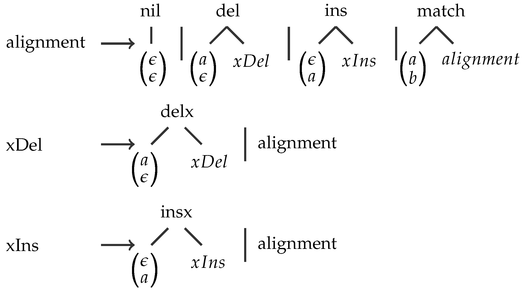
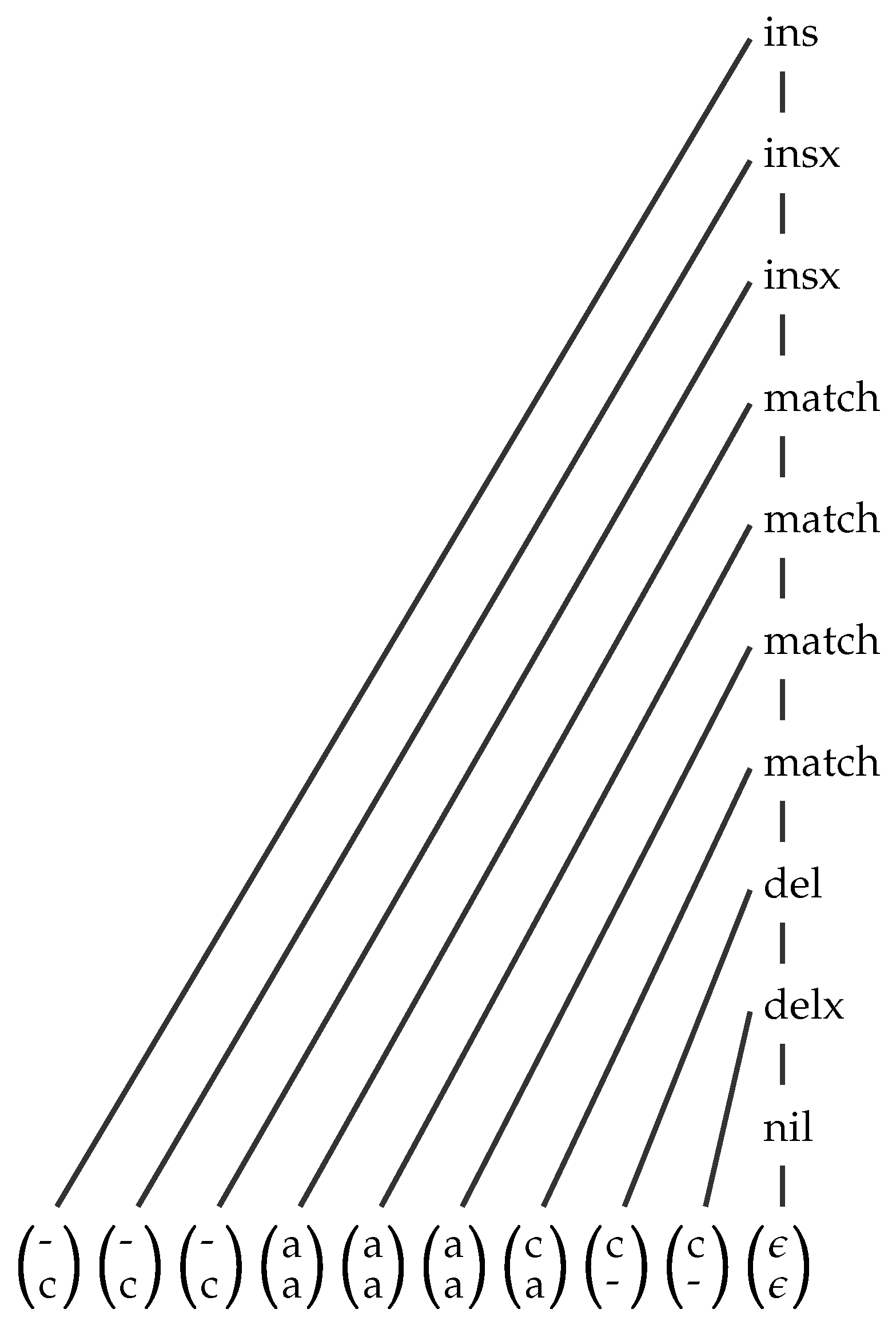
Gotoh’s algorithm: The test case Gotoh2D is an implementation of Gotoh’s algorithm [25] that solves the pairwise sequence alignment problem, also known as string edit distance, for affine gap costs. For Gotoh2D, the gap initiation cost is combined with the gap extension cost in a Pareto product, and the results are printed as an alignment string via a lexicographic product. See our introductory example in Figure 1.

RNA folding: The RNA folding space is defined by the “Overdangle” grammar first described by Janssen et al. [34]. Depending on the application and the number of dimensions in the Pareto product, the folding space is evaluated with different algebras. For Fold2D, we use the minimum free energy (MFE), according to the Turner energy model [35], combined with the maximum expected accuracy (MEA) that consists of the accumulation of base pairs’ probabilities computed with the partition function of the Turner model. For Fold3D, the maximization of the number of predicted base pairs (BP) is added to the Pareto product.

In Prob, we study the integration of reactivity data in RNA secondary prediction with Pareto optimization. The design of algebras is based on distance minimization between probing reactivities (SHAPE [33,36,37], CMCT [38] and DMS [39,40]), using an extended base pair distance following [41]. For Prob2D, the MFE is combined with SHAPE, and for Prob4D, MFE, SHAPE, DMS and CMCT are used. A dot bracket string representation and a RNAshape representation of the candidates of the front are printed via a lexicographic product. A more detailed presentation of probing algebra products will be given in a yet unpublished work [42].

RNA alignment folding: As in test case Ali, we study the behavior of Pareto fronts in an (re-)implementation of RNAalifold [43,44]. We analyze structure prediction with the MFE and MEA algebras and a covariance model algebra COVARfollowing the definitions of [45]. For Ali2D, only MFE is combined with COVAR. For Ali3D, MFE, MEA and COVAR are combined into the Pareto product. Like for the single-sequence RNA folding, a dot bracket string representation and an RNAshape representation of the Pareto front candidates are added via a lexicographic product. It should be mentioned that alignment folding is defined over the same Overdangle grammar as the single sequence case, only now, the input alphabet is columns of aligned characters, including gap symbols. Accordingly, for this case, the Rfam seed alignments are left intact, while for Fold, only the first sequence is used.

4.3. Evaluation of Strategy SORT

Strategy SORT is evaluated in Experiments 1 and 2. Experiment 1 uses two random trials to evaluate the performance of Pareto front computations based on our sorting Algorithm 1–Algorithm 7. For this, we generate lists of sorted sublists of various lengths as inputs and measure their individual runtimes. The outcome is of interest for programmers who consider Pareto optimization, but not necessarily in a dynamic programming context. In an algebraic dynamic programming application, the case of simultaneously merging two or more sorted sublists can occur in Equations (15) and (16). Intermediate results are generated from a search space with particular properties and will be far-from-random datasets. In Experiment 2, we therefore look at our real-world applications, measuring runtimes for each sorting call on intermediate lists of the computations. The outcome is quite different from Experiment 1.

Experiment 1: Two randomized trials were conducted to confirm the viability of all sorted implementations. For this, we uniformly sample data points for $1\le N\le 3000$ (Trial 1) and $1\le N\le$ 20,000 (Trial 2) list elements over $1<M<N$ sorted sublists. M is fixed for each generated input. Trial 1 was ended at 200,990 tests, Trial 2 at 150,505. All list elements have a size of 22 bytes, bigger than most forward computation, but smaller than all backtracing elements in the next experiment set. The times of Algorithms 2–7 were compared against the corresponding times of Algorithm 1, both in total, for all points, as well as utilizing a separator (a separator in algorithmics is a borderline in the data space when one should switch from one algorithm variant to another for best efficiency) on N and M between the sets. All but one algorithm performs either in $O(Nlog(M\left)\right)$ or $O\left(N·M\right)$, compared to $O(Nlog(N\left)\right)$ of Algorithm 1; thus, linear or logarithmic separators should be applied respectively. We tested various parameters of linear and logarithmic functions without the y intercept, as well as constant separators by simple enumeration. In cases where visual inspection showed a possible discordance of this simple model, e.g., in Figure 3a, we manually tested more complex models, however without any improvements. See Table 3.

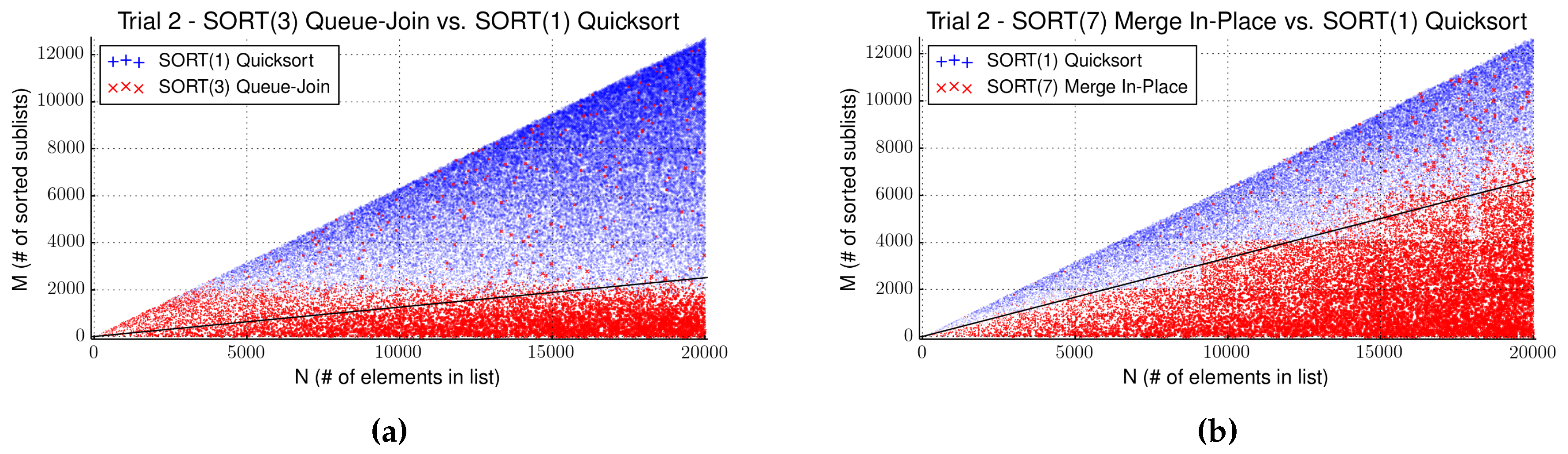
Figure 3. Runtime gain of individual data points of for (a) Algorithm 3 and (b) Algorithm 7 against Algorithm 1 in Trial 2. Points are plotted when one algorithm performed better than the other with point sizes relative to the gained time. Separators are indicated by a black line. In (b), please note that the distribution of red points is less dense above the separator than it is below.

Figure 3. Runtime gain of individual data points of for (a) Algorithm 3 and (b) Algorithm 7 against Algorithm 1 in Trial 2. Points are plotted when one algorithm performed better than the other with point sizes relative to the gained time. Separators are indicated by a black line. In (b), please note that the distribution of red points is less dense above the separator than it is below.

Table 3. Maximal runtime gain of Algorithms 2–7 compared to Algorithm 1 for randomized uniform Trial Sets 1 and 2. The number of comparator calls was averaged over all data points, ignoring separators. Separators indicate where an algorithm becomes superior to Algorithm 1. Separators for runtime gain can operate solely on the total length of the input list N and the number of know nsorted sublists M. They are estimated to the nearest integer for linear separation and to two decimal places for logarithmic separation, in both cases assuming the simplest form without any offset variables.

Algorithm	Avg.Comparator Calls	Max. Saved Time (s)	Separator
Trial 1
Algorithm 1 Quicksort	26,692.7
Algorithm 2 List-Join	1,137,920.0	-	No significant gain
Algorithm 3 Queue-Join	21,780.1	29.0	Always use Algorithm 3
Algorithm 4 In-Join	716,920.0	-	Algorithm 4 never performs consistently better
Algorithm 5 Merge A	18,043.2	11.3	Use Algorithm 5 when $\frac{N}{M}\ge 4$
Algorithm 6 Merge B	18,700.0	7.8	Use Algorithm 6 when $\frac{N}{M}\ge 6$
Algorithm 7 Merge In-Place	18,043.2	13.4	Use Algorithm 7 when $\frac{N}{M}\ge 3$
Trial 2
Algorithm 1 Quicksort	222,480.0
Algorithm 2 List-Join	50,668,600.0	-	No significant gain
Algorithm 3 Queue-Join	181,884.0	33.2	When $\frac{N}{M}\ge 8$
Algorithm 4 In-Join	31,480,100.0	-	Algorithm 4 never performs consistently better
Algorithm 5 Merge A	157,102.0	44.9	Use Algorithm 5 when $\frac{N}{M}\ge 4$
Algorithm 6 Merge B	161,502.0	28.1	Use Algorithm 6 when $\frac{N}{M}\ge 7$
Algorithm 7 Merge In-Place	157,102.0	62.7	Use Algorithm 7 when $\frac{N}{M}\ge 3$

Table 3. Maximal runtime gain of Algorithms 2–7 compared to Algorithm 1 for randomized uniform Trial Sets 1 and 2. The number of comparator calls was averaged over all data points, ignoring separators. Separators indicate where an algorithm becomes superior to Algorithm 1. Separators for runtime gain can operate solely on the total length of the input list N and the number of know nsorted sublists M. They are estimated to the nearest integer for linear separation and to two decimal places for logarithmic separation, in both cases assuming the simplest form without any offset variables.

Algorithm	Avg.Comparator Calls	Max. Saved Time (s)	Separator
Trial 1
Algorithm 1 Quicksort	26,692.7
Algorithm 2 List-Join	1,137,920.0	-	No significant gain
Algorithm 3 Queue-Join	21,780.1	29.0	Always use Algorithm 3
Algorithm 4 In-Join	716,920.0	-	Algorithm 4 never performs consistently better
Algorithm 5 Merge A	18,043.2	11.3	Use Algorithm 5 when $\frac{N}{M}\ge 4$
Algorithm 6 Merge B	18,700.0	7.8	Use Algorithm 6 when $\frac{N}{M}\ge 6$
Algorithm 7 Merge In-Place	18,043.2	13.4	Use Algorithm 7 when $\frac{N}{M}\ge 3$
Trial 2
Algorithm 1 Quicksort	222,480.0
Algorithm 2 List-Join	50,668,600.0	-	No significant gain
Algorithm 3 Queue-Join	181,884.0	33.2	When $\frac{N}{M}\ge 8$
Algorithm 4 In-Join	31,480,100.0	-	Algorithm 4 never performs consistently better
Algorithm 5 Merge A	157,102.0	44.9	Use Algorithm 5 when $\frac{N}{M}\ge 4$
Algorithm 6 Merge B	161,502.0	28.1	Use Algorithm 6 when $\frac{N}{M}\ge 7$
Algorithm 7 Merge In-Place	157,102.0	62.7	Use Algorithm 7 when $\frac{N}{M}\ge 3$

The clear winner in the first trial is Algorithm 3 (Queue-Join), outperforming Quicksort across all tested combinations, followed by Algorithms 5 and 7 with linear separators. In the second trial, Algorithm 3 moves down to third place, overtaken by Algorithms 5 and 7. The reason for this is the bad scaling behavior of Algorithm 3 that becomes apparent when comparing graphs for Algorithms 3 and 7. Both algorithms gain over Quicksort when M is small relative to N and sublists, hence, are long. Figure 3 shows that Algorithm 7 (Merge In-Place) gains more than Algorithm 3 and, hence, performs better on the larger dataset.

For Algorithms 2 and 4, no noticeable gain could be found in any trial, which likely can be attributed to their inferior complexity, showing a drastic increase in comparator calls compared to Algorithm 1. All other algorithms average below Algorithm 1 on comparator calls. Algorithm 6 consistently performs worse than Algorithm 7, the additional tests not yielding any performance boost. In Trial 1, Algorithms 5–7 clearly outperform Algorithm 3 regarding comparator calls while showing longer runtimes. This difference can be explained by the number of memory operations executed by each algorithm. In a randomized setting, only a few elements will be initially placed correctly in the list. Algorithm 3 performs in guaranteed N moves, whereas Algorithms 5–7 take asymptotically $O(Nlog(M\left)\right)$ moves for this case, amortizing the time needed to allocate new memory and destroying the old list on small data.

Experiment 2: Here, we test four dynamic programming applications in biosequence analysis as described earlier in this section. Algorithms 2–4 had exhibited a very bad time behavior in the randomized trials, which is also consistent within all new tested sets, therefore posing a strong limit on testable inputs.

All tests were executed in 2 steps. To achieve an accurate comparison of the sorting algorithms embedded in the application context, first, all implementations of SORT were tested excluding the runtime of the surrounding code, e.g., the iteration through the search space. After identifying the algorithm with the biggest time gain, possibly using a separator, a second test was performed comparing the full running times, including the full GAP-L programs, of all applications. Intermediate N and M or now not uniformly sampled, but arise from the properties of the input and ADP. A summary of the results is presented in Table 4.

Table 4. Summary of computation times and metadata of test cases. Left: Isolated sorting time gains over Algorithm 1. Input length and the final size of the resulting Pareto front are given. Input size denotes the number of characters in the input sequence. Middle: Total runtimes of sorting phase and full Pareto operators, including sorting for the best algorithm. Right: SORT(1) and SORT(7) show the full running times of the basic sorted (Algorithm 1, ${\mathbf{pf}}_{sort}$) and the specialized sorted (Algorithm 7, ${\mathbf{pf}}_{sort}$) implementations.

Name	Input Size	Front Size	Gain (s)	Algorithm	Sort (s)	Pareto (s)	SORT(1) (s)	SORT(7) (s)
Ali2D	509	487	59.1	Algorithm 7	341.9	354.5	579.77	530.0
Gotoh2D	249	209,744	0	Algorithm 7	0.1	0.1	29.42	30.3
Fold2D	509	15	26.8	Algorithm 7	169.9	175.5	334.5	312.3
Fold2D	608	13	304.7	Algorithm 7	1296.1	1305.8	2220.24	1833.3
Prob2D	185	9	0	Algorithm 7	2.1	2.3	3.64	3.6
Ali3D	200	446	0.1	Algorithm 7	0.3	1.2	4.97	4.88
Fold3D	404	165	40.7	Algorithm 7	370.4	727.3	841.64	806.7
Prob4D	185	2327	125.1	Algorithm 7	287.0	1947.9	2556.83	2469.8

Table 4. Summary of computation times and metadata of test cases. Left: Isolated sorting time gains over Algorithm 1. Input length and the final size of the resulting Pareto front are given. Input size denotes the number of characters in the input sequence. Middle: Total runtimes of sorting phase and full Pareto operators, including sorting for the best algorithm. Right: SORT(1) and SORT(7) show the full running times of the basic sorted (Algorithm 1, ${\mathbf{pf}}_{sort}$) and the specialized sorted (Algorithm 7, ${\mathbf{pf}}_{sort}$) implementations.

Name	Input Size	Front Size	Gain (s)	Algorithm	Sort (s)	Pareto (s)	SORT(1) (s)	SORT(7) (s)
Ali2D	509	487	59.1	Algorithm 7	341.9	354.5	579.77	530.0
Gotoh2D	249	209,744	0	Algorithm 7	0.1	0.1	29.42	30.3
Fold2D	509	15	26.8	Algorithm 7	169.9	175.5	334.5	312.3
Fold2D	608	13	304.7	Algorithm 7	1296.1	1305.8	2220.24	1833.3
Prob2D	185	9	0	Algorithm 7	2.1	2.3	3.64	3.6
Ali3D	200	446	0.1	Algorithm 7	0.3	1.2	4.97	4.88
Fold3D	404	165	40.7	Algorithm 7	370.4	727.3	841.64	806.7
Prob4D	185	2327	125.1	Algorithm 7	287.0	1947.9	2556.83	2469.8

Looking at the sorting performance alone, a clear speed up over Algorithm 1 could be achieved for most test cases. Exceptions are Ali3D and Prob2D, both of which have a very low overall computation time, and Gotoh2D. In all cases, Algorithm 7 (Merge In-Place) was the best performing algorithm. Furthermore, in contrast to the randomized trials, no separator was needed to optimize runtimes. Algorithm 5 performed second without any exceptions in the tested sets. While Algorithm 3 had appeared promising in the randomized trials, only for Prob4D could a separator be found, such that Algorithm 3 could achieve a runtime gain, even though it was significantly lower than that of Algorithm 7. Like in the randomized trials, Algorithm 6 performed consistently worse than Algorithms 2, 4, and 5, never achieving any gain.

Neither input size nor front size seem to be a good indicator on which algorithm works best. Most noticeably, the largest gain over Algorithm 1 was achieved with a final front size of 13 for Fold2D. For Ali3D, there was nearly no gain, despite a much larger final front size of 446. Prob4D and Ali3D were executed on similarly-sized inputs, but only one could achieve a significant gain. The reason for these observations is that no direct statements can be made about intermediate lists and front sizes from input size or final front size alone. Pareto fronts may grow and shrink in the course of the computation.

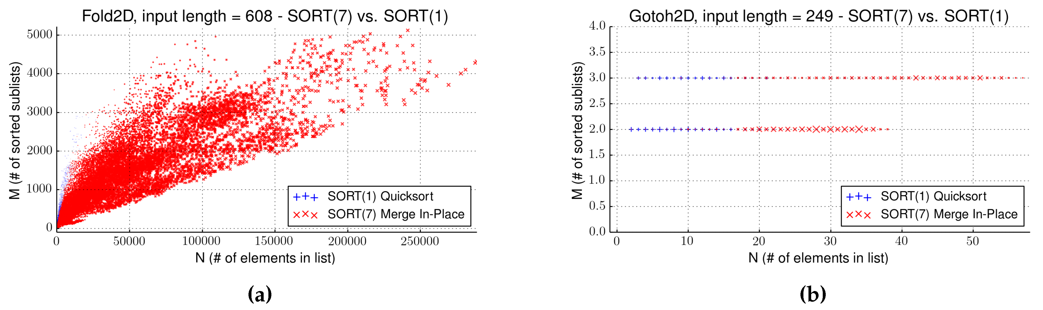
Most informative is the layout of the search space. In Figure 4, the scatter plots for Fold2D, showing the best improvement, and Gotoh2D, with no improvement, are presented. In its moderate computation time and large final front size, Gotoh2D shows only very limited variance for intermediate results. The final Pareto front consists mostly of co-optimumsthat are only added in the last step of the computation and are not present for the sorting phases. Comparing the full computation times of Gotoh2D, the overall time variance is minimal. The reason for this is the problem decomposition of Gotoh2D. At most 3 sorted sublists are combined by the tree grammars, while the evaluation algebra also does not allow for much variation. In contrast, the grammars for the other applications have at least one rule that generates sublists of a length proportional to the input length. We will later revisit this analysis when comparing the runtime of all algorithms.

Comparing the total running time of the isolated sorting phases and full Pareto computations shows that for almost all cases, more than half of the total computation time is spent in the Pareto operators. Gotoh2D is again the only exception, following the same rationale as above. While the sorting phases seem to take up the most time of the computations for 2-dimensional cases, the gap grows larger for higher dimensions.

Figure 4. Runtime gain of individual data points of Algorithm 7 against Algorithm 1 for the test cases (a) Fold2D and (b) Gotoh2D. Points are plotted when one algorithm performed better than the other with point sizes relative to the gained time. Gotoh2D shows only very little variance in list sizes contrary to Fold2D, explaining the performance differences.

Figure 4. Runtime gain of individual data points of Algorithm 7 against Algorithm 1 for the test cases (a) Fold2D and (b) Gotoh2D. Points are plotted when one algorithm performed better than the other with point sizes relative to the gained time. Gotoh2D shows only very little variance in list sizes contrary to Fold2D, explaining the performance differences.

4.4. Strategy EAGER

In Experiment 3, we evaluate the strategy EAGER with respect to its two variants: EAGER (sorted) uses Merge 1 and Merge 2, while EAGER (unsorted) uses Merge 3. We compare the overall runtimes, and here, we obtain a clear picture: with 2 dimensions, EAGER (sorted) is superior to EAGER (unsorted), from almost equal up to a factor of 2. With higher dimension, EAGER (unsorted) becomes increasingly faster. This is consistent with the statement in Section 3 that lexicographic sorting no longer implies an order in the second to highest dimensions. Therefore, this cannot be exploited, and the whole sorting does not pay off. The concrete measurements are included below in Table 6.

4.5. Comparing Two Sorting Strategies

In Experiment 4, we test the sorted variant of strategy EAGER on the same four ADP applications as before and compare it to the simplest version of SORT, i.e., SORT(1), which uses the off-the-shelf Quicksort algorithm. Our goal is to find possible separators, where one method becomes better than the other, suggesting a data-dependent switch between methods (as we did in Experiment 1). Again, the tests were executed in 2 steps, first comparing the runtimes at the level of intermediate subproblems, excluding the runtime of the surrounding code, and afterwards comparing the full running times of the best implementations. As separators, linear and exponential separations based on values of N and M are considered, motivated by the asymptotic complexity of the compared implementations that differ in the factors of these two variables. A summary of the results is shown in Table 5.

Table 5. Summary of computation times and metadata of test cases. Left: Isolated sorting time gains over Algorithm 1 with the total sum of running times for Merge 1 or Merge 2, respectively (Sort). Input length and the final size of the resulting Pareto front are given. Input size denotes the number of characters in the input sequence. Right: SORT(1) and EAGER(sort) show the full running times of the basic sorted (Algorithm 1, ${\mathbf{pf}}_{sort}$) and the Pareto-eager implementations (Merge 1 or Merge 2 respectively).

Name	Input Size	Front Size	Gain (s)	Separator	Sort (s)	SORT(1) (s)	EAGER(sort) (s)
Ali2D	509	487	220.46	-	220.1	579.77	356.11
Gotoh2D	249	209,744	-	-	0.1	29.42	29.83
Fold2D	608	13	762.16	-	542.3	2220.24	1054.39
Prob2D	185	9	0	-	1.7	3.64	2.76
Ali3D	200	446	-	-	4.3	4.97	8.04
Fold3D	404	165	-	-	5757.9	841.64	5810.36
Prob4D	185	2327	-	-	14,442.3	2556.83	14,552.12

Table 5. Summary of computation times and metadata of test cases. Left: Isolated sorting time gains over Algorithm 1 with the total sum of running times for Merge 1 or Merge 2, respectively (Sort). Input length and the final size of the resulting Pareto front are given. Input size denotes the number of characters in the input sequence. Right: SORT(1) and EAGER(sort) show the full running times of the basic sorted (Algorithm 1, ${\mathbf{pf}}_{sort}$) and the Pareto-eager implementations (Merge 1 or Merge 2 respectively).

Name	Input Size	Front Size	Gain (s)	Separator	Sort (s)	SORT(1) (s)	EAGER(sort) (s)
Ali2D	509	487	220.46	-	220.1	579.77	356.11
Gotoh2D	249	209,744	-	-	0.1	29.42	29.83
Fold2D	608	13	762.16	-	542.3	2220.24	1054.39
Prob2D	185	9	0	-	1.7	3.64	2.76
Ali3D	200	446	-	-	4.3	4.97	8.04
Fold3D	404	165	-	-	5757.9	841.64	5810.36
Prob4D	185	2327	-	-	14,442.3	2556.83	14,552.12

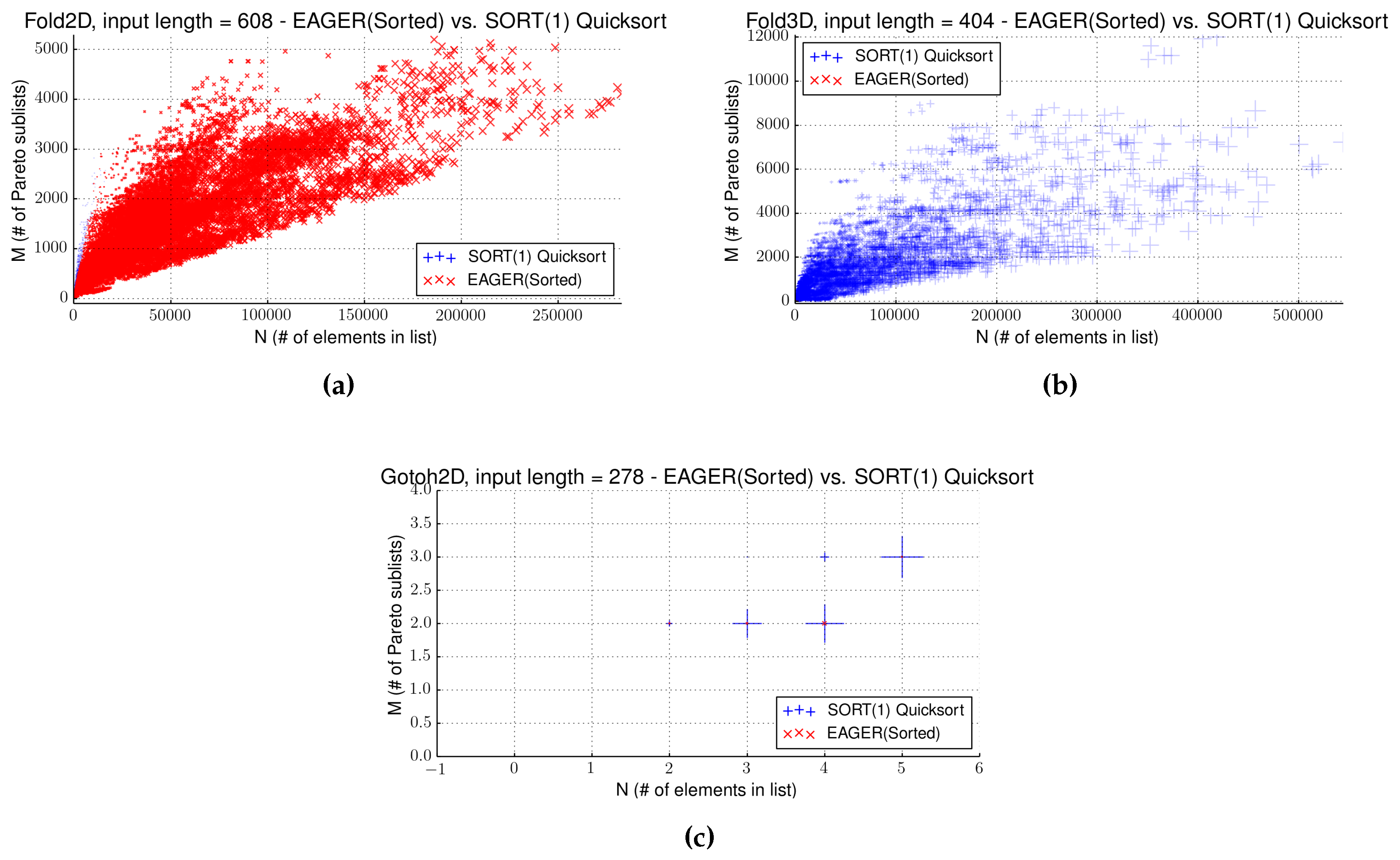
There are two main observations. First of all, no separators are given for any case. The reason for this is that in no case could any improving separators be found. In all cases, one algorithm performs best for all data points. Secondly, with the exception of Gotoh2D, for two-dimensional definitions, EAGER(sorted) always performed best, whereas for higher dimensions, SORT(1) is superior without failure. The explanations for both facts are not entirely unrelated. The difference between dimensions is of course a result of the different underlying implementations of Merge 1 and Merge 2.

As before, we see that more than half of the full running times are spent in Pareto operators.

The two-dimensional case is very similar to the sorted case, only that we apply Pareto operators, as well as sorting the elements. In a way, Merge 1 works similar to a normal two-way merge sort with a merge step definition that is not in place, reflected by the complexity of $O(Nlog(M\left)\right)$. By the same arguments as before, Merge 1 is likely to perform better than executing a sorting in $O(Nlog(N\left)\right)$ when $M<<N$. Conversely, if the number of sublists M is near the number of elements N and sublists are very short, the sorted case with Algorithm 1 will perform better. As intermediate lists are created by combining sub-results, the lengths of individual sub-results are likely to stay over a certain threshold that seems to be high enough in order for Merge 1 to perform well.

For higher dimensions, the situation changes, as now both algorithms perform in $O\left(N^2\right)$, the complexity of the Pareto operations now dominating the sorting aspects of both implementations. However, the additional factors brought in by the different scenarios strongly favor the use of Algorithm 1 and a single operator step, compared to multiple smaller operator steps, each in $O\left(N^2\right)$. This seems to be true already for small N and, accordingly, only grows worse for longer candidate lists. The scatter plots in Figure 5a,b confirm this theory for both cases.

Figure 5. Runtime gain of individual data points of SORT(1) against EAGER(sorted) for the test cases (a) Fold2D and (c) Gotoh2D and for (b) Fold3D. Points are plotted when one algorithm performed better than the other with point sizes relative to the gained time. For the two-dimensional Fold2D, EAGER(sorted) performs best. For the three-dimensional Fold3D, SORT(1) always performed better. For Gotoh, the plot shows only limited variation and no winning algorithm.

Figure 5. Runtime gain of individual data points of SORT(1) against EAGER(sorted) for the test cases (a) Fold2D and (c) Gotoh2D and for (b) Fold3D. Points are plotted when one algorithm performed better than the other with point sizes relative to the gained time. For the two-dimensional Fold2D, EAGER(sorted) performs best. For the three-dimensional Fold3D, SORT(1) always performed better. For Gotoh, the plot shows only limited variation and no winning algorithm.

Like in the sorted scenario, Gotoh2D shows hardly any variation in the computation times. Of course, the same rationale as before applies to explain this behavior. As we can see in Figure 5c, due to the Pareto condition, intermediate lists are even shorter and allow even fewer variations and with even less potential for better performing algorithms.

4.6. Putting It All Together

Now that all individual components have been established in the previous sections, it is time to combine the results of the previous experiments and relate them to strategy NOSORT. We write simply NOSORT for the variant using ${\mathbf{pf}}_{nosort}$ and NOSORT(B) using ${\mathbf{pf}}_{bentley}$.

In Experiment 5, only full runtimes are considered, including all recursions of the ADP programs, production of output, etc. A summary of all runtimes over all applications is presented in Table 6. We will analyze the data in multiple steps, referencing results from previous subsections as needed.

Table 6. Summary of benchmarks of all applications. Input and front sizes are given. We compare the full runtimes in seconds (s) for three strategies in overall six variants: the strategy (NOSORT) using ${\mathbf{pf}}_{nosort}$, its multidimensional variant NOSORT(B) using ${\mathbf{pf}}_{bentley}$, SORT(1) using Quicksort and ${\mathbf{pf}}_{sort}$, the specialized sorted case SORT(7), using Merge-in-place with ${\mathbf{pf}}_{sort}$, as well as EAGER (Sorted), using Merge 1 and Merge 2, and, finally, EAGER(Unsorted), using Merge 3. No algorithm can win in all cases.

Name	Input	Front	NOSORT	NOSORT(B)	SORT(1)	SORT(7)	EAGER(Sort.)	EAGER(Uns.)
Ali2D	509	487	667.84	-	579.77	529.98	356.11	775.77
Gotoh2D	249	209,744	29.19	-	29.42	30.32	29.83	29.75
Fold2D	509	15	154.12	-	334.53	312.28	216.54	228.29
Fold2D	608	13	631.43	-	2220.24	1833.31	1054.39	1279.03
Prob2D	185	9	2.05	-	3.64	3.6	2.76	2.36
Ali3D	200	446	5.43	4.93	4.97	4.88	8.04	4.85
Fold3D	404	165	314.52	704.03	841.64	806.67	5810.36	813.2
Prob4D	185	2327	1774.88	1227.13	2556.83	2449.83	14,552.12	2535.11

Table 6. Summary of benchmarks of all applications. Input and front sizes are given. We compare the full runtimes in seconds (s) for three strategies in overall six variants: the strategy (NOSORT) using ${\mathbf{pf}}_{nosort}$, its multidimensional variant NOSORT(B) using ${\mathbf{pf}}_{bentley}$, SORT(1) using Quicksort and ${\mathbf{pf}}_{sort}$, the specialized sorted case SORT(7), using Merge-in-place with ${\mathbf{pf}}_{sort}$, as well as EAGER (Sorted), using Merge 1 and Merge 2, and, finally, EAGER(Unsorted), using Merge 3. No algorithm can win in all cases.

Name	Input	Front	NOSORT	NOSORT(B)	SORT(1)	SORT(7)	EAGER(Sort.)	EAGER(Uns.)
Ali2D	509	487	667.84	-	579.77	529.98	356.11	775.77
Gotoh2D	249	209,744	29.19	-	29.42	30.32	29.83	29.75
Fold2D	509	15	154.12	-	334.53	312.28	216.54	228.29
Fold2D	608	13	631.43	-	2220.24	1833.31	1054.39	1279.03
Prob2D	185	9	2.05	-	3.64	3.6	2.76	2.36
Ali3D	200	446	5.43	4.93	4.97	4.88	8.04	4.85
Fold3D	404	165	314.52	704.03	841.64	806.67	5810.36	813.2
Prob4D	185	2327	1774.88	1227.13	2556.83	2449.83	14,552.12	2535.11

The most noticeable observation that can be made from the data is that with two exceptions, NOSORT performs best, both for two-dimensional and higher-dimensional cases. This replicates the results of the preliminary implementations done in [21]. There, the authors suggest that this good behavior can be attributed to a positive randomization effect. When operating on sorted lists, extremal points of the Pareto fronts that are maximal in one dimension, but minimal in others, will be tested first. Such a point is unlikely to create domination over a new element, as it dominates only a rather small volume in the space of possible values. On unsorted lists, non-extremal points are on average encountered earlier, and thus, domination can be established earlier in the computations. Further tests seem to hint at this theory, but a proof appears hard to construct. In particular, we see two points in our measurements that challenge this hypothesis: (1) one would expect EAGER (unsorted) to beat EAGER (sorted) for the same reason, but this is not the case; and (2) EAGER (sorted) clearly beats NOSORT on problem Ali2D, which would then have to be attributed to a special property of its search space.

Although EAGER (unsorted) improves over EAGER (sorted) on multi-dimensional problems, it shows no significant advantage when compared to all other methods. It only wins by a small margin on problem Ali3D. In contrast, except for two cases with very small overall computation times like Ali3D and Gotoh2D, all other uses show a significant increase in running times. This behavior can likely be explained by differences in the implementation that were needed for the Pareto-eager strategies compared to the standard implementation of ADP, introducing new factors to the runtime that could not be amortized by removing candidates earlier on.

Let us now consider the problems Ali2D and Ali3D, where NOSORT could not perform best. For Ali2D, instead, EAGER (sorted) was consistently better. At the same time, both SORT strategies performed better than NOSORT, as well. This is a unique case within all other test cases. The two facts are not without a deeper connection, however. We already saw that for all cases, SORT(7) (using Merge-in-place) can improve the runtime compared to SORT(1) (using Quicksort). Only for the Ali problems, where SORT(1) already performs better than NOSORT, SORT(7) can increase the overall implementation time even more. Here, however, the two-dimensional sorted case EAGER (sorted) becomes the best. A likely reason for these particular measurement, with the only winning point of EAGER (sorted), is that sorting implementations all profit from the same properties of the search space that allow an effective merge of presorted lists. At least in this case, the Pareto eager implementation seems to benefit the strongest. The early reduction of candidate lists is the most likely reason for this good performance.

Altogether, our findings do not imply that the SORT strategies are without merit. Although EAGER (unsorted) beats it for Ali3D as an outlier, the good effect of the sorted implementation compared to the standard NOSORT can be seen here, as well. Due to its increased implementation complexity, EAGER (sorted) cannot really be preferred over SORT(7). EAGER (unsorted) is unlikely to scale well. For Ali3D and similar cases, and still for larger inputs, sorted SORT(7) can be expected to be the best option.

4.7. Influence of Search Space Properties and Dimensionality

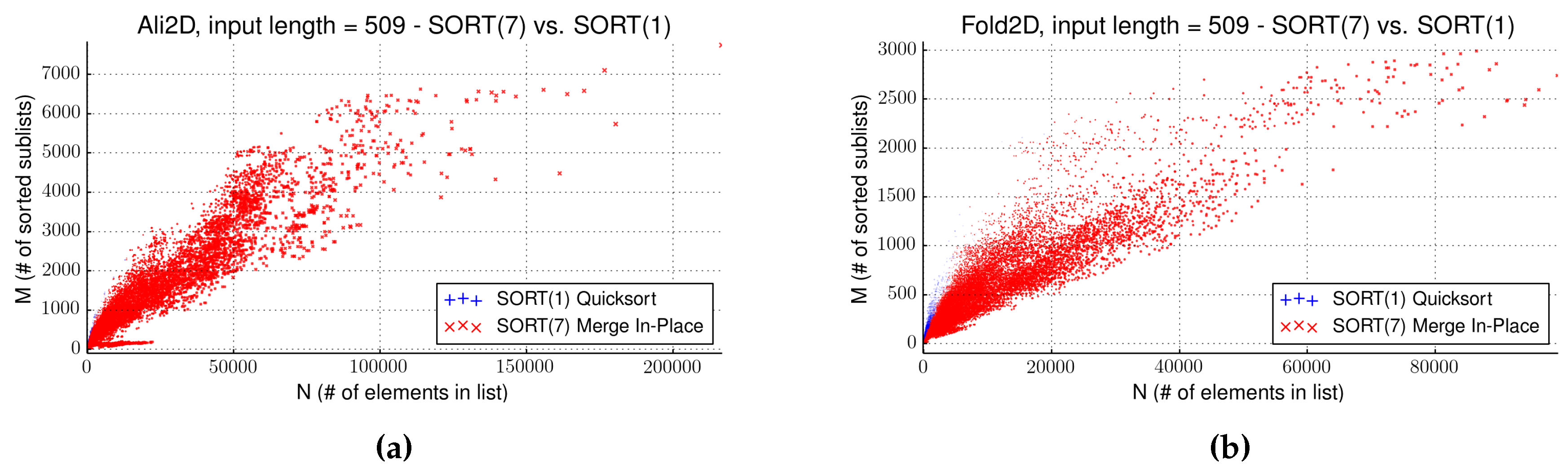
Finally, we look at the effect of the search space decomposition and the performed evaluation. So far, our discussion lacks an explanation of why problems Ali2D and Ali3D behave differently from all other applications. For this, it is time to return to the layout of the search space. Figure 6 shows the plots of intermediate lists for the sorted cases of Ali2D and Fold2D. Ali2D and Fold2D were computed out of the same data and use the same tree grammar (i.e., they perform the same search space decomposition), employing the same number of evaluation algebras. The difference in the distribution of data points is therefore caused by the qualitative influence of the evaluation algebras. They solve a different problem: Ali2D reads aligned sequences and folds them, Pareto-optimizing sequence similarity and free energy. Fold2D looks only at a single sequence (Yes, this is described by the same tree grammar in both problems. Only the terminal alphabet has been exchanged. Re-use of algorithm components is a big issue in ADP.) and folds it, Pareto-optimizing over free energy and chemical probing evidence.

Figure 6. Runtime gain of individual data points of SORT(7) against SORT(1) for (a) Ali2D and (b) Fold2D. Points are plotted when one algorithm performed better than the other with point sizes relative to the gained time. The point of interest here is not performance, but the observation that both problems produce intermediate results of significantly different sizes.

Figure 6. Runtime gain of individual data points of SORT(7) against SORT(1) for (a) Ali2D and (b) Fold2D. Points are plotted when one algorithm performed better than the other with point sizes relative to the gained time. The point of interest here is not performance, but the observation that both problems produce intermediate results of significantly different sizes.

Empirically, we find (Figure 6) that Fold2D generates smaller lists, with (in relation to) fewer sublists compared to Ali2D. This alone, however, cannot explain why for Ali2D, consistently, EAGER (sorted) performs best, while for Fold2D, the strategy NOSORT is considerably faster. This discrepancy must be related to the order and sortedness in which candidates are created, sortedness addressing how many elements are inverted in the lists upon creation.

Using different search space decompositions has an even more dramatic effect. This becomes apparent when taking another look at application Gotoh2D. We already saw in the previous section that Gotoh2D deviates strongly from all other cases, limiting the variation within intermediate candidate lists (see Figure 4b and Figure 5c). With all folding problems, the size of the search space depends on the input, and variance is high. The number of sublists also depends on input length. With sequence alignment, in contrast, the number of candidates in the search space only depends on the length of the sequences, not on their content, and the number of sublists is always ≤3. This reflects on the very limited time difference for not just the sorted and Pareto-eager implementation, but all tested algorithms.

The curse of dimensionality calls for its tribute. Of all applications, Prob4D was the only case to define a Pareto product over four dimensions, and because of this, it is also exhibiting very long intermediate lists. As such, Prob4D was the only case where the superior asymptotic complexity of the NOSORT(B) using ${\mathbf{pf}}_{bentley}$ resulted in an actual performance increase. It is interesting to note that Fold3D also exhibited similarly-sized intermediate lists for the largest input, but instead of improving runtimes, ${\mathbf{pf}}_{bentley}$ doubled the effort. In its complicated definition, ${\mathbf{pf}}_{bentley}$ employs high internal factors for runtime that can only be overcome for large inputs. Higher dimensional products are more likely to fulfil this property.

5. Conclusions

The most important finding of our study is that the best strategy for integrating Pareto optimization depends greatly on the dynamic programming problem to be solved. Not only the dimensionality of the Pareto optimization, but also the nature of the search space decomposition and properties of the evaluation objectives can drastically influence efficiency. Dynamic programming is a wide field, and while we can give some guidance for problems similar to the ones studied here, in general, a good implementation will require some engineering and experimentation. The most surprising observation, although already hinted at in [21], is that the “naive” strategy NOSORT performs well in so many cases. This calls for a deeper expected case analysis, which we pose as an open problem here.

We will structure our advice in two sections, one for users of a dynamic programming framework, such as Bellman’s GAP (or of other frameworks, once they support Pareto optimization), and one for the hard-working, hand coding dynamic programmer.

5.1. Using Pareto Products in Bellman’s GAP

Our experience has led to the extension of Bellman’s GAP in the following way:

• Bellman’s GAP provides a single operator in GAP-L to express Pareto products of evaluation algebras in the form $(\mathcal{A}^\mathcal{B})$ and for higher dimensions as $(\mathcal{A}^\mathcal{B}^\mathcal{C}^\mathcal{D})$. The compiler can switch between code generation for the two- and the multi-dimensional case.
• Different strategies, NOSORT, NOSORT(B), SORT(1), SORT(7), EAGER (sorted) and EAGER (unsorted), are available via compilation switches. Thus, GAP-L source code does not need to be changed when exploring different strategies.
• If nothing is known about the peculiarities of the application, we recommend to start out with strategy NOSORT. If this does not solve the problem to satisfaction, other strategies should be tried.

5.2. Hand Coding Pareto Optimization into a Dynamic Programming Algorithm

Hand coding Pareto optimization in a dynamic programming context is a major challenge. Dynamic programming algorithms are intrinsically difficult to debug, since a subscript error in the recurrences may merely lead to overlooking the optimal solution, once in a while. On top of that, one now has to deal with multiple solutions, with sorting or merge-in-placeoperations. How can one tell that some solutions should be in the Pareto front, but have been lost along the way? Here is our first advice:

• First of all, consider the possibility of abandoning hand coding and evaluate the suitability of Bellman’s GAP for the purpose. Even when you have already coded the equivalent of $\mathcal{G}(A,x)$ and $\mathcal{G}(B,x)$, reformulating your program in ADP will be faster and less error-prone than modifying your source code towards the equivalent of $\mathcal{G}(\mathcal{A}^\mathcal{B})$. Doing so, you get a correct Pareto implementation for free. Keep in mind that with hand coding, you also have to implement the backtracing of Pareto-optimal solutions (i.e., the solution candidates behind the Pareto-optimal scores), while Bellman’s GAP also generates the backtracing phase for you.

The reminder of our advice addresses the situation where hand coding appears unavoidable.

• Aim first for an implementation of the NOSORT strategy. It is the simplest to implement and was a good choice in most of our test cases.
• Use an abstract data type to interface recurrences and scoring functions.
• Provide separate implementations for evaluating under scoring systems A and B first, and test them thoroughly.
• Then, implement the equivalent of $(\mathcal{A}^\mathcal{B})$. For debugging, make use of the mathematical fact that the optima under A and B must show up as the extreme points in the Pareto front under $(\mathcal{A}^\mathcal{B})$.
• If efficiency is problematic and you are going to implement another strategy X, make use of the property that NOSORT and strategy X must produce the identical Pareto fronts on the same input.
• If you choose to implement a sorting strategy, keep in mind our observation that sorting algorithm performance on random data is not meaningful for deciding on its use in the dynamic programming context. Use off-the-shelf Quicksort, or Merge-in-place if memory is critical.

Finally, users of Bellman’s GAP, as well a hand coding dynamic programmer should be aware of the following caveat when implementing and comparing several strategies.

• All dynamic programming with multiple solutions is based on the law of (strict) monotonicity, which all scoring functions must obey. Floating point errors can obstruct this prerequisite with functions that mathematically obey it.

To illustrate the above: consider computing with two decimal positions. When scores 1.00 and 1.01 are both multiplied by 0.4, they both come out as 0.40. Now, let there be sub-solutions with scores (11, 1.00) and (10, 1.01). Neither dominates the other. After extending the sub-solutions, we obtain scores (4.4, 0.40) and (4.0, 0.40). Now, the first dominates the second, and a solution is lost that should mathematically be in the Pareto front. We found that this effect does rarely show up in practice. However, it does occur occasionally, and this matters to the program developer. When you write a large test suite that tests different strategies for identical Pareto fronts, which mathematically they must deliver, be aware that occasional discrepancies may indicate rounding effects and not a flaw in your implementation.

5.3. Outlook

While algebraic dynamic programming in general and Bellman’s GAP more recently have proven suitable for numerous bioinformatics applications, there is the more powerful (but yet un-implemented) framework of inverse coupled rewrite systems (ICOREs) [11]. This defines algebraic dynamic programming also on tree-structured data. While we conjecture that a Pareto product preserves Bellman’s principle also in this framework, it is not clear if any of our empirical observations on implementation strategies carry over. Recurrences for dynamic programming over trees tend to be more sophisticated compared to those in sequence analysis, and we have learned here that the shape of the recurrences can have a drastic effect on the relative performance of strategies.

Another problem open so far is the influence of parallelization on Pareto operators. Within Bellman’s GAP, OpenMP can be used to parallelize the dynamic programming recursions [46]. This, however, will have no influence on the relative speed of the Pareto operators, but still can improve the overall runtime. Additionally, for the NOSORT(B), SORT and EAGER strategies, easy parallelizations could be constructed that remain yet to be explored.