Offset-Assisted Factored Solution of Nonlinear Systems

Abstract

This paper presents an improvement to the recently-introduced factored method for the solution of nonlinear equations. The basic idea consists of transforming the original system by adding an offset to all unknowns. When searching for real solutions, a real offset prevents the intermediate values of unknowns from becoming complex. Reciprocally, when searching for complex solutions, a complex offset is advisable to allow the iterative process to quickly abandon the real domain. Several examples are used to illustrate the performance of the proposed algorithm, when compared to Newton’s method.

1. Introduction

Numerically finding the solutions of nonlinear equation systems constitutes both a critical and challenging task in many engineering and scientific disciplines [1]. According to John Rice, who coined the term mathematical software in 1969, “solving systems of nonlinear equations is perhaps the most difficult problem in all of numerical computations” [2].

Among the plethora of procedures developed over the last three centuries for the solution of nonlinear systems [3,4], Newton’s method stands out as the best general-purpose iterative algorithm, trading off simplicity and reliability, particularly when reasonable initial guesses can be made [5,6].

Even though most existing methods for solving nonlinear equations preserve the structure of the original system throughout the solution process, it has long been known that better convergence rates or wider basins of attractions can be achieved by previously rearranging nonlinear systems. According to [7] (pp. 174–176), “the general idea is that a global nonlinear transformation may create an algebraically equivalent system on which Newton’s method does better because the new system is more linear. Unfortunately, there is no general way to apply this idea; its application will be problem-specific”.

Recently, the idea of transforming nonlinear systems to enhance the solution process has been systematically exploited by the so-called factored solution approach [8]. It consists of unfolding the nonlinear system by preliminarily identifying all distinct nonlinear terms, each deemed a new variable. This leads to an augmented system, composed of two sets of linear equations along with a one-to-one nonlinear mapping with the explicit inverse. The resulting procedure involves three steps at each iteration: (1) solution of the least-distance linear problem; (2) nonlinear trivial transformation; (3) computation of a Newton-like step.

The factored procedure has been successfully applied to large-scale power systems problems [9], generally showing wider basins of attractions than Newton’s method while preserving its quadratic convergence rates near the solution. Moreover, in large-scale engineering applications, the factored method has proven to be capable of reliably converging to complex solutions when real solutions do not exist [10].

In the presence of nonlinear terms comprising products of variables, very commonly found in practice, the factored approach has to resort to the log please check the use of italics for the term throughout version of the involved variables, so as to transform the original system into a suitable canonical form [8]. For systems of equations with positive real solutions, this procedure performs satisfactorily. However, when searching for negative or complex solutions, the use of log functions sometimes lead to oscillatory or unexpected behavior.

This article proposes a straightforward modification to the factored solution procedure allowing negative real or complex solutions to be safely handled. The idea is to transform the original system by simply adding an offset to those variables involved in log expressions. A large enough positive real offset prevents intermediate values from becoming negative throughout the solution process, significantly enhancing the capability of the factored approach to reach negative real solutions. When needed, convergence to complex solutions can be also assured, or at least enhanced, by adding an imaginary component to the offset. Several benchmark examples are used to illustrate the proposed methodology and compare its performance to that of Newton’s method.

2. Review of the Factored Solution Method

The aim of this section is to briefly review the factored solution approach recently introduced in [8]. Consider a general nonlinear system, compactly written as follows:

$$h\left(x\right)=p$$

(1)

where $p\in {\mathbb{R}}^n$ is a given parameter vector and $x\in {\mathbb{R}}^n$ is the unknown vector.

Newton’s method approaches a solution from an initial guess, $x_0$, by successively solving:

$$H_k\Delta x_k=\Delta p_k$$

(2)

where subindex k denotes the iteration counter, $\Delta x_k=x_{k+1}-x_k$, $H_k$ is the Jacobian of $h(·)$, computed at the current point $x_k$, and $\Delta p_k=p-h\left(x_k\right)$ is the mismatch vector.

The factored solution method assumes that suitable auxiliary vectors, y and $u\in {\mathbb{R}}^m$, with $m>n$, can be introduced so that the original Equation system(1) can be unfolded into three simpler problems:

$$\begin{array}{ccc}\hfill Ey& =& p\hfill \end{array}$$

(3)

$$\begin{array}{ccc}\hfill u& =& f\left(y\right)\hfill \end{array}$$

(4)

$$\begin{array}{ccc}\hfill Cx& =& u\hfill \end{array}$$

(5)

where E and C are rectangular matrices of sizes $n\times m$ and $m\times n$, respectively, and vector $f(·)$ comprises a set of one-to-one nonlinear functions, also known as a diagonal nonlinear mapping [11],

$$u_i=f_i\left(y_i\right);i=1,\cdots m$$

(6)

each with the closed-form inverse,

$$y_i=f_i^{-1}\left(u_i\right)\Rightarrow y=f^{-1}\left(u\right)$$

(7)

By eliminating vector u the above system can also be written in more compact form:

$$\begin{array}{ccc}\hfill Ey& =& p\hfill \end{array}$$

(8)

$$\begin{array}{ccc}\hfill Cx& =& f\left(y\right)\hfill \end{array}$$

(9)

It is worth noting that Equation (8) is a linear underdetermined system, while Equation (9) is an overdetermined one. Among the infinite solutions to Equation (8), only those exactly satisfying Equation (9) constitute solutions to the original nonlinear Equation system (1). As explained in [8], many systems can be found in practice to which such a factorization can be applied, either directly or after trivial algebraic manipulations transforming the original system into suitable canonical forms.

The augmented Equation systems (3)–(5) can be efficiently solved as follows (the reader is referred to [8], where the solution procedure below is developed from scratch as an optimization problem):

• Step 0: Given an initial guess, $x_0$, set $y_k=f^{-1}\left(C{x}_0\right)$.
• Step 1:

  • 1.1. Compute λ by solving the linear system,

    $$\left(E{E}^T\right)\lambda =p-E{y}_k$$

    (10)
  • 1.2. Obtain $\tilde{y}$ from,

    $$\tilde{y}=y_k+E^T\lambda$$

    (11)
• Step 2: Perform the one-to-one nonlinear transformation, $\tilde{u}=f\left(\tilde{y}\right)$, and obtain the (trivial) inverse of the diagonal Jacobian matrix, ${\tilde{F}}^{-1}$.
• Step 3:

  • 3.1. Obtain $x_{k+1}$ by solving,

    $$\underset{\tilde{H}}{\underbrace{E{\tilde{F}}^{-1}C}}{x}_{k+1}=E{\tilde{F}}^{-1}\tilde{u}$$

    (12)
  • 3.2. Update $y_{k+1}=f^{-1}\left(C{x}_{k+1}\right)$.
  • 3.3. Convergence check: if $\left|\right|p-E{y}_{k+1}{\left|\right|}_{\infty }<\epsilon$, then stop; else, return to Step 1.

Step 1 provides a new vector $\tilde{y}$ that, satisfying Equation (8), minimizes the distance to the previous value $y_k$. The computational cost of this step is very small provided the Cholesky factors of $E{E}^T$ were saved during the first iteration, and the mismatch vector, $p-E{y}_k$, is taken from the previous execution of Step 3.3. It is worth noting that the Jacobian matrix $\tilde{H}$ in Step 3.1 has the same structure as the one involved in Newton’s method, Equation (2), but it is computed at a different point.

Tests performed so far with the factored method on large realistic problems [9] have shown that each iteration of the above factored procedure is generally faster than that of Newton’s method. Moreover, as shown in [8], the factored method exhibits a quadratic convergence rate in the neighborhood of a solution and wider basins of attractions. An outstanding additional feature of the factored method is that, unlike Newton’s method, it can converge to complex solutions when the initial point is not in the basin of attraction of a real solution or simply when real solutions do not exist at all [10].

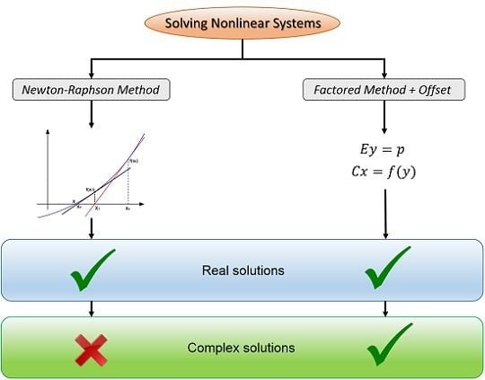
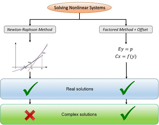
3. Limitations of the Factored Method When Real Negative or Complex Solutions Are Involved

When the nonlinear system to be solved contains terms of the form $x_i^a{x}_j^b$, the application of the factored method requires that the original set of variables be replaced by its log counterpart [8],

$${\alpha }_i=ln{x}_{i}i=1,\cdots ,n$$

Then, each distinct term $x_i^a{x}_j^b$ gives rise to a new auxiliary variable $y_{ij}$,

$$y_{ij}=x_i^a{x}_j^b=exp(a{\alpha }_i+b{\alpha }_j)$$

In this particular case, the corresponding component of the nonlinear relationship $u=f\left(y\right)$ reduces to,

$$u_{ij}=ln{y}_{ij}\Rightarrow y_{ij}=exp{u}_{ij}$$

which leads to a linear relationship, $u=C\alpha$, as required by the last step,

$$u_{ij}=a{\alpha }_i+b{\alpha }_j$$

In those cases in which all solutions of the nonlinear system in hand are real and positive, the use of the log function does not usually pose any problem. However, in the presence of negative or complex solutions, it has been found experimentally that the performance of the factored method is not always as good, leading in many cases to oscillatory or erratic behavior. In what follows, the nature of this drawback is analyzed, and ways of circumventing it when searching for negative and complex solutions are separately discussed.

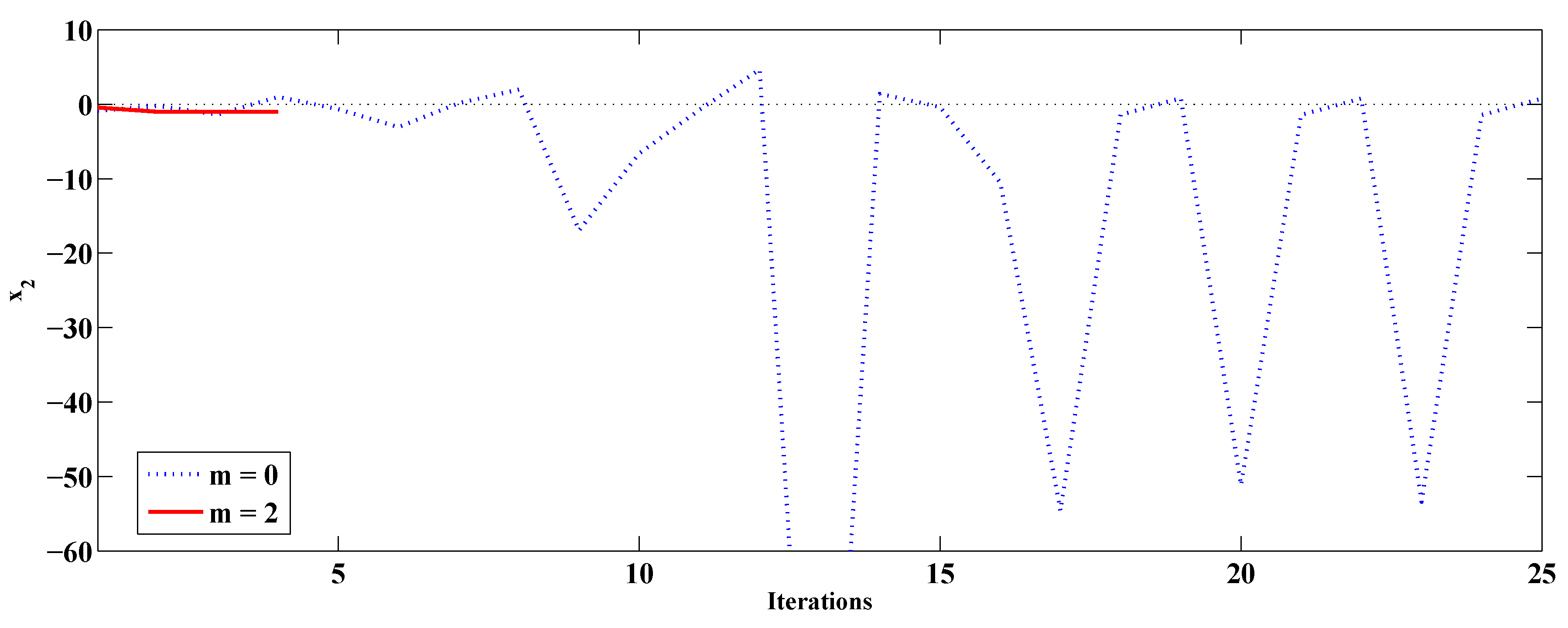
3.1. Negative Real Solutions

Let us assume that, as usually happens in engineering and science, one is mostly interested in finding the real solutions of nonlinear systems. Typically, for a particular application, it is known in advance whether the solutions will be positive or negative, according to the nature of the involved variables (e.g., in power engineering, voltage and current magnitudes are positive, by definition). As stated above, when those real solutions are positive, the factored method performs well. However, in the presence of negative solutions, some components of the auxiliary vector y will eventually become negative throughout the iterative process, driving the respective components of vector u to the complex domain (more specifically, to be of the form $u_k=ln|y_k|+\pi i$). In turn, when solving Equation (12) to obtain the log variables α (linear combinations of u variables), it may happen that one or several components ${\alpha }_k$ become also complex, with an angle other than π, which means that the original variable $x_k$ would be complex, rather than negative real. In those cases, the iterative process may remain oscillating or be diverted away from the basin of attraction of the intended real solution, eventually reaching one of the unsought complex solutions.

This potential risk is easily illustrated with the help of the following simple example.

example 1. Consider the solution of the system,

$$\begin{array}{ccc}\hfill p_1& =& x_1{x}_2+x_2\hfill \\ \hfill p_2& =& x_2^2+2x_1\hfill \end{array}$$

(13)

For $p_1=-10$ and $p_2=19$, there are two real solutions, $x=[3,-5]$ and $x=[9,-1]$, both of them containing a negative component. The two constant matrices involved in the factored procedure are in this case:

$$E=\left(\begin{array}{cccc}0& 1& 1& 0\\ 2& 0& 0& 1\end{array}\right);C=\left(\begin{array}{cc}1& 0\\ 0& 1\\ 1& 1\\ 0& 2\end{array}\right)$$

and the nonlinear transform, $u=f\left(y\right)$,

$$u=ln\left(\begin{array}{c}{y}_1\\ y_2\\ y_3\\ y_4\end{array}\right)\text{with}y=\left(\begin{array}{c}{x}_1\\ x_2\\ x_1{x}_2\\ x_2^2\end{array}\right)$$

Starting from $x^{\left(0\right)}=[0,0]$, the first iteration provides the following results:

$$y^{\left(1\right)}=\left(\begin{array}{c}7.6\\ -5\\ -5\\ 3.8\end{array}\right);u^{\left(1\right)}=\left(\begin{array}{c}2.0281\\ 1.6094+\pi i\\ 1.6094+\pi i\\ 1.3350\end{array}\right);x^{\left(1\right)}=\left(\begin{array}{c}-3.9872-6.9061i\\ -0.8853-1.5334i\end{array}\right)$$

As is clearly seen, the two negative components of y translate into complex components in the solution x, which are obtained as the exponential of linear combinations of u components. These complex components of x propagate through the iterative process until a steady-state cyclic pattern settles down or a complex solution is eventually reached (it is very unlikely that vector x becomes again real during the transient period).

The simplest way of preventing this risk (i.e., the factored method being unable to smoothly converge to negative real solutions) is by adding a sufficiently large positive offset, m, to all variables in x, or at least to those components in x that are clear candidates to become negative, so that the resulting transformed problem has only positive real solutions. This idea is applied below to the previous example.

example 2. Introducing new variables, $x_{o1}=x_1+m$ and $x_{o2}=x_2+m$, the original Equation system (13) becomes:

$$\begin{array}{ccc}\hfill p_1-m^2+m& =& x_{o1}{x}_{o2}-m{x}_{o1}+(1-m)x_{o2}\hfill \\ \hfill p_2-m^2+2m& =& x_{o2}^2+2x_{o1}-2m{x}_{o2}\hfill \end{array}$$

(14)

and the new matrix E,

$$E=\left(\begin{array}{cccc}-m& 1-m& 1& 0\\ 2& -2m& 0& 1\end{array}\right)$$

Starting again from $x^{\left(0\right)}=[0,0]$, the first iteration provides this time the following results:

$$y^{\left(1\right)}=\left(\begin{array}{c}7.1429\\ 0.0476\\ 2.3333\\ 4.9048\end{array}\right);u^{\left(1\right)}=\left(\begin{array}{c}1.9661\\ -3.0445\\ 0.8473\\ 1.5902\end{array}\right);x^{\left(1\right)}=\left(\begin{array}{c}7.5497\\ -0.4475\end{array}\right)$$

After just four iterations, the process converges to,

$$x_o^{\left(4\right)}=\left(\begin{array}{c}11.0000\\ 1.0000\end{array}\right);x^{\left(4\right)}=\left(\begin{array}{c}9.0000\\ -1.0000\end{array}\right)$$

Figure 1. Evolution of $x_2$ as iterations progress for the simple system of Examples 1 ($m=0$) and 2 ($m=2$).

Figure 1. Evolution of $x_2$ as iterations progress for the simple system of Examples 1 ($m=0$) and 2 ($m=2$).

Figure 1 represents the evolution of $x_2$ along the iterative process for $m=0$ (real part only) and $m=2$. In the first case (‘vanilla’ factored solution), the iterative process oscillates in the complex domain after nearly 20 iterations, whereas it converges in just four iterations to the correct real solution with $m=2$.

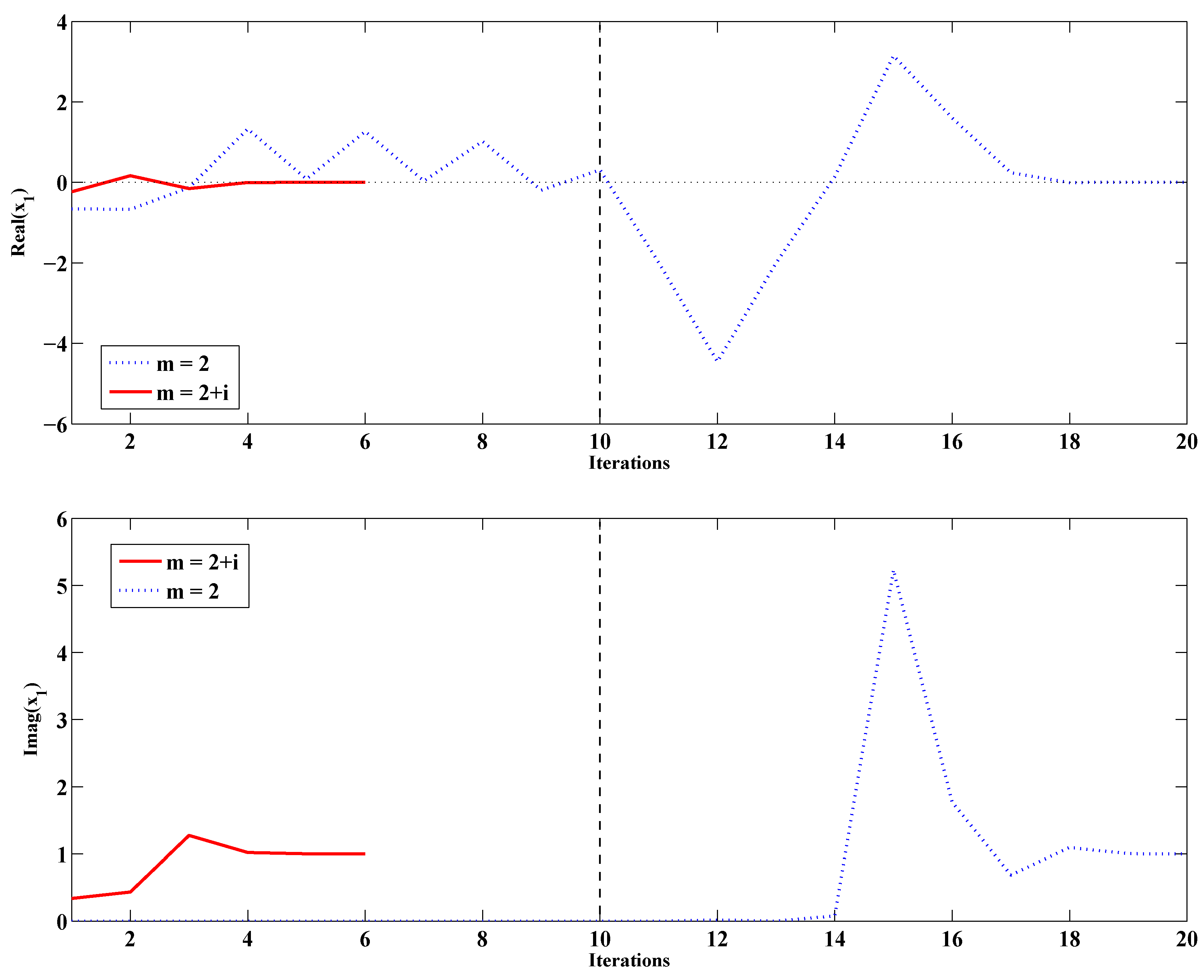
3.2. Complex Solutions

If the starting point does not lie in the basin of attraction of a real solution, or simply when real solutions do not exist at all, the factored iterative procedure is able to converge to a complex solution. However, as it is never known in advance whether the starting point is in the basin of a positive, negative or complex solution, it is advisable to always add a sufficiently large positive offset m, as discussed in the previous section. The problem of adding such a positive offset is that, when starting from a real starting point, the iterative process will not abandon the real domain unless a negative component arises by chance in y, which may not happen at all. This is a consequence of the log of a positive real number being also real. Fortunately, this problem is easily solved by adding an imaginary component to the offset m, as illustrated in the following example.

example 3. Consider again the simple system of the previous examples, but this time with $p_1=2$ and $p_2=0$, which has the real solution $x=[-2,-2]$ and the complex conjugate solution $x=[\pm i,1\pm i]$. Starting from $x^{\left(0\right)}=[0,0]$, with $m=2$, the values of $x_1$ and $x_2$ show initially a sustained oscillatory behavior (see Figure 2) until $x_1$ becomes negative at Iteration 9. Afterwards, the imaginary component of $x_1$ is non-null, and the iterative process manages to converge after 20 iterations to one of the complex conjugate solutions. For other starting points, the oscillations may persist much longer or indefinitely. However, with $m=2+i$, the factored method quickly converges in six iterations, as shown in Figure 2.

Figure 2. Evolution of real ($x_1$) and imag ($x_1$) as iterations progress for the simple system of Example 3 with $m=2$ and $m=2+i$.

Figure 2. Evolution of real ($x_1$) and imag ($x_1$) as iterations progress for the simple system of Example 3 with $m=2$ and $m=2+i$.

In summary, a positive real offset m is needed to prevent the iterative process from converging to complex solutions when searching for real negative solutions. Reciprocally, an imaginary component should be added to m so that complex solutions more easily pop up when real solutions do not exist or are of no interest.

4. Generalized Offset-Assisted Factored Solution

As discussed above, the idea is to prevent the appearance of negative variables by simply adding a sufficiently large scalar m to all components of the unknown vector, or at least those which are suspected to eventually become negative throughout the solution process, as follows:

$$x_o=x+m\left[\begin{array}{c}1\\ 1\\ ⋮\\ 1\end{array}\right]$$

(15)

Then, the original Equation system (1) is expressed in terms of the new set of positive variables,

$$h_o\left(x_o\right)=p_o$$

(16)

In turn, the resulting system can be factored in the same way as the original one, leading to the transformed system:

$$\begin{array}{ccc}\hfill E_{o}y& =& p_o\hfill \end{array}$$

(17)

$$\begin{array}{ccc}\hfill u& =& f_o\left(y\right)\hfill \end{array}$$

(18)

$$\begin{array}{ccc}\hfill C{x}_o& =& u\hfill \end{array}$$

(19)

which can be solved by applying the three-step procedure reviewed in Section 2 without facing the risk of negative variables arising.

Finally, the original variables x can be easily recovered by removing the offset m.

5. Case Studies

Two case studies will be used to compare the performance of the offset-assisted factored method with that of the standard Newton’s method.

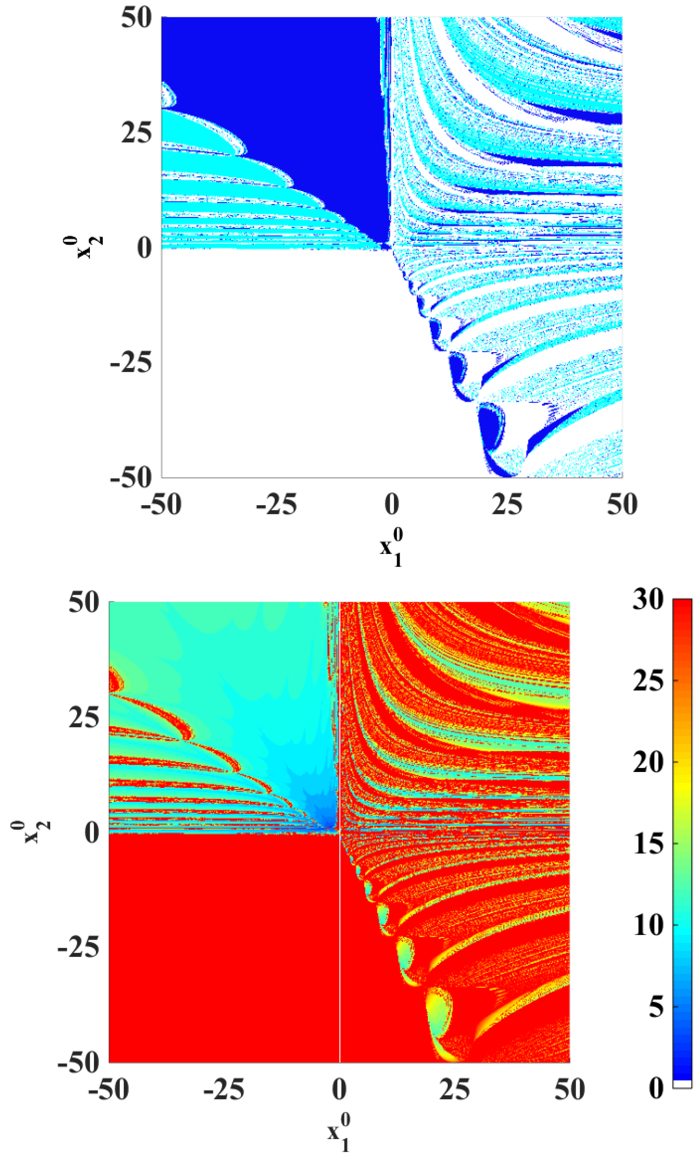
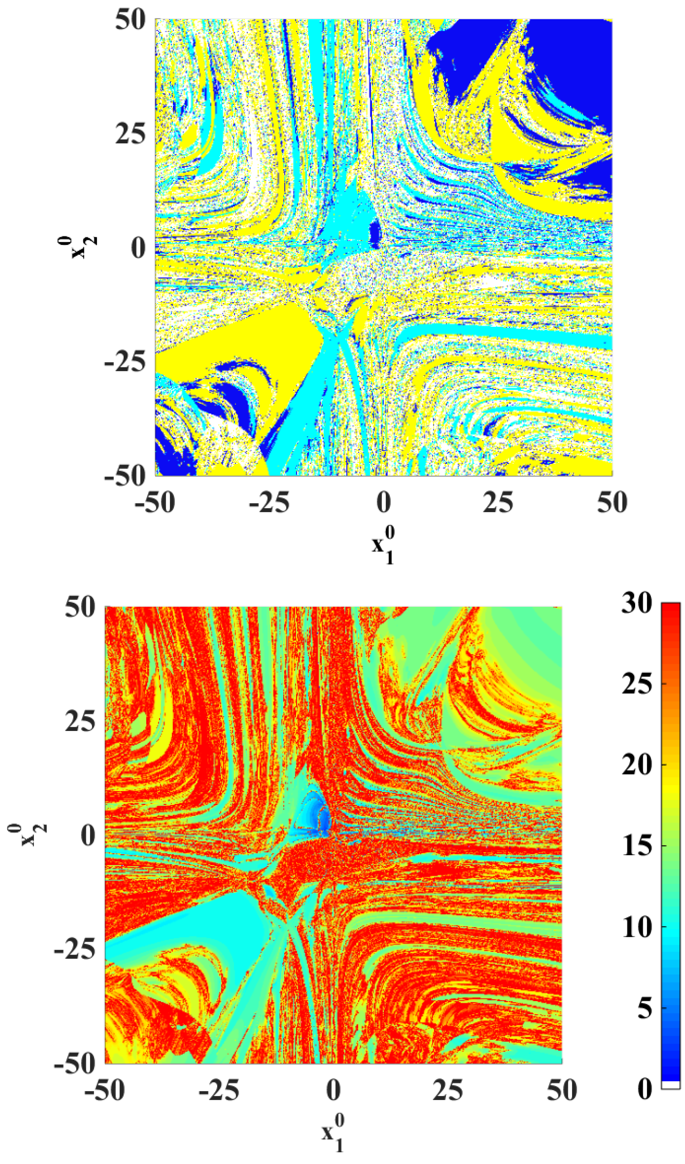
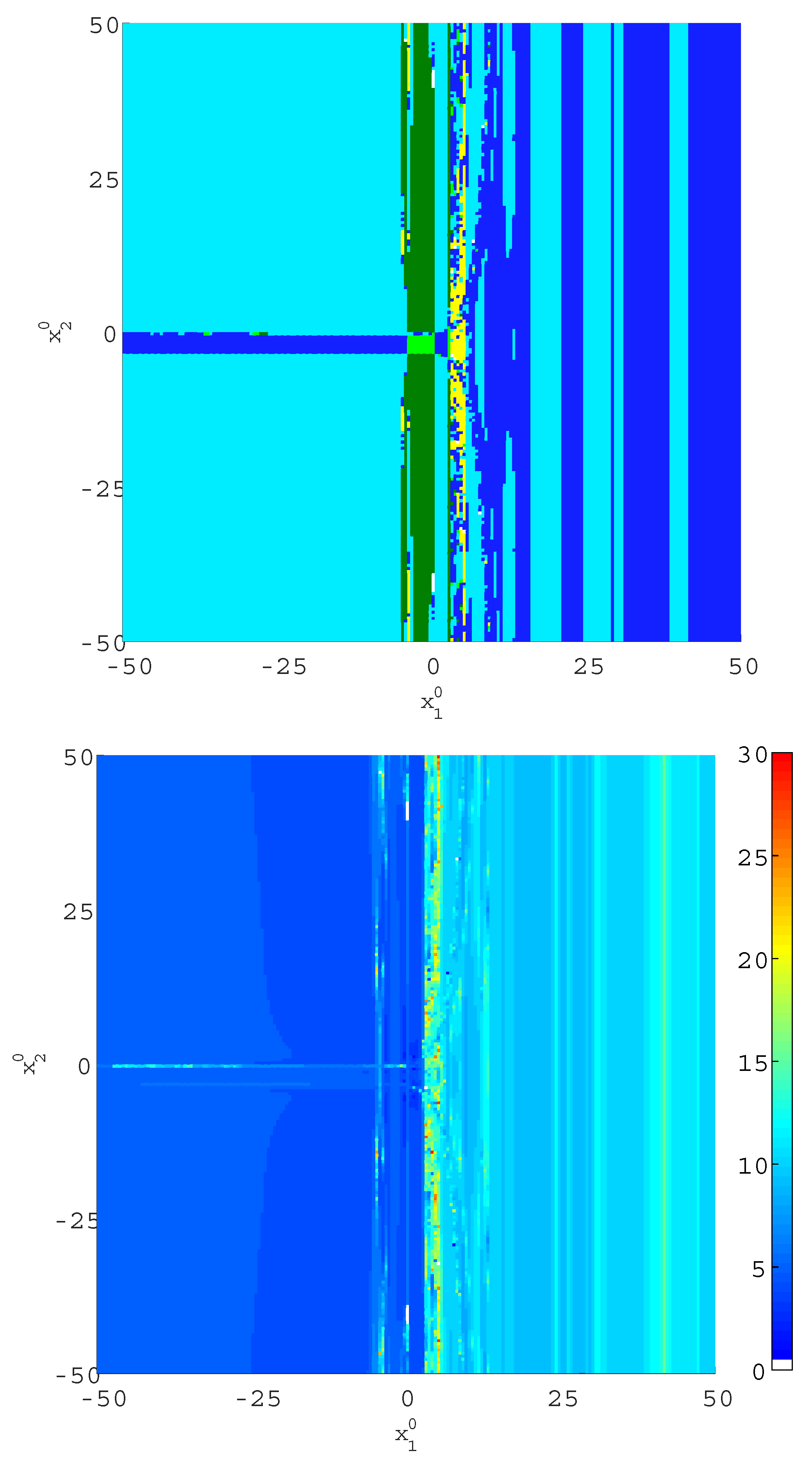
5.1. Fourth-Order Polynomial System

Consider the following 2 × 2 nonlinear system,

$$\begin{array}{ccc}\hfill p_1& =& x_1{x}_2^2\hfill \\ \hfill p_2& =& 2x_1^2{x}_2-x_1^2\hfill \end{array}$$

(20)

which is equivalent to two fourth-order polynomials in $x_1$ and $x_2$. For $p_1=-4$ and $p_2=4$, it is satisfied by the solutions shown in Table 1, two of them real with a negative component.

Table 1. Solutions of the 4th-order system for $p_1=-4$ and $p_2=4$.

$x_1$	$x_2$	Color
$-2$	1
$-3.8581$	0.6344
$0.2624\pm 0.7889$i	$-1.8172\pm 1.733$i
-	-

Table 1. Solutions of the 4th-order system for $p_1=-4$ and $p_2=4$.

$x_1$	$x_2$	Color
$-2$	1
$-3.8581$	0.6344
$0.2624\pm 0.7889$i	$-1.8172\pm 1.733$i
-	-

Figure 3 shows the basins of attraction (upper) and the number of iterations (lower) corresponding to Newton’s method. The colors corresponding to each solution are in accordance with those of Table 1, where the white color means that no convergence is achieved.

Figure 3. Basins of attraction (upper) and number of iterations (lower) for the fourth-order system when Newton’s method is applied.

Figure 3. Basins of attraction (upper) and number of iterations (lower) for the fourth-order system when Newton’s method is applied.

As can be noticed by the white color in the upper diagram (and the red color in the right one), when both components in $x_0$ are negative, convergence is never achieved. Moreover, many starting points in the first and fourth quadrant also lead to divergence. As expected, Newton’s method is not capable of reaching complex solutions (yellow color missing in the upper diagram).

Figure 4 is the counterpart of Figure 3 for the factored method with a real offset ($m=10$). As can be seen, in the neighborhood of the two real solutions (central area in the diagrams), the behavior of the factored method is similar to that of Newton’s method. However, the total surface of the white areas in the upper diagram (non-convergent cases) is much smaller than that of Figure 3, indicating lower risk of divergence when using the factored method.

Figure 4. Basins of attraction (upper) and number of iterations (lower) for the fourth-order system when the factored method with $m=10$ is applied.

Figure 4. Basins of attraction (upper) and number of iterations (lower) for the fourth-order system when the factored method with $m=10$ is applied.

Finally, the results obtained with the factored method with $m=10+5i$ are shown in Figure 5. Compared to Figure 4, it is clear that white areas in the upper diagram have virtually faded away (no risk of divergence at all), while convergence to real solutions in their neighborhood (central area in light and dark blue) is preserved. Large areas in yellow are also apparent in the upper diagram, indicating that the addition of an imaginary component to m clearly favors the trend to reach complex solutions.

Figure 5. Basins of attraction (upper) and number of iterations (lower) for the fourth-order system when the factored method with $m=10+5i$ is applied.

Figure 5. Basins of attraction (upper) and number of iterations (lower) for the fourth-order system when the factored method with $m=10+5i$ is applied.

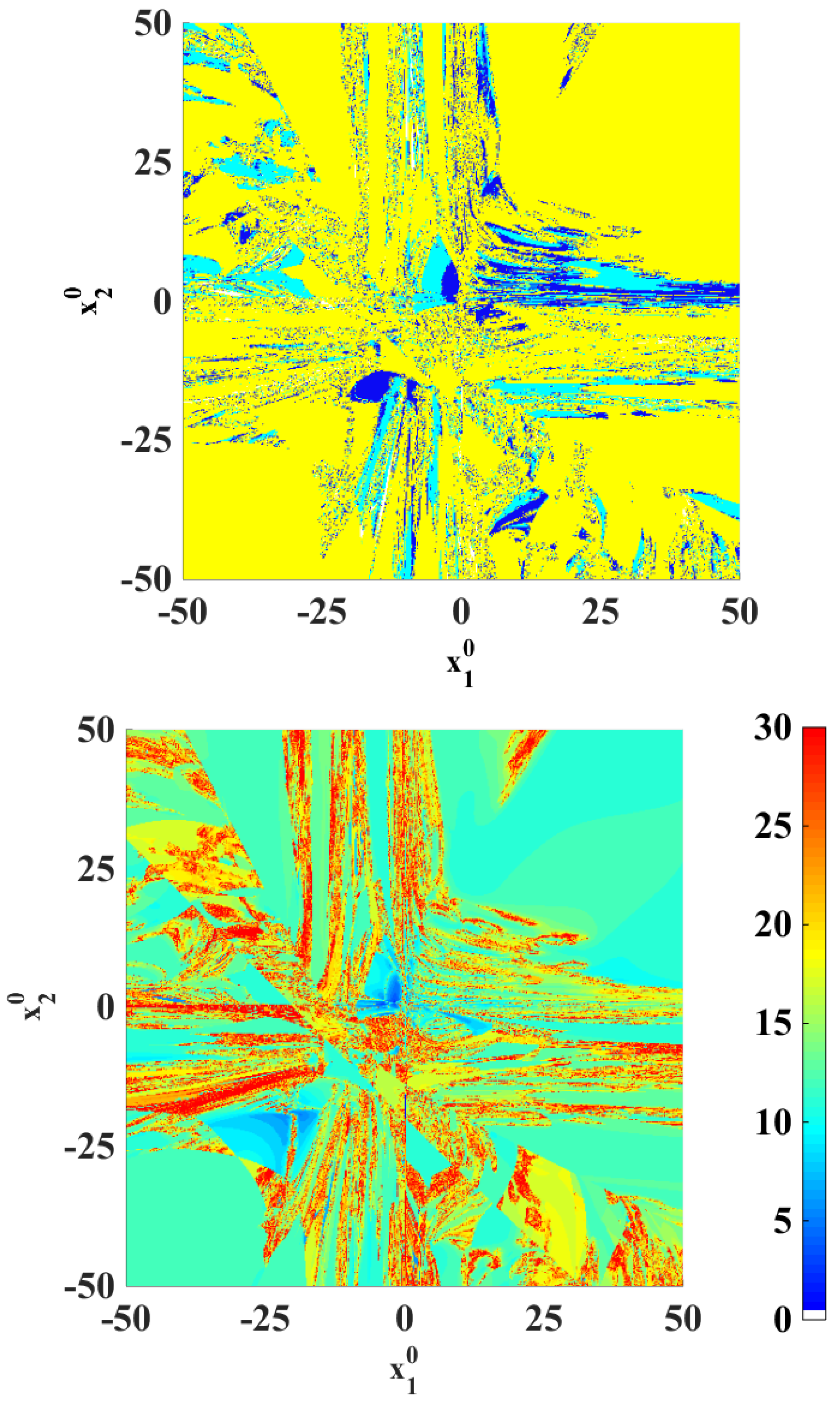
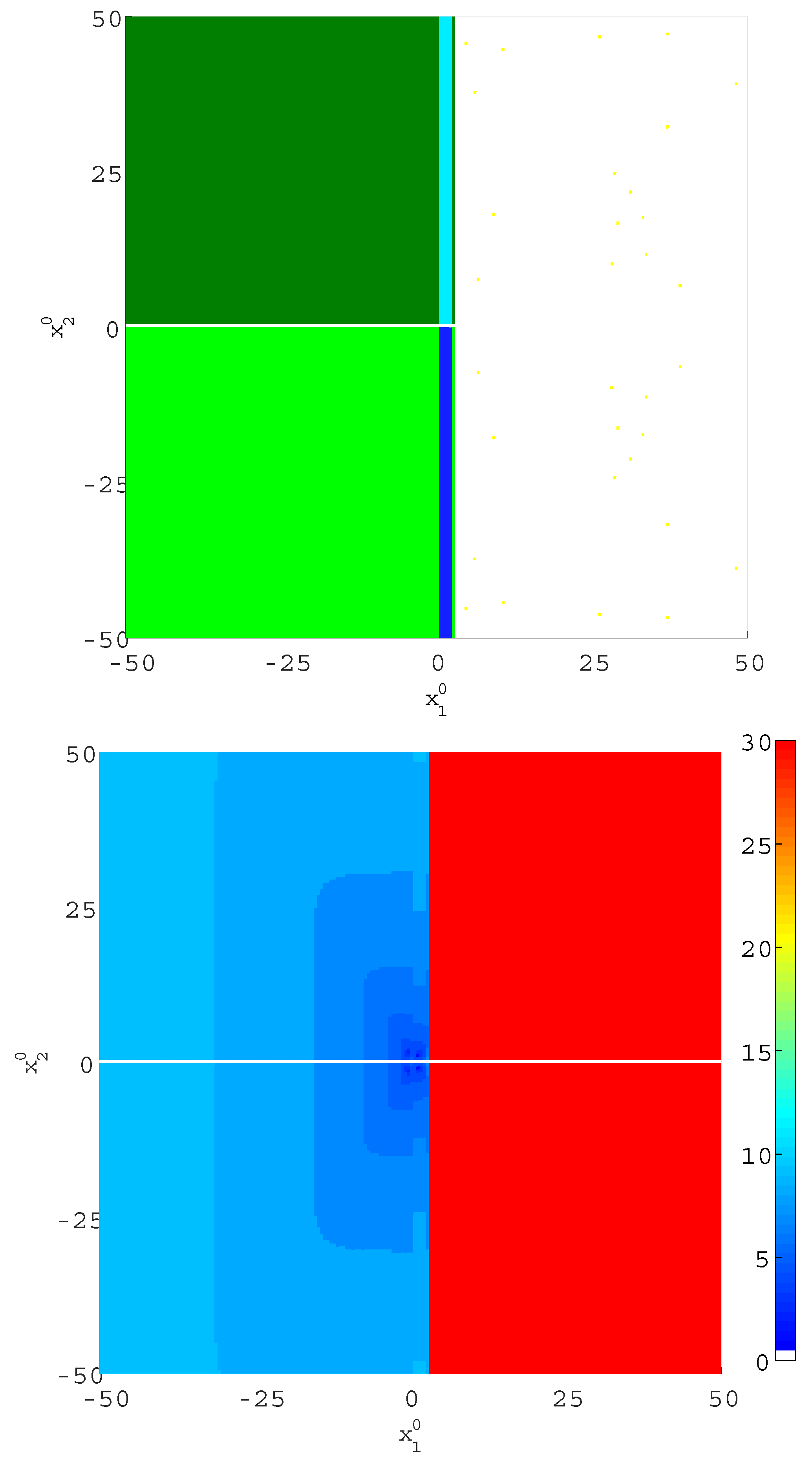
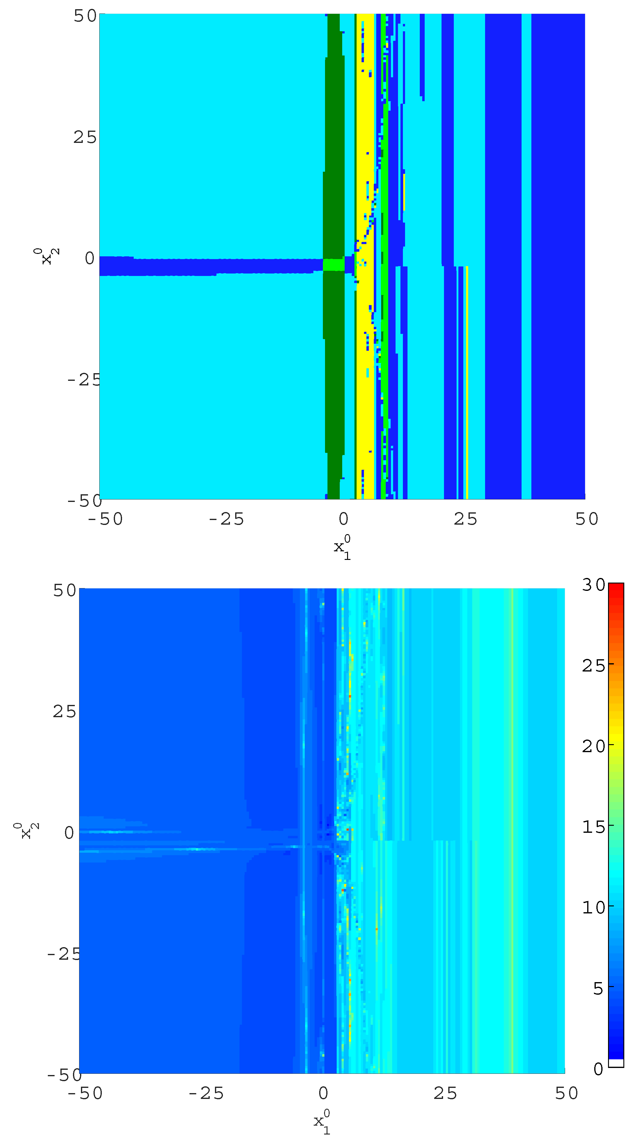
5.2. Kelley’s Synthetic System

The next system studied, originally posed by Kelley [12], is as follows:

$$\begin{array}{ccc}\hfill 2& =& x_1^2+x_2^2\hfill \\ \hfill 2& =& e^{x_1-1}+x_2^2\hfill \end{array}$$

(21)

This system is symmetric under the transformation $x_2\to -x_2$ and has the solutions provided in Table 2.

Figure 6 shows the basins of attraction (upper) and number of iterations (lower) corresponding to Newton’s method. The colors corresponding to each solution are in accordance with those of Table 2, where the white color means that no convergence is achieved. In this apparently simple case, the basins of attraction are perfect rectangles, and convergence is not possible in most of the right half plane. Since the Jacobian is singular along the line $x_2=0$, Newton’s method gets in trouble also in that region.

Table 2. Solutions for Kelley’s system.

$x_1$	$x_2$	Color
1	$-1$
1	1
$-0.4777$	$-1.3311$
$-0.4777$	1.3311
3.5129	$-3.2156i$
-	-

Table 2. Solutions for Kelley’s system.

$x_1$	$x_2$	Color
1	$-1$
1	1
$-0.4777$	$-1.3311$
$-0.4777$	1.3311
3.5129	$-3.2156i$
-	-

Figure 6. Basins of attraction (upper) and number of iterations (lower) for Kelley’s system when Newton’s method is applied.

Figure 6. Basins of attraction (upper) and number of iterations (lower) for Kelley’s system when Newton’s method is applied.

Figure 7 is the counterpart of Figure 6 for the factored method with a real offset ($m=2$). As can be seen, the white (red) color in the upper (lower) diagram has vanished, which means that convergence is achieved nearly globally. The symmetry around $x_2$ is still apparent.

Figure 7. Basins of attraction (upper) and number of iterations (lower) for Kelley’s system when the factored method with $m=2$ is applied.

Figure 7. Basins of attraction (upper) and number of iterations (lower) for Kelley’s system when the factored method with $m=2$ is applied.

Finally, the results obtained with the factored method with $m=10+0.5i$ are shown in Figure 8. Compared to Figure 7, a larger and more homogenous yellow area is visible in the central part of the left diagram, indicating the trend for the factored method to reach complex solutions when m has an imaginary component, as explained in Section 3.2.

Figure 8. Basins of attraction (upper) and number of iterations (lower) for Kelley’s system when the factored method with $m=2+0.5i$ is applied.

Figure 8. Basins of attraction (upper) and number of iterations (lower) for Kelley’s system when the factored method with $m=2+0.5i$ is applied.

6. Conclusions

This paper has addressed the difficulties faced by the factored solution method when solving nonlinear systems with negative or complex solutions. It has been shown that by adding a sufficiently large real offset, both positive and negative real solutions can be safely reached. Moreover, if no real solutions exist or the user is rather interested in finding complex solutions, it is advisable to add an imaginary component to the offset. Some examples have been worked out showing that, while locally preserving the quadratic convergence rate of Newton’s method, the global behavior (basins of attractions) of the factored procedure can be tuned to a large extent with the help of the proposed offset, increasing the chances for real or complex solutions to be selectively reached.

References

1. Kuo, M. Solution of nonlinear equations. IEEE Trans. Comput. 1968, 17, 897–898. [Google Scholar] [CrossRef]
2. Rice, J. Numerical Methods, Software, and Analysis; Academic Press: New York, NY, USA, 1993. [Google Scholar]
3. Ortega, J.M.; Rheinboldt, W.C. Iterative Solution of Nonlinear Equations in Several Variables; Academic Press: New York, NY, USA, 1970; (also published by SIAM, Philadelphia, 2000). [Google Scholar]
4. Kelley, C.T. Iterative Methods for Linear and Nonlinear Equations; SIAM: Philadelphia, PA, USA, 1995. [Google Scholar]
5. Deuflhard, P. Newton Methods for Nonlinear Problems; Springer-Verlag: Heidelberg, Germany, 2004. [Google Scholar]
6. Kelley, C.T. Solving Nonlinear Equations with Newton’s Method, Fundamentals of Algorithms; SIAM: Philadelphia, PA, USA, 2003. [Google Scholar]
7. Judd, K.L. Numerical Methods in Economics; MIT Press: Boston, MA, USA, 1998. [Google Scholar]
8. Gómez-Expósito, A. Factored Solution of Nonlinear Equation Systems. Proc. R. Soc. A 2014. [Google Scholar] [CrossRef]
9. Gómez-Expósito, A.; Gómez-Quiles, C. Factorized Load Flow. IEEE Trans. Power Syst. 2013, 28, 4607–4614. [Google Scholar] [CrossRef]
10. Gómez-Expósito, A.; Gómez-Quiles, C.; Vargas, W. Factored Solution of Infeasible Load Flow Cases. In Proceedings of the Power Systems Computation Conference (PSCC), Wroclaw, Poland, 18–22 August 2014.
11. Sandberg, I.W.; Willson, A.N. Existence and Uniqueness of Solutions for the Equations of Nonlinear DC Networks. SIAM J. Appl. Math. 1972, 22, 173–186. [Google Scholar] [CrossRef]
12. Rheinboldt, W. Some Nonlinear Test Problems. Available online: http://folk.uib.no/ssu029/Pdf_file/Testproblems/testprobRheinboldt03.pdf (accessed on 22 December 2015).