1. Introduction
The function optimization problem is to find the optimal solution of the objective function by the iterative [
1]. In general, the search objective is to optimize the function of the objective function, which is usually described by the continuous, discrete, linear, nonlinear, concave and convex of the function. For constrained optimization problems, one can adopt the specific operators to make the solutions always feasible, or use the penalty function to transform the solutions into the unconstrained problems. So, the unconstrained optimization problems are the research focus here. There has been considerable attention paid to employing metaheuristic algorithms inspired from natural processes and/or events in order to solve function optimization problems. The swarm intelligent optimization algorithm [
2] is a random search algorithm simulating the evolution of biological populations. It can solve complex global optimization problems through the cooperation and competition among individuals. The representative swarm intelligence optimization algorithms include Ant Colony Optimization (ACO) algorithm [
3], Genetic Algorithm (GA) [
4], Particle Swarm Optimization (PSO) algorithm [
5], Artificial Bee Colony (ABC) algorithm [
6],
etc.However, not all met heuristic algorithms are bio-inspired, because their sources of inspiration often come from physics and chemistry. For the algorithms that are not bio-inspired, most have been developed by mimicking certain physical and/or chemical laws, including electrical charges, gravity, river systems,
etc. The typical physics and chemistry inspired met heuristic algorithms include Big Bang-big Crunch optimization algorithm [
7], Black hole algorithm [
8], Central force optimization algorithm [
9], Charged system search algorithm [
10], Electro-magnetism optimization algorithm [
11], Galaxy-based search algorithm [
12], Harmony search algorithm [
13], Intelligent water drop algorithm [
14], River formation dynamics algorithm [
15], Self-propelled particles algorithm [
16], Spiral optimization algorithm [
17], Water cycle algorithm [
18],
etc.The gravitational search algorithm (GSA) was introduced by E. Rashedi
et al. in 2009 [
19]. It was constructed based on the law of gravity and the notion of mass interactions. The GSA algorithm uses the theory of Newtonian physics and its searcher agents are the collection of masses. A multi-objective gravitational search algorithm (MOGSA) technique was proposed to be applied in hybrid laminates to achieve minimum weight and cost [
20]. A fuzzy gravitational search algorithm was proposed for a pattern recognition application, which in addition provided a comparison with the original gravitational approach [
21]. The grouping GSA (GGSA) adapted the structure of GSA for solving the data clustering problem [
22]. Combining the advantages of the gravitational search algorithm (GSA) and gauss pseudo spectral method (GPM), an improved GSA (IGSA) is presented to enhance the convergence speed and the global search ability [
23]. A novel modified hybrid Particle Swarm Optimization (PSO) and GSA based on fuzzy logic (FL) was proposed to control the ability to search for the global optimum and increase the performance of the hybrid PSO-GSA [
24]. A binary quantum-inspired gravitational search algorithm (BQIGSA) was proposed by using the principles of QC together with the main structure of GSA to present a robust optimization tool to solve binary encoded problems [
25]. Another binary version of hybrid PSOGSA called BPSOGSA was proposed to solve many kinds of optimization problems [
26]. A new gravitational search algorithm was proposed to solve the unit commitment (UC) problem, which is the integrated binary gravitational search algorithm (BGSA) with the Lambda-iteration method [
27].
In conclusion, GSA has been successfully applied in many global optimization problems, such as, multi-objective optimization of synthesis gas production [
28], the forecasting of turbine heat rate [
29], dynamic constrained optimization with offspring repair [
30], fuzzy control system [
31], grey nonlinear constrained programming problem [
32], reactive power dispatch of power systems [
33], minimum ratio traveling salesman problem [
34], parameter identification of AVR system [
35], strategic bidding [
36],
etc. In this paper, the research on the function optimization problem is solved based on the gravitation search algorithm (GSA). Then the parameter performance comparison and analysis are carried out through the simulation experiments in order to verify its superiority. The paper is organized as follows. In
Section 2, the gravitational search algorithm is introduced. The simulation experiments and results analysis are introduced in details in
Section 3. Finally, the conclusion illustrates the last part.
2. Gravitational Search Algorithm
2.1. Physics Foundation of GSA
The law of universal gravitation is one of the four basic forces in nature. It is one of the fundamental forces in nature. The gravitational force is proportional to the product of the mass, and is inversely proportional to the square of the distance. The gravitational force between two objects is calculated by:
where,
is the gravitational force between two objects,
is the gravitational constant,
and
are the masses of the objects 1 and 2 respectively,
is the distance between these two objects. According to the international unit system, the unit of
is Newton (N), the unit of
and
is kg, the unit of
is m, and the constant
is approximately equal to
.
The acceleration of the particle
is related to its mass
and of the gravitational force
, which is calculated by the following equation.
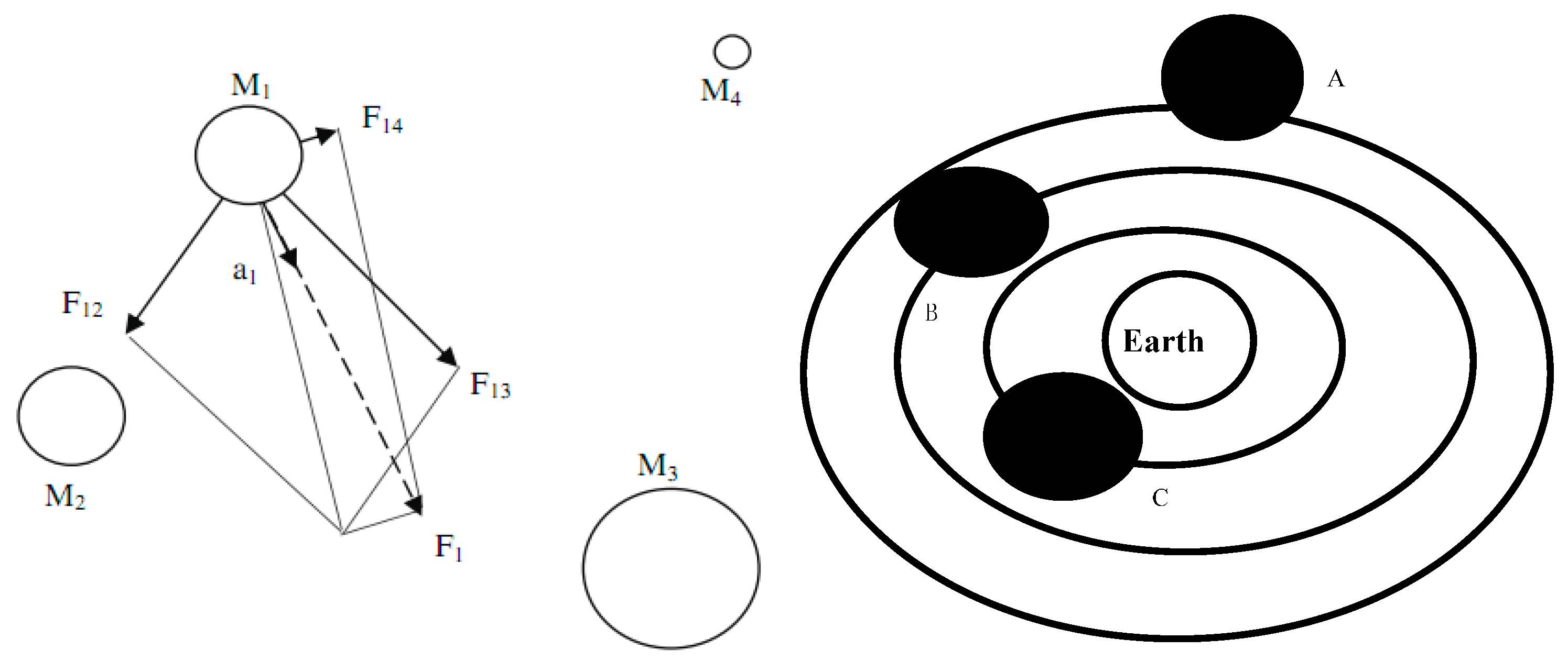
According to the Equations (1) and (2), all of the particles in the world are affected by gravity. The closer the distance between two particles, the greater the gravitational force. Its basic principle is shown in
Figure 1, where the mass of the particles is represented by the image size. Particle
is influenced by the gravity of the other three particles to produce the resultant force
. Such an algorithm will converge to the optimal solution, and the gravitational force will not be affected by the environment, so the gravity has a strong local value.
Figure 1.
Gravitational phenomena.
Figure 1.
Gravitational phenomena.
The gravitational search algorithm should make the moving particle in space into an object with a certain mass. These objects are attracted through gravitational interaction between each other, and each particle in the space will be attracted by the mutual attraction of particles to produce accelerations. Each particle is attracted by the other particles and moves in the direction of the force. The particles with small mass move to the particles with great mass, so the optimal solution is obtained by using the large particles. The gravitation search algorithm can realize the information transmission through the interaction between particles.
2.2. Basic Principles of Gravitation Search Algorithm
Because there is no need to consider the environmental impact, the position of a particle is initialized as . Then in the case of the gravitational interaction between the particles, the gravitational and inertial forces are calculated. This involves continuously updating the location of the objects and obtaining the optimal value based on the above mentioned algorithm. The basic principal of gravitational search algorithm is described as follows in detail.
2.2.1. Initialize the Locations
Firstly, randomly generate the positions
of
objects, and then the positions of
objects are brought into the function, where the position of the
th object are defined as follows.
2.2.2. Calculate the Inertia Mass
Each particle with certain mass has inertia. The greater the mass, the greater the inertia. The inertia mass of the particles is related to the self-adaptation degree according to its position. So the inertia mass can be calculated according to the self-adaptation degree. The bigger the inertial mass, the greater the attraction. This point means that the optimal solution can be obtained. At the moment
, the mass of the particle
is represented as
. Mass
can be calculated by the followed equation.
where
,
is the fitness value of the object
,
is the optimal solution and
is the worst solution. The calculation equation of
and
are described as follows.
For solving the maximum problem:
For solving the minimum value problem:
2.2.3. Calculate Gravitational Force
At the moment
, the calculation formula for the gravitational force of object
to object
described as follows.
where,
is a very small constant,
is the inertial mass of the object itself,
is the inertial mass of an object
.
is the universal gravitational constant at the moment
, which is determined by the age of the universe. The greater the age of the universe, the smaller
. The inner relationship is described as follows.
where
is the universal gravitational constant of the universe at the initial time
, generally it is set as 100.
is 20,
is the maximum number of iterations and
represented the Euclidean distance between object
and object
.
In GSA, the sum
of the forces acting on the
in the
-th dimension is equal to the sum of all the forces acting on this object:
where
is the random number in the range
,
is the gravity of the
-th object acting on the
the object in the
-th dimension space. According to Newton's Second Law, the acceleration of the
-th particle in the
-th dimension at the moment
is defined as follows:
2.2.4. Change the Positions
In each iteration, the object position can be changed by calculating the acceleration, which is calculated by the following equations.
2.3. Algorithm Flowchart
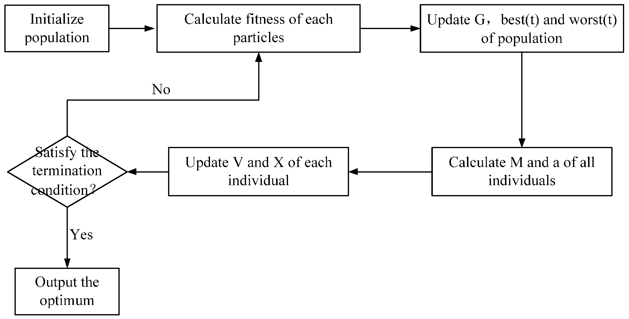
The detailed flowchart of the algorithm is shown in
Figure 2, and the optimization procedure is described as follows.
Figure 2.
Flowchart of gravitational search algorithm (GSA).
Figure 2.
Flowchart of gravitational search algorithm (GSA).
Step 1: Initialize the positions and accelerations of all particles, the number of iterations and the parameters of the GSA;
Step 2: According to the Equation (12), calculate the fitness value of each particle and update the gravity constant;
Step 3: According to the Equations (5)–(7), calculate the quality of the particles based on the obtained fitness values and the acceleration of each particle according to the Equations (8) and (15);
Step 4: Calculate the velocity of each particle and update the position of the particle according to the Equation (17);
Step 5: If the termination condition is not satisfied, turn to Step 2, otherwise output the optimal solution.
2.4. Analysis of Gravitational Search Algorithm
In GSA, the update of the particle positions is aroused by the acceleration caused by the gravitational force of the particles. The value of gravity determines the size of the particle’s acceleration, so the acceleration can be regarded as the search step of the particle position update. Its size determines the convergence rate of the gravitational search algorithm. In the acceleration calculation, the number of particles and gravity play an important role, and the mass and gravity of the particles are determined the variety of . The particle with different mass and gravity has different convergence rate. So it is very important to choose the number of particles and the gravity of the universal gravitation search algorithm.
The parameter initialization for all swarm intelligence optimization algorithms has important influence on the performance of the algorithms and the optimization ability. GSA has two main steps: one is to calculate the attraction of other particles for their selves and the corresponding acceleration calculated through gravitational, and another is to update the position of the particles according to the calculated acceleration. As shown in Formula (11)–(17), the convergence rate of GSA is determined by the value of Gravitational constant to determine the size of the particle acceleration, and parameters to determine the pace of change. In this section, the effect and influence of parameters and will be analyzed in detail.
3. Simulation Experiments and Results Analysis
3.1. Test Functions
Six typical functions shown in
Table 1 are selected and carried out simulation experiments for the optimal solution under the condition of GSA changeable parameters. There is only one extreme point for
, which is mainly used to investigate the convergence of the algorithm and to test the accuracy of the algorithm. There are many extreme points for
, the difference are in that
has lower dimension 2 and 4 respectively, while
are high dimension with 30.
Table 1.
Typical test functions.
Table 1.
Typical test functions.
| Function | Name | Expression | Range | Dim |
|---|
| Griewank | | [−32, 32]n | 30 |
| Quartic | | [−1.28, 1.28]n | 30 |
| Rastrigin | | [−5.12, 5.12]n | 30 |
| Schwefel | | [−600, 600]n | 30 |
| Shekel’s Foxholes | | [−65.53, 65.53]2 | 2 |
| Kowalik’s | | [−5, 5]4 | 4 |
3.2. Simulation Results and Corresponding Analysis
The GSA parameters are initialized as follows: max iterations max_it = 1000, objects N = 100. When the simulation experiments are carried out for the parameters
,
= 20. In order to reduce the influence of random disturbance, the independent operation 50 times is carried out for each test function. The optimum values and average values of GSA under different
are shown in
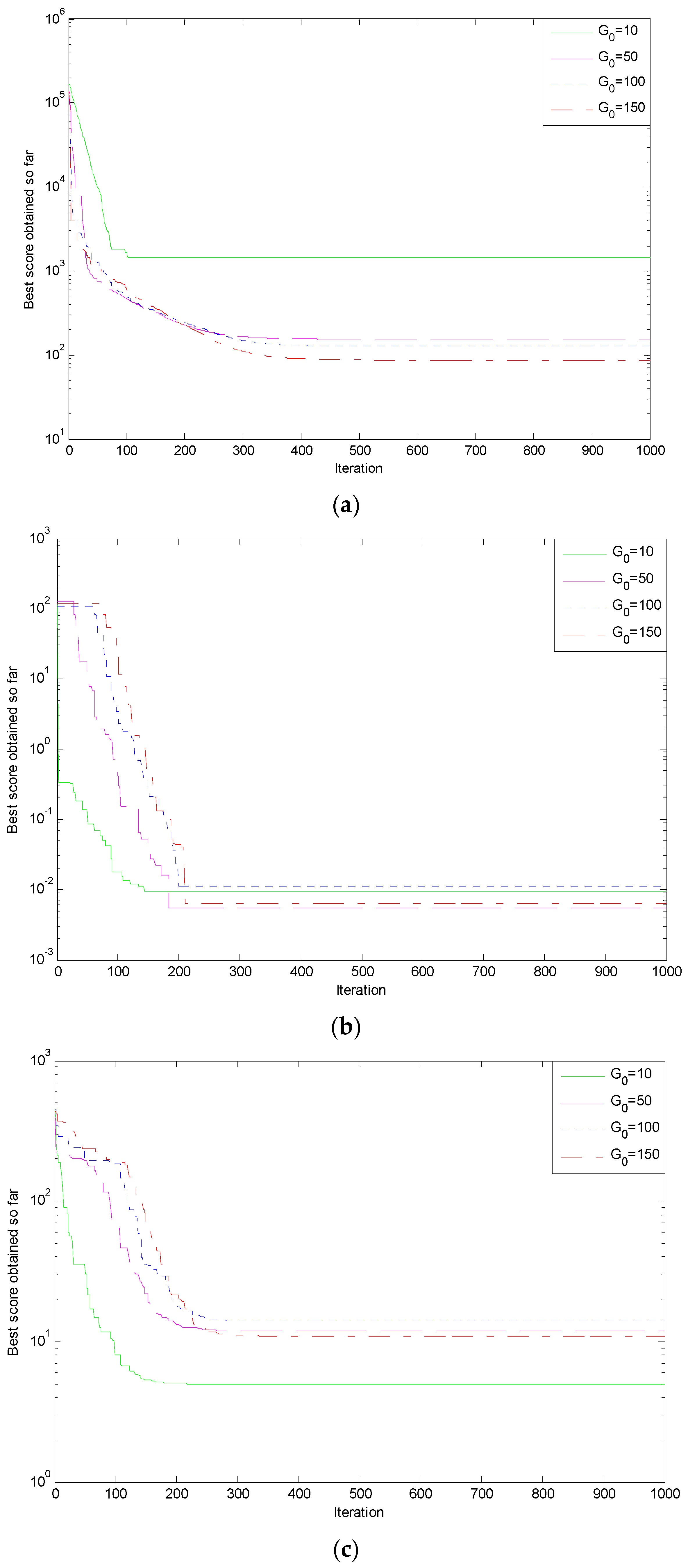
Table 2. The simulation curves for six test functions are shown in
Figure 3a–f.
Table 2.
The simulation result of different number of .
Table 2.
The simulation result of different number of .
| Function | Result | The Simulation Results of GSA under Different |
|---|
| 10 | 50 | 100 | 150 | Minimum Time (s) |
|---|
| optimum | 1.4465e+3 | 153.1636 | 127.7572 | 86.9076 | 9.1665 |
| average | 216.2229 | 210.4132 | 640.4764 | 1.0409e+4 |
| optimum | 0.0092 | 0.0055 | 0.0059 | 0.0062 | 7.6812 |
| average | 69.0872 | 101.8753 | 102.9537 | 78.0762 |
| optimum | 4.9748 | 11.9395 | 13.9294 | 10.9445 | 7.4739 |
| average | 236.9825 | 392.0198 | 367.3913 | 365.4881 |
| optimum | 315.2694 | 7.6050 | 2.4267 | 0.0123 | 7.7866 |
| average | 31.1370 | 0 | 0 | 0 |
| optimum | 1.0012 | 1.0909 | 1.0602 | 0.9980 | 7.3759 |
| average | 2.0043 | 0.9980 | 1.0836 | 1.4385 |
| optimum | 0.0013 | 0.0015 | 0.0017 | 0.0016 | 3.8364 |
| average | 0.0072 | 0.0106 | 0.096 | 0.0049 |
Figure 3.
Simulation results of six typical test functions. (a) Griewank function; (b) Quartic function; (c) Rastrigin function; (d) Schwefel function; (e) Shekel’s Foxholes function; (f) Kowalik’s oxholes function.
Figure 3.
Simulation results of six typical test functions. (a) Griewank function; (b) Quartic function; (c) Rastrigin function; (d) Schwefel function; (e) Shekel’s Foxholes function; (f) Kowalik’s oxholes function.
Seen from the above simulation results, when is 150, whether the optimal value or average value, the functions (, , ) all have achieved the best results. When are 100 and 50, the optimization effect decreased successively. When is 10, the functions (, , ) have the best convergence performance. However, the most obvious performance of convergence curves appears in the function and the curves of optimization effect in function and is worst. The parameter selection of different simulation curve fluctuates greatly in , where the simulation curves of the difference maximum when is 10 compared with other values. By analyzing the convergence curves of each function, the convergence rate of the low dimensional function was higher than the high dimensional function. Seen from the overall trends, as the growth of the value , the precision of solution obtained in the related function optimization is not growth, but it is affected by the optimal solution of distribution from the solution space of a different function. Moreover, it is also related to the size of the solution space.
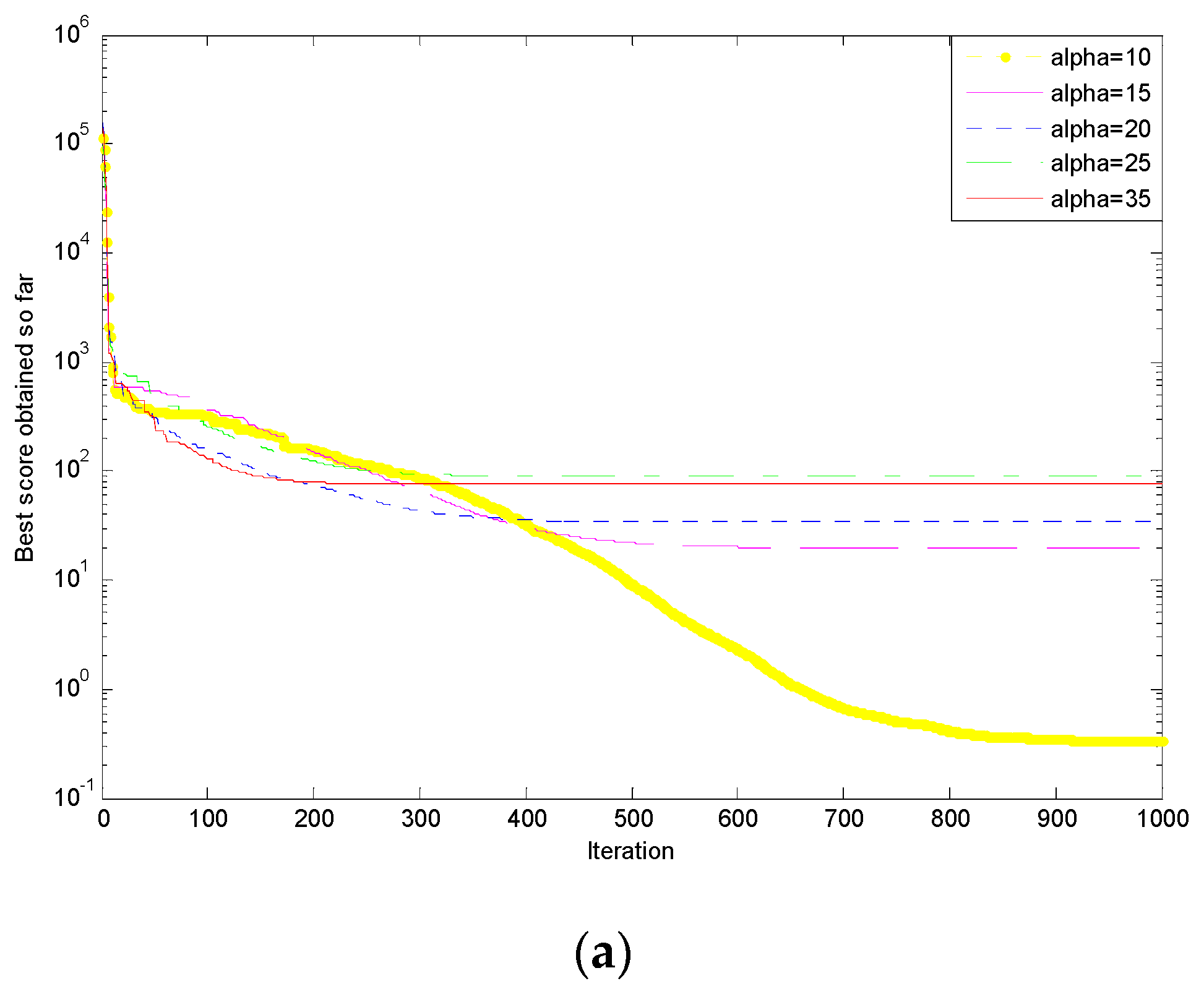
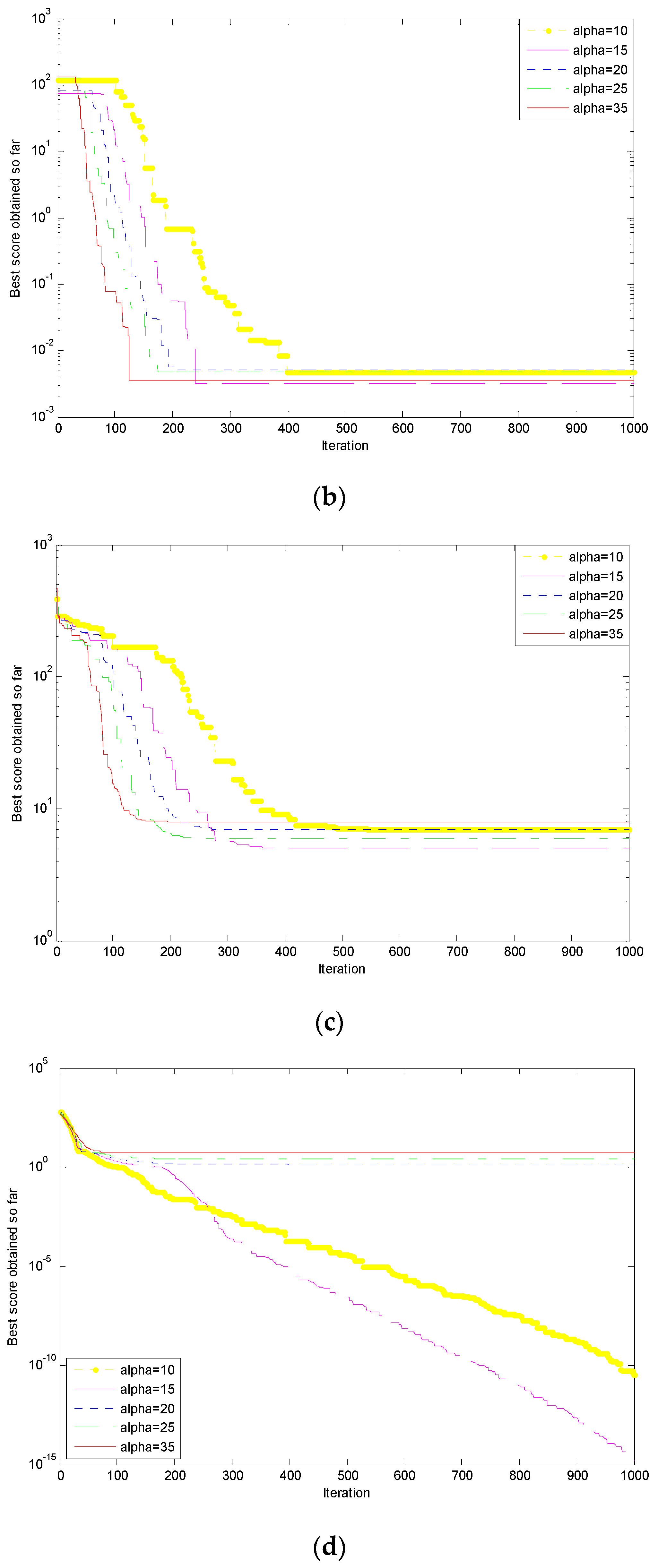
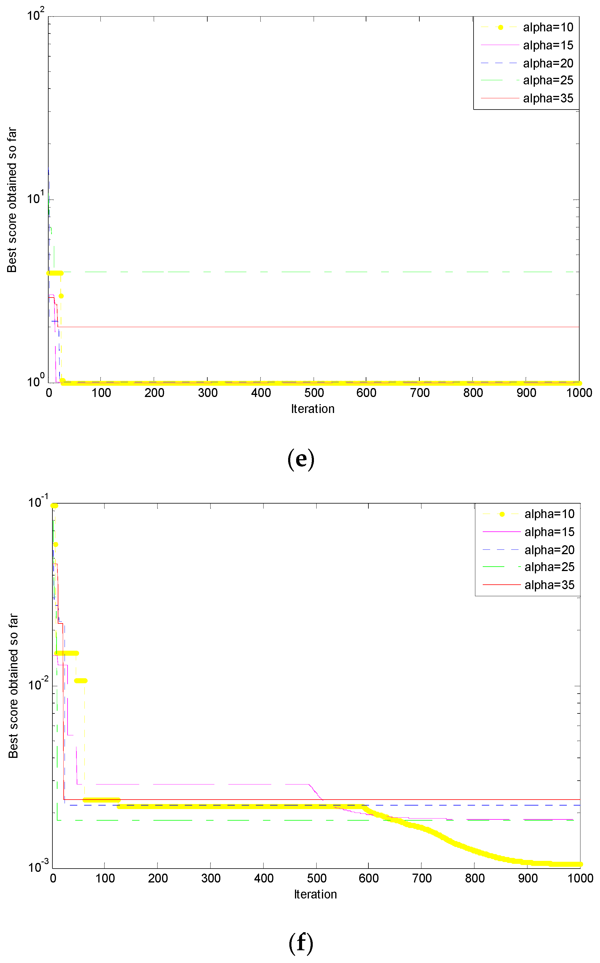
In view of the different values of the parameter
, the maximum or the minimum impact on the performance of function optimization are all varying. Considering the running time, the parameter
is 100 and the other parameters remain unchanged. The simulation experiments and the corresponding analysis for
are shown in
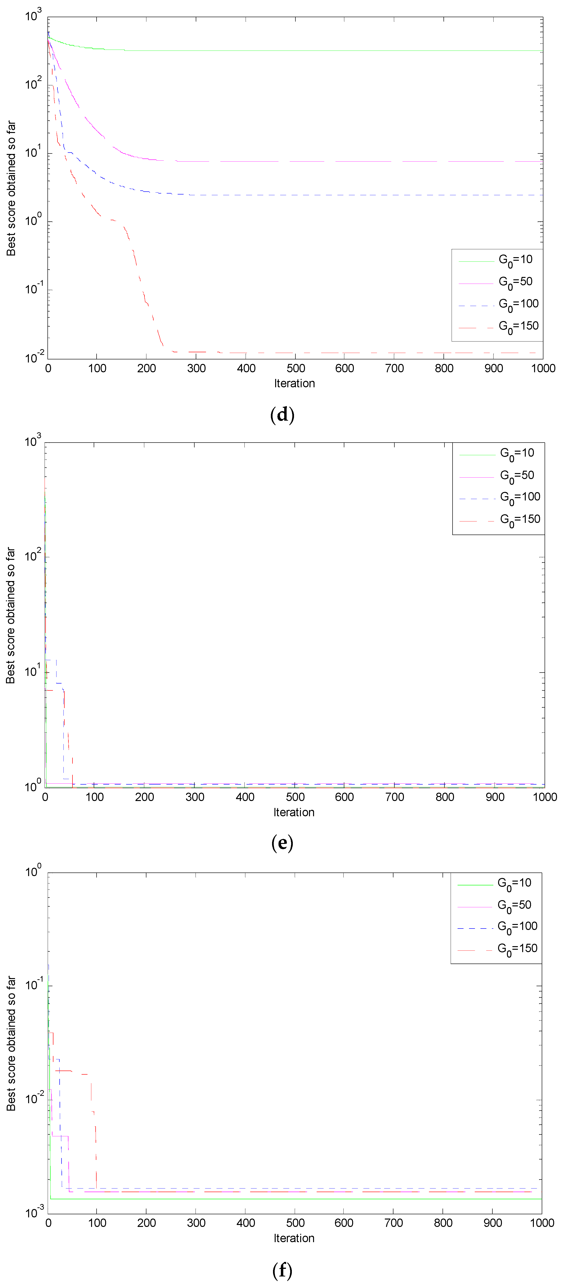
Table 3. The simulation curves of six test functions are shown in
Figure 4a–f.
Table 3.
The simulation result of different .
Table 3.
The simulation result of different .
| Function | The Simulation Results of GSA under Different |
|---|
| 10 | 15 | 20 | 25 | 35 | Minimum Time (s) |
|---|
| 0.3386 | 19.7209 | 34.1272 | 89.9338 | 75.9954 | 31.9325 |
| 0.0047 | 0.0033 | 0.0050 | 0.0048 | 0.0036 | 27.9789 |
| 6.9647 | 4.9748 | 6.9647 | 5.9698 | 7.9597 | 27.9227 |
| 3.2581e−11 | 1.5543e−15 | 1.3438 | 2.5285 | 5.3956 | 28.4755 |
| 0.9980 | 0.9980 | 1.0064 | 3.9684 | 2.0038 | 19.3953 |
| 0.0011 | 0.0019 | 0.0022 | 0.0018 | 0.0024 | 13.9513 |
Figure 4.
Simulation results of six typical test functions. (a) Griewank function ; (b) Quartic function ; (c) Rastrigin function ; (d) Schwefel function ; (e) Shekel’s Foxholes function ; (f) Kowalik’s Foxholes function .
Figure 4.
Simulation results of six typical test functions. (a) Griewank function ; (b) Quartic function ; (c) Rastrigin function ; (d) Schwefel function ; (e) Shekel’s Foxholes function ; (f) Kowalik’s Foxholes function .
Seen from the above simulation results, there are most times to obtain the optimal solution when the value is 15, followed by 10. In addition to function , has a greater difference among the optimal solutions. The optimal solutions of other functions are close. The running time of low dimensional functions is less than the high dimensional functions. Comparing the shortest running times, the function is only a half of function, which shows that low dimensional function has better convergence performance. Seen from the points in convergence curves, when is 10, the most obvious optimization performances of , , have converged to the optimal value. As the increases, the convergence effect showed a decreasing trend and the convergence curves of the other three functions appear to show gradient optimization conditions. When is 35, the functions , have the fastest convergence speed and reach the local optimal value early, but not the global optimal value. Overall, for different functions, the smaller , the better the convergence performance. Compared to the slow convergence velocity, the functions with low dimension converge at a steeper point on the curve.
5. Conclusions
Based on the basic principle of the gravitational search algorithm (GSA), the algorithm flowchart is described in detail. The optimization performance is verified by simulation experiments on six test functions. as a role of step in the particle position growth, through the simulation analysis of functions, when is 100, the algorithm is relatively inclined to be in a more stable state, which makes the optimal results more stable. The parameter played a key role in control algorithm convergence rate. When the parameter value is small, the convergence speed of the algorithm is relatively slow. Under the same number of iterations, the conditions need for an optimal solution are worse; thus, a higher number of iterations is needed to obtain the optimal solution. However, the high value will easily cause the algorithm convergence speed to be too fast and become caught into the local solution, which will reduce the accuracy of the solution. As a result, the value 15 is appropriate. The simulation results show that the convergence speed of the algorithm is relatively sensitive to the setting of the algorithm parameters, and the GSA parameters can be used to improve the algorithm's convergence velocity and improve the accuracy of the solutions.


