
Modifying Orthogonal Drawings for Label Placement


1
Department of Mechanical and Industrial Design Engineering, T.E.I. of West Macedonia, Kozani 50100, Greece
2
Department of Computer Science, University of Crete, Heraklion 70013, Greece
*
Author to whom correspondence should be addressed.
Algorithms 2016, 9(2), 22; https://0-doi-org.brum.beds.ac.uk/10.3390/a9020022
Submission received: 20 December 2015
/
Revised: 10 March 2016
/
Accepted: 16 March 2016
/
Published: 28 March 2016
(This article belongs to the Special Issue Graph Drawing and Experimental Algorithms)
Abstract
:In this paper, we investigate how one can modify an orthogonal graph drawing to accommodate the placement of overlap-free labels with the minimum cost (i.e., minimum increase of the area and preservation of the quality of the drawing). We investigate computational complexity issues of variations of that problem, and we present polynomial time algorithms that find the minimum increase of space in one direction, needed to resolve overlaps, while preserving the orthogonal representation of the orthogonal drawing when objects have a predefined partial order.
1. Introduction
Automatic labeling is a very difficult problem, and because we rely on heuristics to solve it, there are cases where the best methods available do not always produce an acceptable or legible solution, even if one exists. Furthermore, there are cases where no feasible solution exists. Given a specific drawing and labels of a fixed size, then it might be impossible to assign labels without violating any of the basic rules of a good label assignment (e.g., label to label overlap, legibility, unambiguous assignment). These cases often appear in practical applications when drawings are dense, labels are oversized or the label assignment must meet the minimum requirements set by the user (e.g., font size or preference of label placement).
To solve the labeling problem where the best solution we can obtain is either incomplete or not acceptable, one must modify the drawing. This approach cannot be applied in drawings that represent geographical or technical maps where the underlying geometry is fixed by definition. However, the coordinates of nodes and edges of a given graph drawing can be changed, since it is the result of an algorithm that draws the graph.
Generally speaking, there can be two algorithmic approaches in modifying the layout of a graph drawing:
- Modify the existing layout of a graph drawing to make room for the placement of labels.
- Produce a new layout of a graph drawing that integrates the layout and labeling process.
The labeling problem has been extensively studied in the framework of automated cartography, where fixed geometry is one element that cannot be compromised (for an extensive bibliography on labeling, see [1]). However, one can modify a graph drawing in order to accommodate the placement of labels. Algorithms that combine labeling with the drawing of orthogonal representations of graphs are presented in [2,3,4].
A technique for combining labeling and the layout of orthogonal drawings is presented in [4]. The authors study the problem of computing a grid drawing of an orthogonal representation with labeled vertices and minimum total edge length. They show an ILP formulation of the problem and present the first branch-and-cut-based algorithm that combines compaction and labeling techniques. The work in [2] makes a further step in the direction defined in [4] by integrating the topology-shape-metrics approach with algorithms for edge labeling.
Di Battista et al. [3] present an approach to combining the layout and labeling process of orthogonal drawings. Labels are modeled as dummy vertices, and the topology-shape-metrics approach is applied to compute an orthogonal drawing where the dummy vertices are constrained to have a fixed size.
In the following sections, we consider the problem of modifying an existing orthogonal drawing by inserting extra space in order to accommodate the placement of overlap-free edge labels. We will refer to it as the Opening Space Label Placement (OSLP) problem. We have chosen orthogonal drawings because they have the most canonical structure among all layout styles with respect to inserting extra space. Inserting extra space in orthogonal drawings implies inserting rows and/or columns. We prove that the OSLP problem is NP-hard even for simple cases, and we introduce practical solutions. First, we find a label assignment where overlaps are allowed. Then, we resolve overlaps by modifying the drawing. We also present polynomial time algorithms that find the minimum opening of space in one direction needed to resolve overlaps when objects have a predefined partial order.
2. Preliminaries
In a graph drawing, nodes are represented by symbols, such as circles or boxes, and each edge is represented by a simple open curve. A polyline drawing maps each edge into a polygonal chain. An orthogonal drawing is a polyline drawing in which each edge consists only of horizontal and vertical segments. An orthogonal representation captures the notion of the orthogonal shape of planar orthogonal drawings by taking into account bends along each edge and angles around each vertex, but disregarding edge lengths. An orthogonal representation describes an equivalence class of orthogonal drawings with a similar shape; more details can be found in [5,6]. Two planar orthogonal drawings have the same orthogonal representation if each of following rules is true:
- Both drawings have the same sequence of left and right turns (bends) along the edges.
- Two edges incident at a common vertex determine the same angle.
Orthogonal drawings have been studied extensively [7,8,9,10] because they produce drawings with high clarity and readability, since they contain only horizontal and vertical lines. They have many applications in key areas, including software engineering, database design and data warehousing. Furthermore, CAD diagrams, object-oriented design diagrams and CASE diagrams are orthogonal drawings. In addition, orthogonal drawings have been traditionally used in circuit schematics and logic diagrams.
3. The OSLP Problem
The problem of modifying a graph drawing to open up space that can be used to assign labels without compromising the quality of the drawing is an optimization problem. We want to minimize the extra area needed to resolve overlaps, while preserving the constraints and aesthetics of the drawing. In any approach to solve the OSLP problem, two things are of particular importance:
- We must not change the embedding of the drawing since we want the drawings before and after opening extra space to look similar. The reason is:
- -
- we want to maintain the mental map of the drawing;
- -
- we do not want to reduce the quality of the drawing by violating any of the layout constraints.
- Opening up the minimum amount of space.
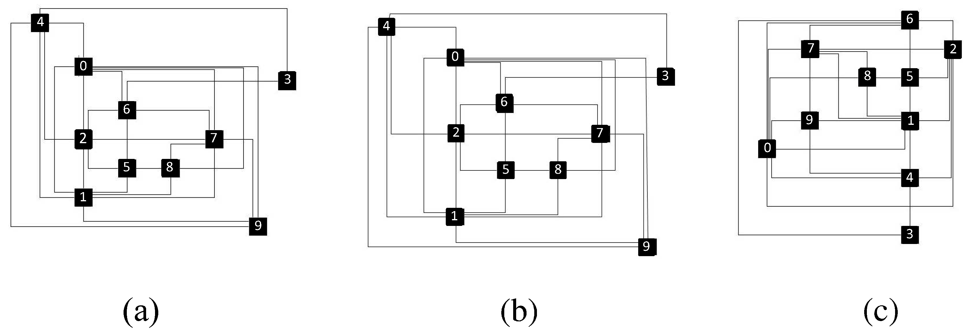
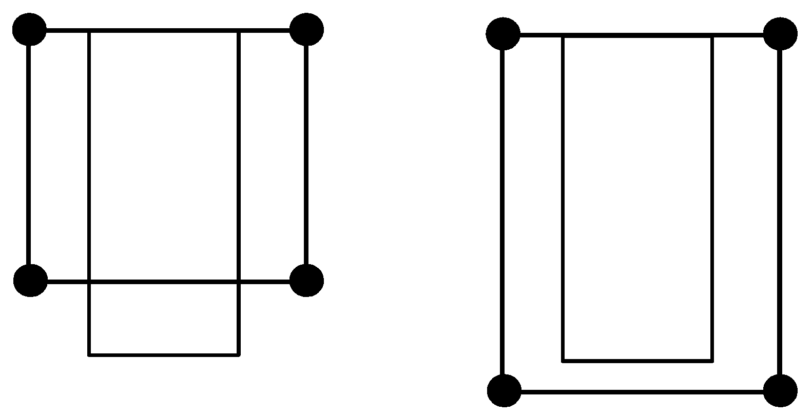
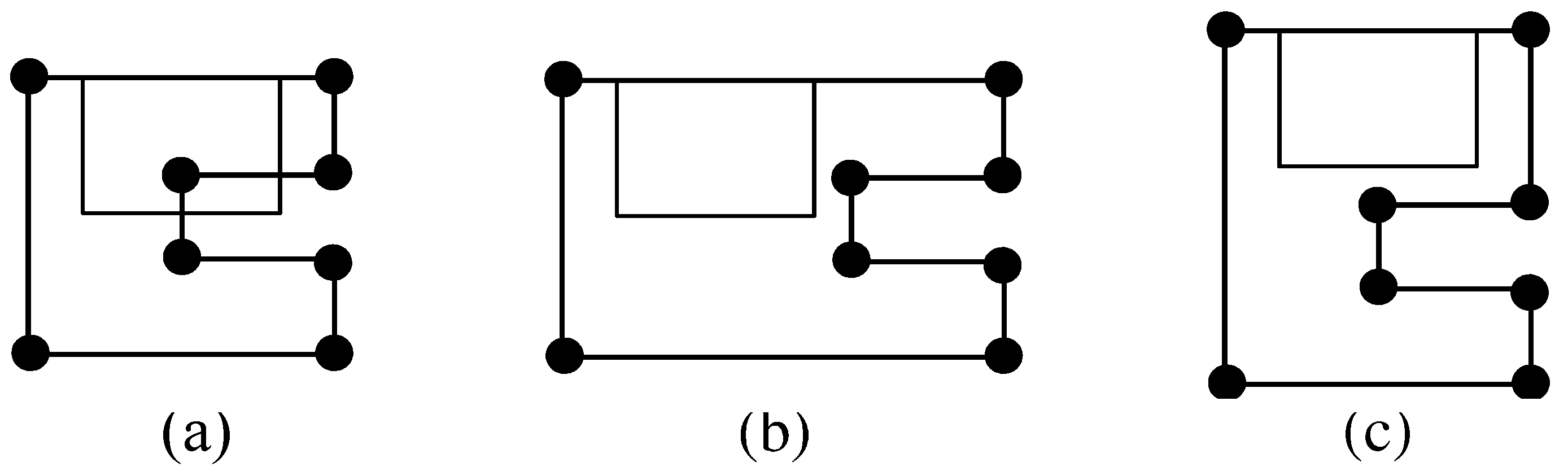
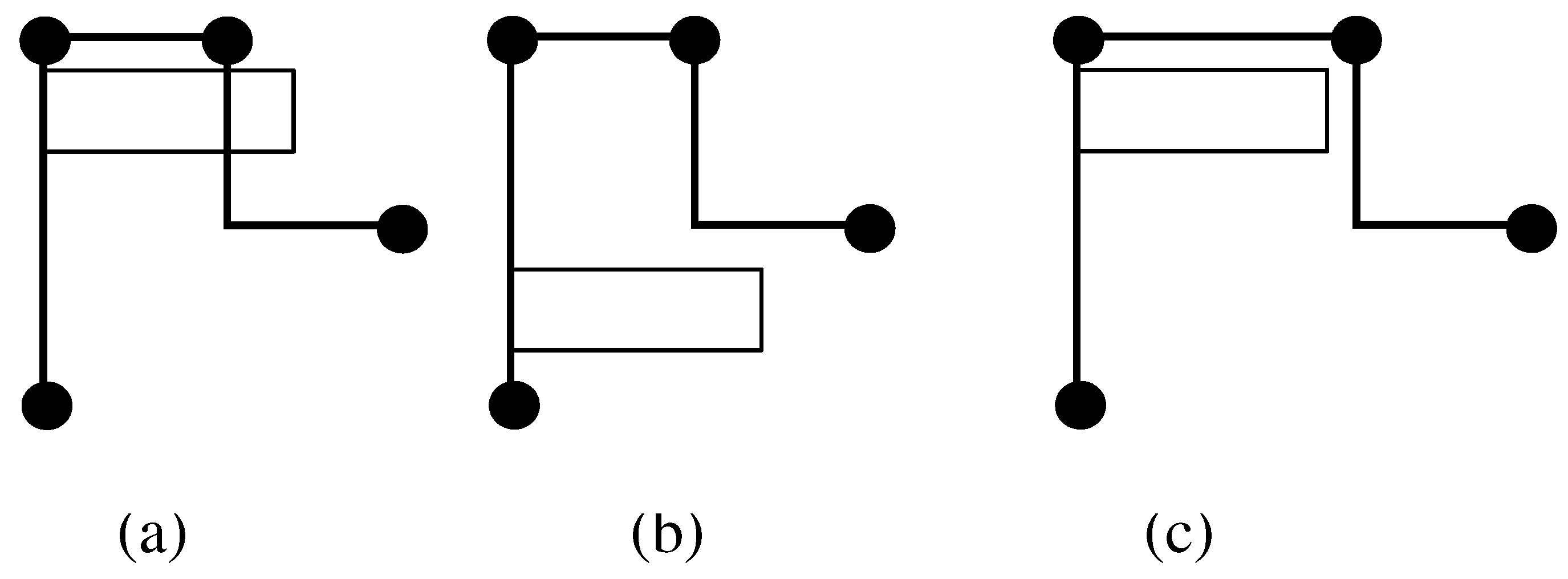
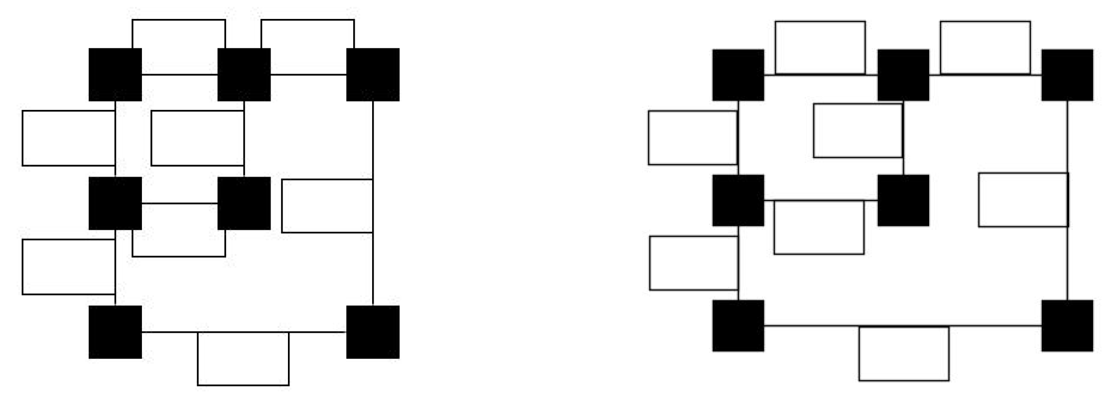
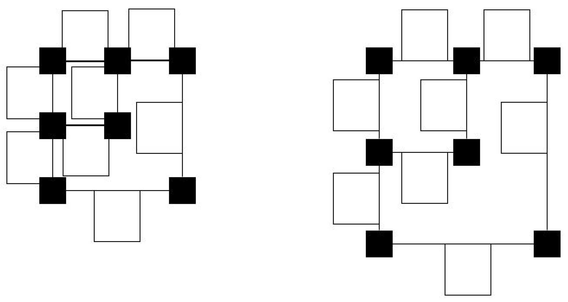
The notion of the mental map of a drawing has been introduced in [11]. By preserving the user’s mental map of a drawing, we generally mean that a user that has studied a drawing will not have to reinvest significant time and effort to visualize or understand the same drawing after some changes. For orthogonal drawings, we can preserve the mental map of a drawing by requiring that the orthogonal representation of a drawing remains the same after opening space. This is possible since an orthogonal representation of a graph G describes an equivalence class of planar orthogonal drawings of G with similar shapes [5]. In Figure 1 and Figure 2 we have orthogonal drawings of the same graph. The drawings in Figure 1a,b have the same orthogonal representation. It is obvious that both drawings have similar shapes, and the mental map between those two drawings is similar.
The problem we propose to solve is the following:
The opening space label placement problem:
Instance:
Given an orthogonal drawing with a label associated with each edge of the drawing.
Question:
Is there a label assignment where each edge has an overlap-free label assigned to it by minimally modifying the drawing?
This is a very challenging problem, since most of its variants are computationally hard, as we show in the next section.
4. Complexity Issues
First, we consider the more general case of the OSLP problem: Given an orthogonal drawing, increase its area minimally to achieve an overlap-free edge label assignment. This problem is NP-hard, which results from the fact that the problem of assigning labels to edges of a graph drawing, without increasing the area of the drawing, is NP-hard [12]. Hence, we have the following theorem:
Theorem 1.
The OSLP problem is NP-hard.
Next, we consider the following variation of the OSLP problem:
The Restricted Opening Space Label Placement (ROSLP) problem:
Instance:
Given an orthogonal drawing with a label associated with each edge of the drawing.
Question:
Is there a label assignment where each edge has an overlap-free label assigned to it without increasing the area of the drawing, while preserving its orthogonal representation?
In the ROSLP problem, the goal is to reroute the edges of the orthogonal drawing in order to assign overlap-free labels. In addition, we must not increase the area of the drawing, and we have to preserve the orthogonal representation of the drawing. Next, we prove that the ROSLP problem is NP-complete.
The NP-Completeness of the ROSLP Problem
We will prove that the ROSLP problem is NP-complete by transforming the three-partition problem [13], a well-known NP-complete problem, into it. Recall that the three-partition problem is defined as follows:
The three-partition problem:
Instance:
3m weights , a bound , such that for each i and such that .
Question:
Can the set be partitioned into m disjoint sets , , ..., , such that for all ? Note that each must contain exactly three elements.
In order to transform the three-partition problem into ROSLP, we do the following: We construct an orthogonal drawing Γ with edge labels that corresponds to the three-partition problem. The goal is to associate a solution of the three-partition instance with the existence of an overlap-free edge label assignment of Γ, while preserving the orthogonal representation and without increasing the area of Γ.
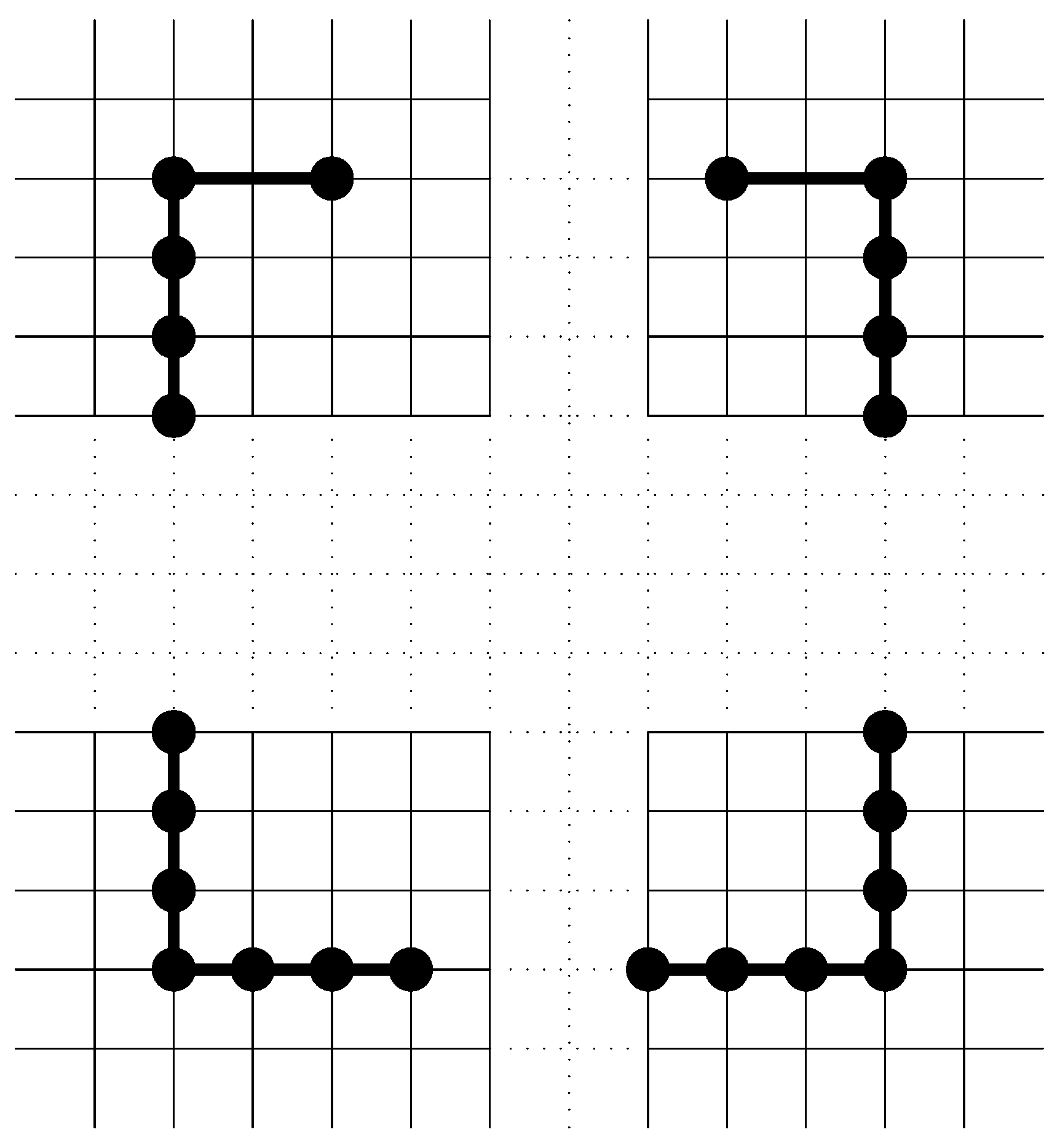
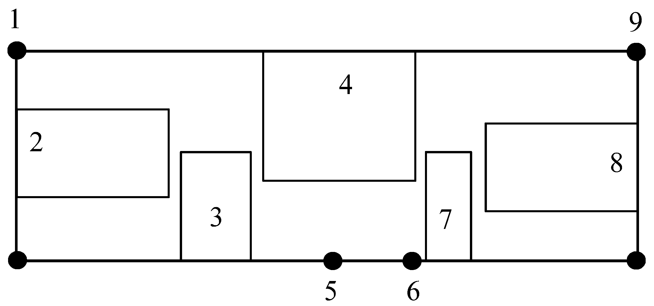
Next, we give an outline of our transformation. Given an instance p of the three-partition problem, we create an orthogonal drawing with edge labels corresponding to instance p in the following way: First, we construct a rectangular shape orthogonal drawing, which we call the skeleton drawing, as shown in Figure 3. There are nodes on each vertical side, nodes on the top horizontal side and nodes on the bottom horizontal side, where . Note that we cannot change the orthogonal representation and must preserve the area of the drawing; thus, the bounding rectangle of the skeleton drawing must not change.
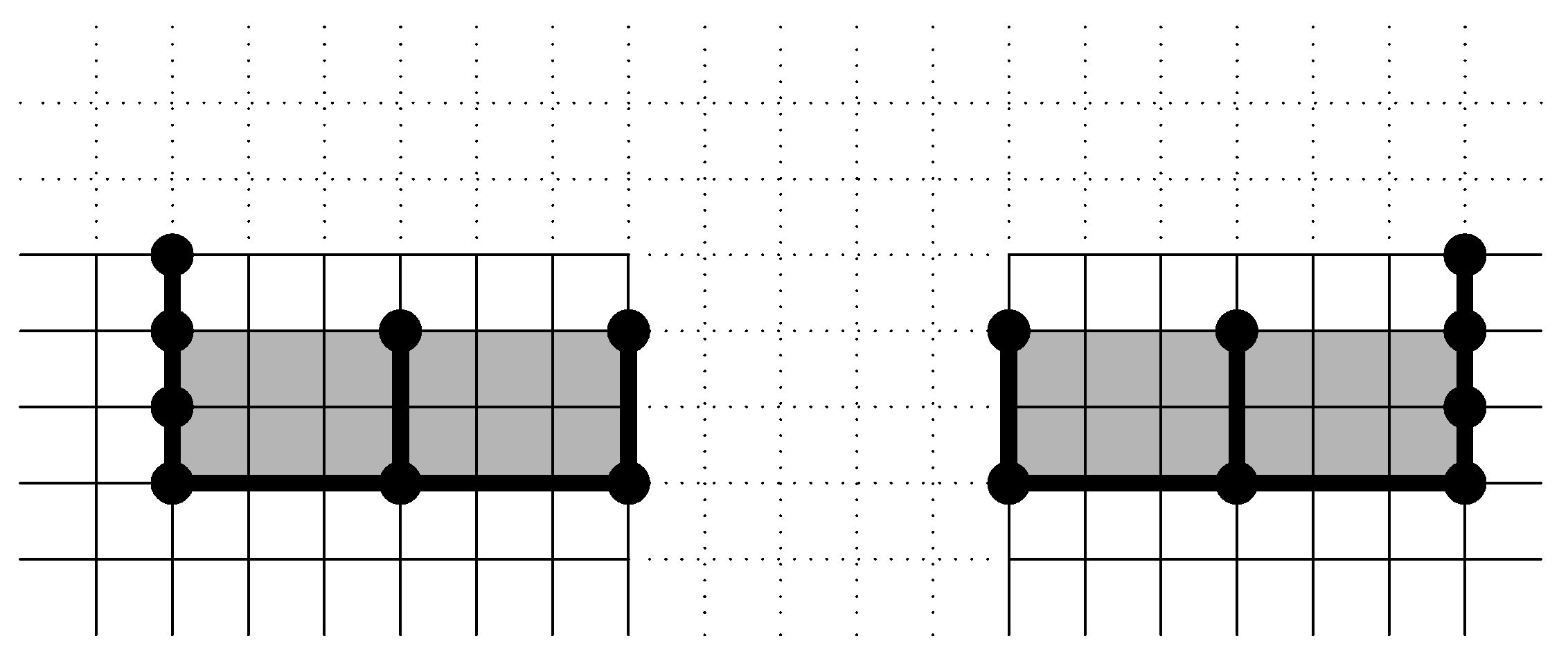
Next, we partition the bottom side of the skeleton drawing into m buckets, one for each of the three-set of a solution of the underlying instance p of the three-partition, by inserting nodes and edges in the bottom side of the skeleton drawing, as shown in Figure 4. Each of these edges will have length , and each bucket will have width .
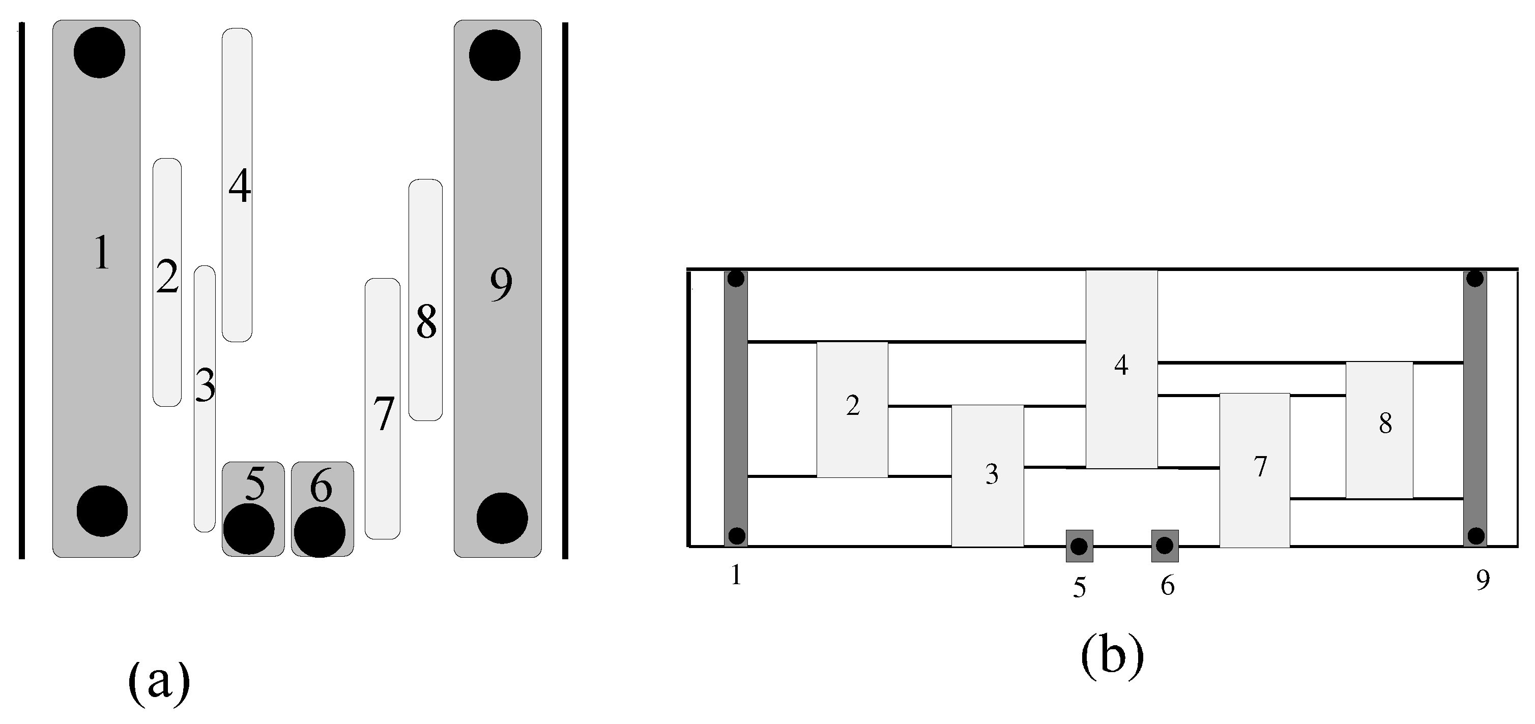
Next, we insert edges into the skeleton drawing. Each edge connects nodes of the opposite vertical sides of the skeleton drawing with the same y-coordinates. The top most edge connects the two nodes of the highest y-coordinate that are not part of the top horizontal side of the skeleton rectangle. We proceed from top to bottom until a total of edges have been placed. Each edge i has m U-shape bends, as shown in Figure 5.
Last, we assign a label to each of the edges we have inserted into the interior of the skeleton drawing. The label for edge i corresponds to the weight of the three-partition instance; it has width and height m. In addition, we assign a label of height and width K to each of the m edges of the top horizontal side of the skeleton rectangle.
To preserve the orthogonal representation and area of the orthogonal drawing Γ, while modifying Γ in order to assign overlap-free edge labels, we can only slide horizontally and/or stretch vertically the U-shapes of the edges, since we cannot alter the skeleton drawing. Thus, we have the following:
Fact 1.
We can modify the drawing only by sliding horizontally and/or stretching the U-shapes of the interior edges without creating any crossings.
Note that the drawing is a grid drawing; thus, two objects that do not overlap are separated by at least one unit.
Next, we will show that the orthogonal drawing Γ corresponding to an instance p of the three-partition has an overlap-free edge label assignment if and only if p has a solution.
Theorem 2.
The orthogonal drawing Γ that represents an instance p of a three-partition problem has an overlap-free edge label assignment if and only if p has a solution. Γ can be modified without increasing its area, while preserving its orthogonal representation, in order to find an overlap-free edge label assignment.
Proof:
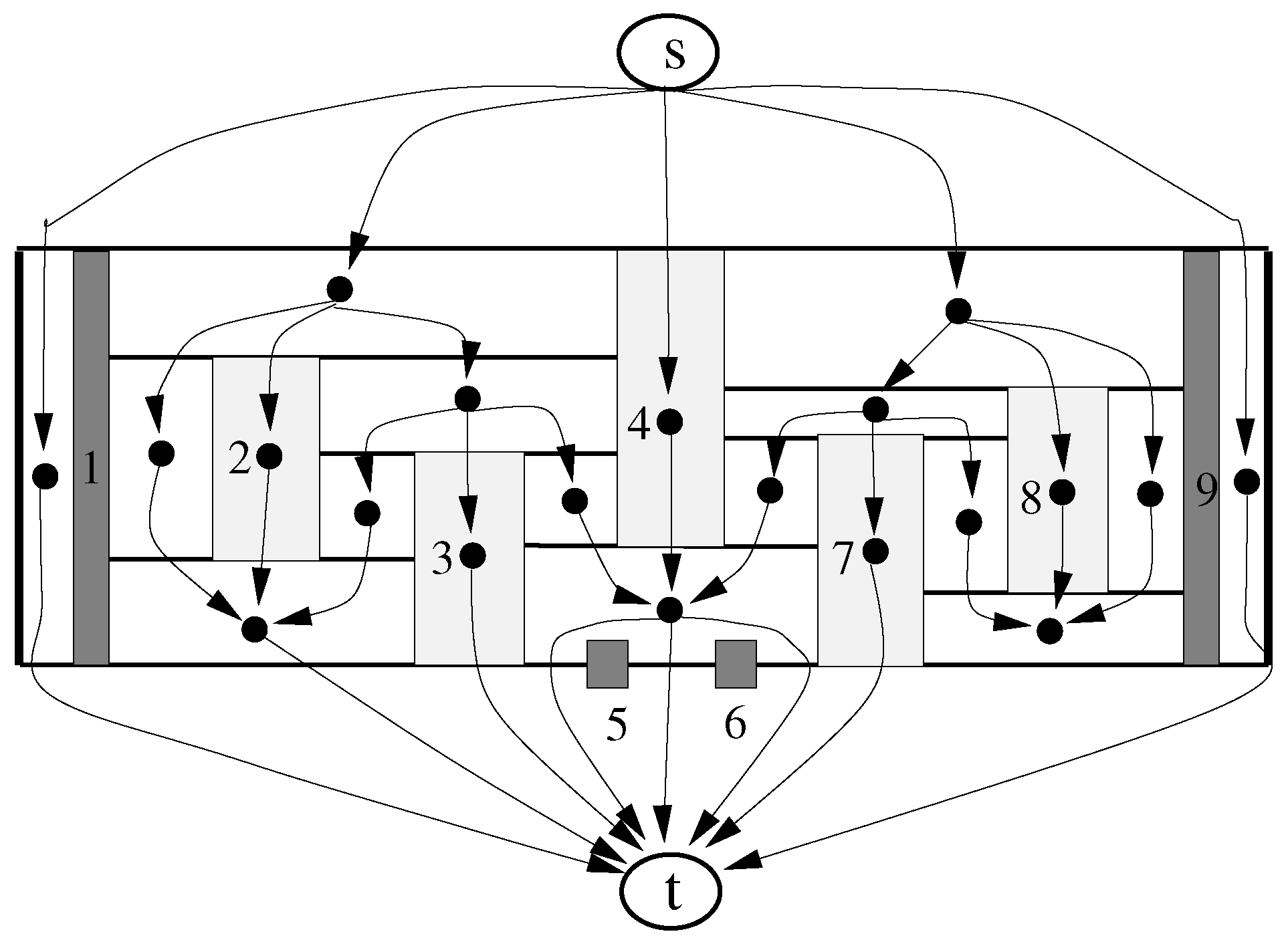
From the construction of the orthogonal drawing Γ, it follows that the label of each edge of the top horizontal side of the skeleton drawing, in order to be overlap-free, has to stretch exactly one U-shape bend from each edge below, as shown in Figure 6 (we call such a multilayer U-shape a super U-shape). Each super U-shape u has height ; thus, u must be inside some bucket in order to avoid overlaps, since the height of Γ is . Each super U-shape u has width . By construction, each bucket has width from which units are occupied by u and two units are used to separate the two vertical edges that define the boundaries of each bucket. Hence, there will be B free units of width in each bucket. This implies that at most one label of a top horizontal edge can be placed inside a super U-shape, since each label of a top horizontal edge has width K and .
The label of each interior edge i must be placed inside some bucket, since this is the only way to avoid overlaps; see Figure 7. Then, the width of a super U-shape will increase by .
By construction, there will be B free units of width in each bucket. Thus, a three-set of labels i, j and k fit exactly into a bucket if and only if the sum of , and is equal to B. Note that by definition , for each i, which implies that in each bucket, there can be at most three overlap-free labels, and because there are m buckets, it is trivial to conclude that each bucket must contain exactly three labels in order to have all labels free of overlaps. This implies that each label can fit into some bucket if and only if the weight of each set of three labels in each bucket is equal to B, which proves the theorem. ☐
The ROSLP problem, as stated, is in NP, and by Theorem 2, it is trivial to conclude that it is an NP-hard problem. Hence, we have the following theorem:
Theorem 3.
The ROSLP problem is NP-complete.
Because the OSLP problem is computationally hard, we must rely on heuristics to solve it. In the next section, we present such heuristics.
5. Heuristics for the OSLP Problem
In this section, we present a practical solution to the OSLP problem. Given an orthogonal drawing Γ, first we find an edge label assignment where overlaps are allowed by using existing techniques. Then, we modify Γ by locally blowing up part of the drawing (i.e., inserting rows and/or columns), so that the existing label assignment becomes overlap-free while preserving the orthogonal representation of the drawing. Next, we expand on the two main steps of our technique.
5.1. A Label Assignment with Overlaps
5.2. Resolving Overlaps
Given an orthogonal drawing Γ with labels assigned to each edge of Γ, we resolve label overlaps by increasing the height and/or width of Γ while preserving its orthogonal representation. From Section 4, where we present complexity results for the OSLP problem, it is clear that heuristics must be used to insert space to resolve overlaps for the OSLP problem.
Generally speaking, we will use a two-phase technique to resolve overlaps. During Phase 1, we resolve overlaps in the x-direction. Analogously, in Phase 2, we resolve overlaps in the y-direction. First, we define a partial order of all graphical features in the drawing (nodes, edges and labels). Next, we use plane sweep and flow techniques to find the minimum width and/or height needed to push apart objects in the drawing, so that all label overlaps are eliminated.
The OSLP problem has many similarities with the compaction problem in VLSI layout [16,17]. In both problems, the objective is to fit into the smallest area a set of geometric objects subject to a given set of constraints. The VLSI compaction problem is NP-complete, even if we allow objects to move only in one direction to resolve overlaps [16]. Actually, Lengauer [17] has pointed out that what makes the compaction problem computationally hard is that it is difficult to decide the partial order of two objects that overlap. We believe that this is what makes the OSLP problem hard, as well. Once a partial order for all objects is given, the compaction problem is solved in polynomial time if in addition objects are allowed to move only in one direction [16].
Next, we will show that the same holds true for the OSLP problem, as well. If the partial order of overlapping objects is given and labels in the drawing are allowed to move only in one direction (horizontal or vertical), then we can find the minimum area needed to resolve overlaps in polynomial time, while preserving the orthogonal representation of the input drawing. We will refer to it as the one-dimensional separation problem.
The one-dimensional separation problem:
Instance:
A drawing Γ with a label assignment with overlaps.
Question:
Increase the width (height) of Γ minimally, so that all overlaps in the x- (y-) direction are eliminated, while preserving: (i) the y- (x-) coordinates of all labels; (ii) the partial order of all the objects in Γ; (iii) the orthogonal representation of Γ.
We note the partial order of two objects i and j as when object i is to the left (respectively bottom) of j. In the one-dimensional separation problem, we do not allow parts of the drawing to be swapped in order to preserve the partial order, and we do not allow insertions of new bends or crossings in order to preserve the orthogonal representation. Generally speaking, the only action that is allowed is stretching the edges in the drawing such that we allocate space that allows overlapping labels to separate.
Next, we present two polynomial time algorithms for solving the one-dimensional separation problem. We will present the case where we increase only the width of the drawing to remove overlaps; the case of increasing the height is analogous.
6. Polynomial Time Algorithms for the One-Dimensional Separation Problem
First, we make the following assumptions to simplify our description:
- Labels are isothetic rectangles.
- The drawing is planar. If the drawing has crossings, then we insert a dummy node at each intersection and augment the input drawing to a planar one.
- We consider the separation of label overlaps in the x-direction. That is, we increase only the width of the drawing to resolve overlaps.
In the following sections, we present plane sweep and flow techniques for solving the one-dimensional separation problem.
6.1. The Plane Sweep Method
In order to solve the one-dimensional separation problem, we first define a partial order of all objects in the drawing (nodes, edges and labels). Then, we insert enough extra columns (horizontal space) between consecutive objects in the partial order, such that these objects are separated. Finally, we perform a compaction step in the drawing.
The task of defining the partial order of the objects in the drawing is not trivial, since an optimal partial order will produce an optimal solution for the OSLP problem. Recall that the input drawing is a planar or planarized graph. For each label, we define the following:
- The face of the drawing in which the label belongs.
- The edge segment to which the label is assigned.
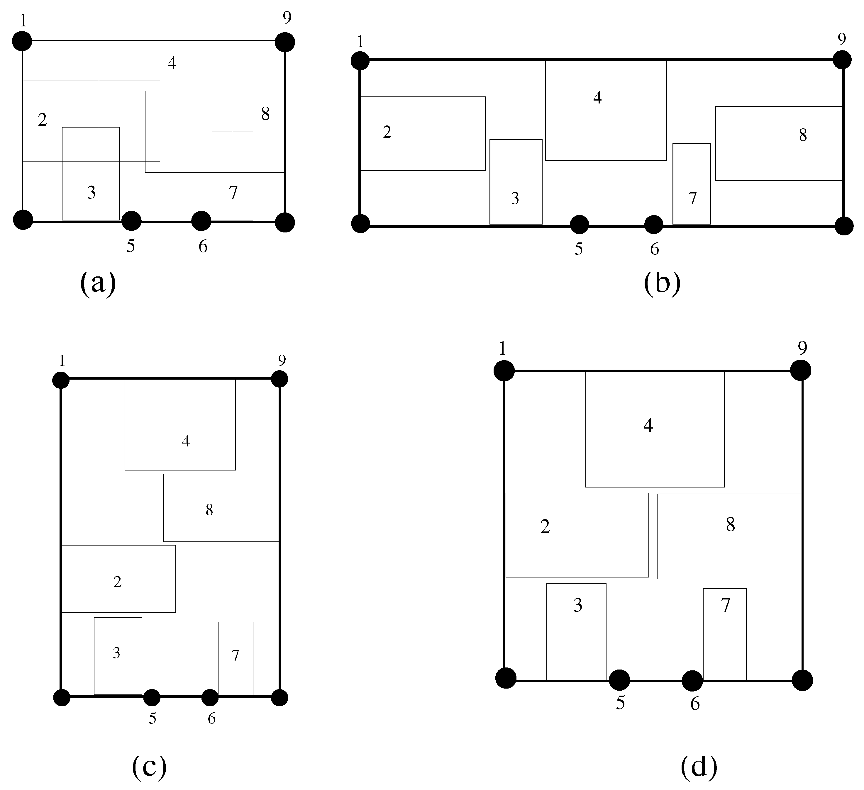
If a label overlaps more than one face of the drawing, then we place the label in the face where it overlaps the minimum area of other objects. An example is shown in Figure 8, where the label belongs to edge (2, 5), but it can be placed either to the left or to the right of edge (2, 5). The face to the left of edge (2, 5) is the preferred face to place the label since it is wider than the face to the right of edge (2, 5). Furthermore, as is shown in Figure 9, labels that overlap the boundaries of the face that they belong to are retracted inside that face.
A label is associated with one edge segment, in the case where an edge is composed of more than one segment. For example, in Figure 10, the label belongs to edge , which consists of the consecutive edge segments , , , and . Since we cannot change the y-coordinates of a label, the label can be either associated with the edge segment or .
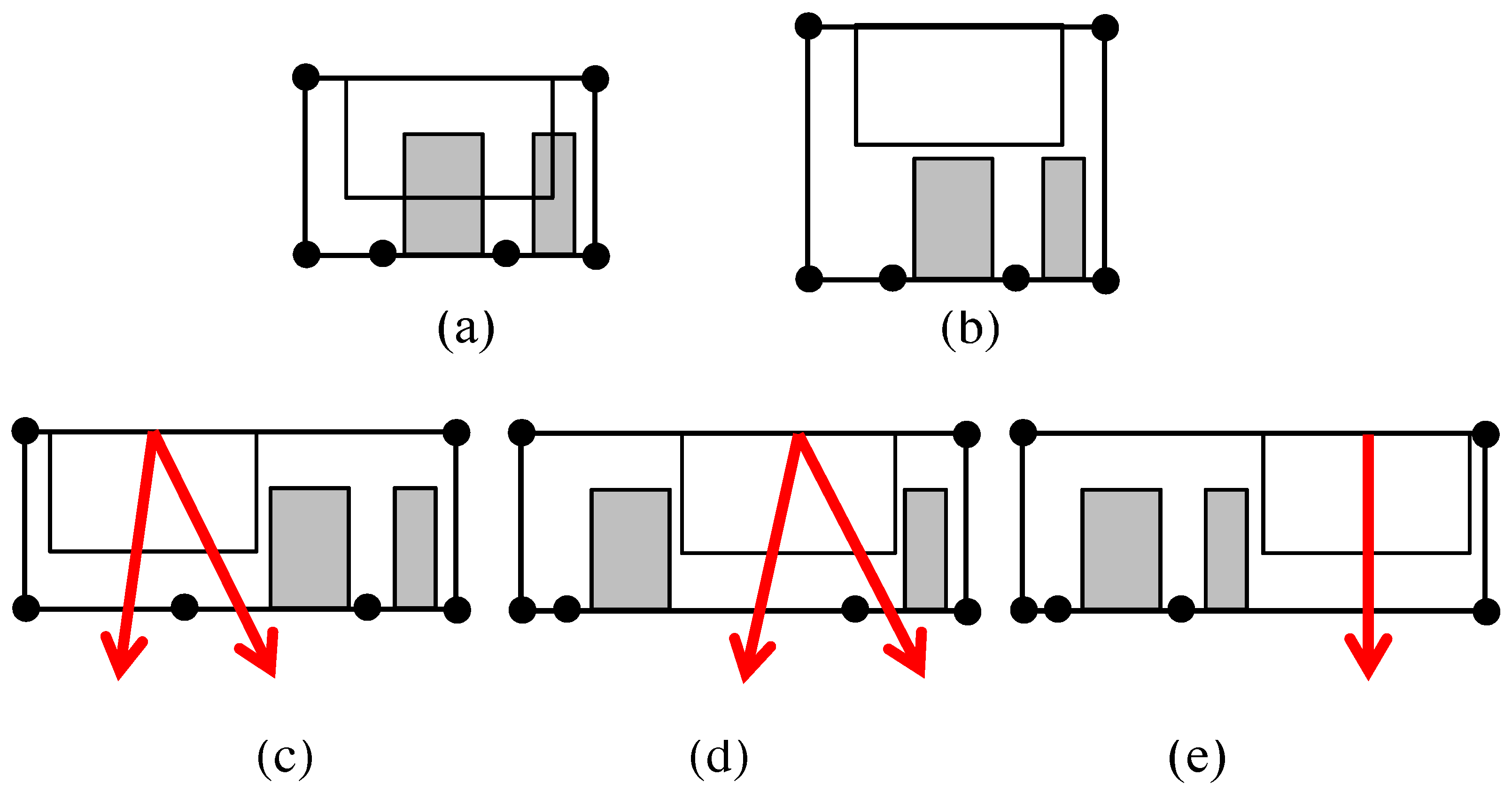
Before we assign the partial order of labels, we decide if we will resolve overlaps by increasing the width or height of the drawing. Actually, in some cases, overlaps can be resolved only by increasing the height (width) of the drawing. For example, in Figure 8, we have to increase the width, and in Figure 9, we have to increase the height in order to resolve label overlaps. In other cases, as shown in Figure 11 and Figure 12, we could increase the width or height of the drawing. Usually, we increase the height (respectively width) when labels have a greater overlap in the horizontal (vertical) direction.
Because we consider the case where we resolve label overlaps by increasing only the width of the drawing, we take into account only those labels that will become overlap-free by increasing the width of the drawing.
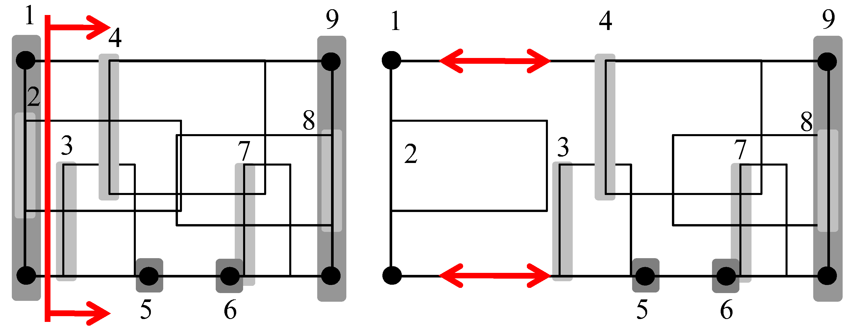
Now, we can assign the partial order of labels, nodes and vertical edge segments of the drawing. First, we associate each label with a vertical line segment (e.g., the left or right vertical side of the rectangle corresponding to the label). Then, we group nodes and vertical edge segments that are connected and share the same column in the drawing into single vertical objects, in order to preserve the orthogonal representation of the drawing; see Figure 13. Next, we sweep the plane from left to right, and each time we encounter a vertical object for the first time, we place it at the end of a queue. The order in which we have placed each object in the queue reveals its position in the partial order. Note that a label to the right of its associated vertical edge goes after the edge into the queue.
Now, we perform a plane sweep of the drawing from left to right with a vertical line. Each time the sweep line touches a vertical segment corresponding to a label l, we insert columns to separate l from all objects to the right of the sweep line (i.e., we push to the right all objects that follow l in the partial order). By doing that, we ensure that we have eliminated all overlaps.
Note that we expand to the right all horizontal lines that the sweep line intersects. Furthermore, if a label is between two vertical edge segments connected to the same node, then we cannot insert columns to resolve overlaps, since the columns will stretch the node. Thus, we must move this label into a different position, in a preprocessing step, where we can resolve overlaps by expanding the drawing.
In Figure 14, Figure 15, Figure 16 and Figure 17, we present the steps of the plane sweep algorithm that resolve the label overlaps of the orthogonal drawing shown in Figure 13.
One could improve the partial order of overlapping labels by rearranging their order. For example, as shown in Figure 12, different partial orders of overlapping labels produce different paths for the vertical space to be propagated through the drawing. Thus, in order to have efficient reuse of the vertical space inserted to resolve the overlaps, we place the top label, such that it has the minimum overlaps with other labels.
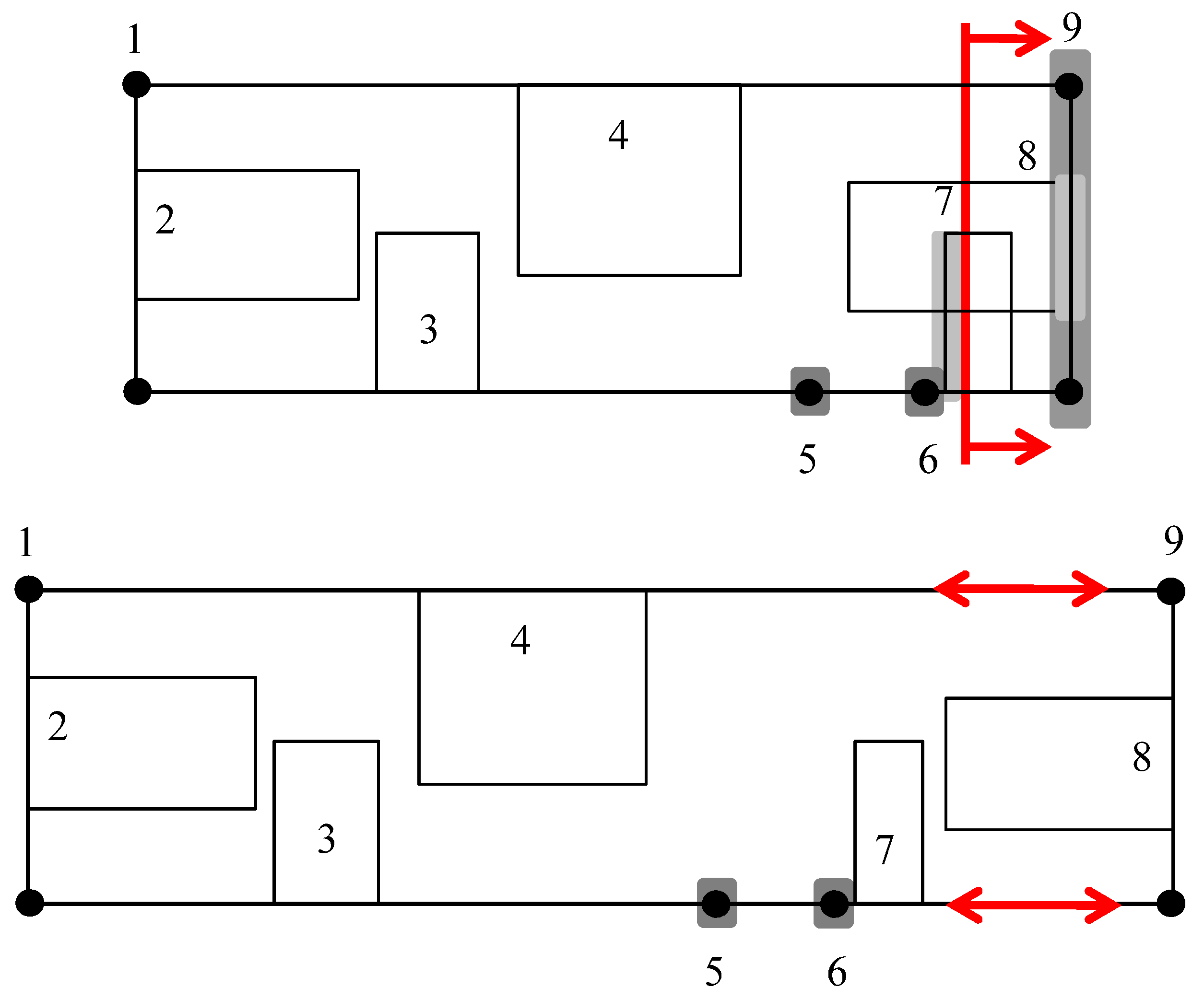
We have resolved overlaps by inserting extra columns between labels. It is easy to see that we could improve the solution by performing a VLSI compaction on the resulting drawing to minimize the width of the drawing; see Figure 18. Actually, by the plane sweep method, we have transformed the one-dimensional separation problem to its equivalent one-dimensional VLSI compaction problem. There are efficient techniques that optimally solve the one-dimensional VLSI compaction (i.e., compaction in one direction for objects with a predefined partial order) in polynomial time [16,17,18]. These techniques are based on the longest path method. It is trivial to conclude that the plane sweep algorithm runs in time, where n is the number of vertices, k is the number of vertical edge segments of the orthogonal representation and l is the number of edge labels.
One weak point of the longest path method is that it has the tendency to push all objects towards one side. Thus, it produces not only drawings that have long edges, but also drawings that are very dense on one side, while space on the other side remains unused. This characteristic of the graph-based approach is acceptable in VLSI layout where legibility or aesthetics are not important considerations. However, in graph drawing, the aesthetic quality of a drawing is critical; thus, we must preserve the mental map of the drawing after inserting extra space to resolve label overlaps. Therefore, the above technique, even though it is very attractive since it is fast and simple, might not serve our purpose well after all. In the next section, we present a method that produces not only minimum width, but also minimum edge length and evenly-spaced drawings based on flow techniques.
6.2. The Flow Method
In this section, we use minimum flow techniques to find the minimum width needed to eliminate label overlaps in an orthogonal drawing Γ, given a partial order of overlapping objects, while preserving the orthogonal representation of Γ. The case of finding minimum height is analogous.
Generally speaking, we will create a directed acyclic graph that transfers flow from the top to the bottom of the drawing in order to insert extra vertical space to resolve horizontal overlaps. Intuitively, if two objects overlap, then we must push between them at least as much flow as the amount of their overlap in the x-direction. We create a digraph that captures all possible routes that we can push flow such that all horizontal overlaps are resolved.
Since we want to preserve the orthogonal representation of the drawing, we insert space in such a way that the path of the inserted space does not intersect any vertical edge segment. It is important to note that the space opened at the top of the drawing can be reused by objects below, and the goal is to maximize the reuse of the space.
First, we decompose the input drawing into vertical edge segments, nodes and labels. Next, we remove all horizontal edge segments. Then, we group nodes and edge segments that are connected and share the same column in the drawing into single vertical objects, in order to preserve the orthogonal representation of the drawing.
Next, we obtain the partial order of the objects (vertical objects, nodes and labels) in the decomposed drawing. Then, we create a special graph, which we call the separation visibility graph . We will use a plane sweep method similar to the one described in the previous section to find the partial order of the objects. We sweep the plane from left to right, and each time, we encounter an object for the first time we place it at the end of a queue. The order in which we have placed each object in the queue reveals its position in the partial order. Note that a label to the right of its associated vertical edge goes after the edge into the queue.
Then, we construct the separation visibility graph as follows: For each vertical segment and node of the decomposed input drawing, we insert a node in . For each edge label l, which is a rectangle, we insert two nodes and two horizontal edges in . The nodes correspond to the vertical sides of l and the edges to the horizontal sides of l. Next, we insert edges in by expanding (to the left and to the right) the horizontal sides of each node in until they touch another node of .
Figure 19a illustrates the ordered set of objects corresponding to the input drawing with overlapping labels shown in Figure 13a. The corresponding separation visibility graph is shown in Figure 19b. Notice that we add two vertical line segments (nodes in ), one to the left and one to the right of the set of ordered objects. By adding these two objects, we ensure that each face of the separation visibility graph is a rectangle.
Fact 2.
Each face of the separation visibility graph is a rectangle.
We assign a weight to each edge e of , which represents the minimum distance the two objects connected with edge e must be kept apart to avoid overlaps. We assign weights in the following fashion:
- Each edge that connects two overlapping objects has weight equal to the amount of overlapping between these objects in the x-direction plus one.
- Each edge that corresponds to a horizontal side of a rectangle that represents either a label or a node has weight equal to the width of that label or node.
- Each edge that connects an edge e of the original drawing to a label assigned to e has weight zero.
- Any other edge has weight one.
Next, we show how to create the graph from the separation visibility graph (see Figure 20):
- Insert into nodes s and t above and below, respectively, of .
- Insert into a node for each face of .
- Add edges into that connect two neighboring faces of that share a horizontal edge segment. Edges are directed towards the face with a smaller y-coordinate.
- Connect with edges node s to each face that has a horizontal segment visible from a horizontal line that intersects node s.
- Connect with edges each face that has a horizontal segment visible from a horizontal line that intersects node t to node t.
By the construction of the separation visibility graph and Fact 2 we can prove the following result:
Lemma 1.
Graph includes every possible path that can be used to open up space in the x-direction to resolve overlaps without changing the orthogonal representation of the input orthogonal drawing.
In order to find the minimum width needed to resolve overlaps, we assign a lower and upper capacity to each edge of . Notice that each edge in intersects an edge in the corresponding graph. Each edge in has lower and upper capacity equal to a pair of weights for the only edge in that intersects. We obtain the pair of weights for each edge in as follows:
- Each edge that connects two overlapping objects has lower weight equal to the amount of overlapping between these objects in the x-direction plus one.
- Each edge that connects an edge e of the original drawing to a label assigned to e has upper and lower weight zero.
- Each remaining edge, other than edges connecting two vertical sides of labels, has lower weight one.
- Each edge connecting the two vertical sides of a label has upper and lower weight equal to the width of the label.
- Each edge, other than those connecting two vertical sides of a label or each edge e of the original drawing to a label assigned to e has upper weight equal to .
Next, we show that the minimum flow of produces the minimum width expansion needed to resolve overlaps.
Theorem 4.
The minimum flow of gives the minimum width of the drawing, such that all overlaps are resolved in one direction, and the orthogonal representation of the drawing is preserved.
Proof.
The resulting drawing has the same orthogonal representation since we do not allow flow to cross vertical edges of the drawing.
By construction, for any pair of overlapping labels, there will be enough flow going through to push them apart; thus, the resulting drawing has no overlaps.
Let us assume that the minimum flow of does not produce minimum width. This means that we have inserted extra vertical space. Therefore, there exists a path in from source to sink that carries at least one unit of extra flow. This is a contradiction, since we have obtained a minimum flow for . ☐
Sophisticated techniques can solve the minimum flow problem in time [19,20], where n is the number of vertices and m is the number of edges of . The coordinates of the resulting orthogonal drawing can be easily obtained, since the flow in each edge of gives the offset of objects in the original drawing that the corresponding edge in the visibility graph connects.
6.3. Results and Discussion
Labeling of edges and nodes aims to communicate the attributes of these graph objects in the most convenient way. This requires that labels be positioned in the most appropriate places and follow some basic aesthetic quality rules [15]. In addition, for technical maps or drawings, additional sets of rules influence the preferred label positions. These rules depend on the particular application and follow user specifications. For example, a label of an edge that is relevant to its source node must be placed close to the source node to avoid ambiguity. Therefore, in order to resolve label overlaps (Figure 21a), we must insert vertical space (Figure 21c), even though we could relocate the label to eliminate overlaps without inserting extra space (Figure 21b).
One point that we must emphasize is that the framework of the flow technique, in addition to resolving overlaps, can produce high quality label placement with respect to user’s preferences and aesthetic criteria. For example, in order to keep or place an edge label close to its associated node, we could assign a constant value to the upper and lower capacity of the edge in the flow graph that separates the node from each associated edge label.
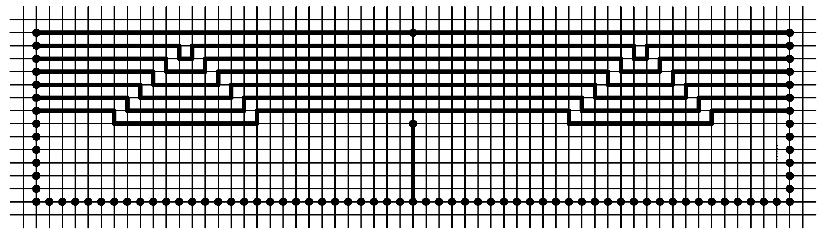
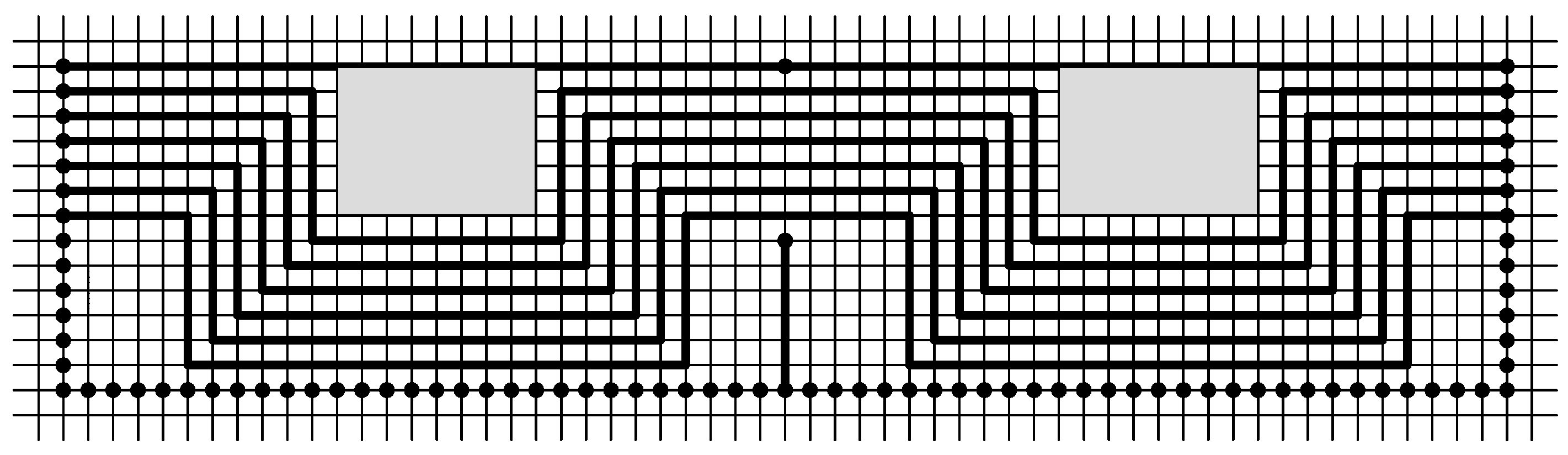
There are cases where overlaps of labels can be resolved by inserting extra space only in one direction. For example, in the orthogonal drawing shown in Figure 22, label overlaps can be resolved only by inserting vertical space. For the orthogonal drawings shown in Figure 2 and Figure 23, overlaps can be resolved only by inserting horizontal and vertical extra space. Furthermore, for the orthogonal drawing shown in Figure 24a, by running the algorithm once for each direction, we get better results. In Figure 24b, we resolve all overlaps in the x-direction; in Figure 24c, we resolve all overlaps in the y-direction; and in Figure 24d, we resolve overlaps of two objects in the direction that they intersect less. For example, if two objects overlap more horizontally than vertically, then we resolve overlaps by increasing the height of the drawing.
7. Conclusions
We have presented a comprehensive study of the problem of opening up space in a given drawing to assign labels to each object of a drawing with no overlaps. We showed that the OSLP problem is NP-complete, even for simple cases. We presented heuristics that assign labels to edges of orthogonal drawings. These methods can be trivially extended to assign labels to nodes and edges of an orthogonal drawing.
Author Contributions
Konstantinos G. Kakoulis and Ioannis G. Tollis contributed equally to this work.
Conflicts of Interest
The authors declare no conflict of interest.
References
- Kakoulis, K.G.; Tollis, I.G. Labeling Algorithms. In Handbook of Graph Drawing and Visualization; Tamassia, R., Ed.; Chapman and Hall/CRC Press: Boca Raton, FL, USA, 2013; pp. 489–515. [Google Scholar]
- Binucci, C.; Didimo, W.; Liotta, G.; Nonato, M. Orthogonal Drawings of Graphs with Vertex and Edge Labels. Comput. Geom. 2005, 32, 71–114. [Google Scholar] [CrossRef]
- Di Battista, R.; Didimo, W.; Patrignani, M.; Pizzonia, M. Orthogonal and Quasi-upward Drawings with Vertices of Prescribed Size. In Graph Drawing (Proc. GD 1999); Kratochvil, J., Ed.; Lecture Notes in Computer Science; Springer-Verlag: Berlin, Germany, 2000; Volume 1731, pp. 297–310. [Google Scholar]
- Klau, G.W.; Mutzel, P. Combining Graph Labeling and Compaction. In Graph Drawing (Proc. GD 1999); Kratochvil, J., Ed.; Lecture Notes in Computer Science; Springer-Verlag: Berlin, Germany, 1999; Volume 1731, pp. 27–37. [Google Scholar]
- Di Battista, G.; Eades, P.; Tamassia, R.; Tollis, I.G. Graph Drawing: Algorithms for the Visualization of Graphs; Prentice Hall: Upper Saddle River, NJ, USA, 1998. [Google Scholar]
- Tamassia, R. On Embedding a Graph in the Grid with the Minimum Number of Bends. SIAM J. Comput. 1987, 16, 421–444. [Google Scholar] [CrossRef]
- Di Battista, G.; Eades, P.; Tamassia, R.; Tollis, I.G. Algorithms for drawing graphs: An annotated bibliography. Comput. Geom. 1994, 4, 235–282. [Google Scholar] [CrossRef]
- Papakostas, A.; Six, J.; Tollis, I.G. Experimental and Theoretical Results in Interactive Orthogonal Graph Drawing. In Graph Drawing (Proc. GD 1996); North, S., Ed.; Lecture Notes in Computer Science; Springer-Verlag: Berlin, Germany, 1997; Volume 1190, pp. 371–386. [Google Scholar]
- Papakostas, A.; Tollis, I.G. Algorithms for Area-Efficient Orthogonal Drawings. Comput. Geom. 1998, 9, 83–110. [Google Scholar] [CrossRef]
- Papakostas, A.; Tollis, I.G. Issues in Interactive Orthogonal Graph Drawing. In Graph Drawing (Proc. GD 1995); Brandenburg, F., Ed.; Lecture Notes in Computer Science; Springer-Verlag: Berlin, Germany, 1996; Volume 1027, pp. 419–430. [Google Scholar]
- Misue, K.; Eades, P.; Lai, W.; Sugiyama, K. Layout Adjustement and the Mental Map. J. Vis. Lang. Comput. 1995, 6, 183–210. [Google Scholar] [CrossRef]
- Kakoulis, K.G.; Tollis, I.G. On the Complexity of the Edge Label Placement Problem. Comput. Geom. 2001, 18, 1–17. [Google Scholar] [CrossRef]
- Garey, M.R.; Johnson, D.S. Computers and Intractability: A Guide to the Theory of NP-Completeness; W. H. Freeman and Company: New York, NY, USA, 1979. [Google Scholar]
- Edmondson, S.; Christensen, J.; Marks, J.; Shieber, S. A General Cartographic Labeling Algorithm. Cartographica 1997, 33, 321–342. [Google Scholar]
- Kakoulis, K.G.; Tollis, I.G. A Unified Approach to Automatic Label Placement. Int. J. Comput. Geom. Appl. 2003, 13, 23–60. [Google Scholar] [CrossRef]
- Doenhardt, J.; Lengauer, T. Algorithmic aspects of one dimentional layout compaction. IEEE Trans. Comput.-Aided Des. Integr. Circuits Syst. 1987, 6, 863–879. [Google Scholar] [CrossRef]
- Lengauer, T. Combinatorial Algorithms for Integrated Circuuit Layout; Wiley-Teubner: New York, NY, USA, 1990. [Google Scholar]
- Hsueh, M.Y. Symbolic Layout and Compaction of Integrated Circuits. Ph.D. Thesis, University of California, Berkeley, CA, USA, 1979. [Google Scholar]
- Ahuja, R.K.; Magnanti, T.L.; Orlin, J.B. Network Flows: Theory, Algorithms, and Applications; Prentice Hall: Englewood Cliffs, NJ, USA, 1993. [Google Scholar]
- Orlin, J.B. A Faster Strongly Polynomial Minimum Cost Flow Algorithm. Oper. Res. 1993, 41, 338–350. [Google Scholar] [CrossRef]
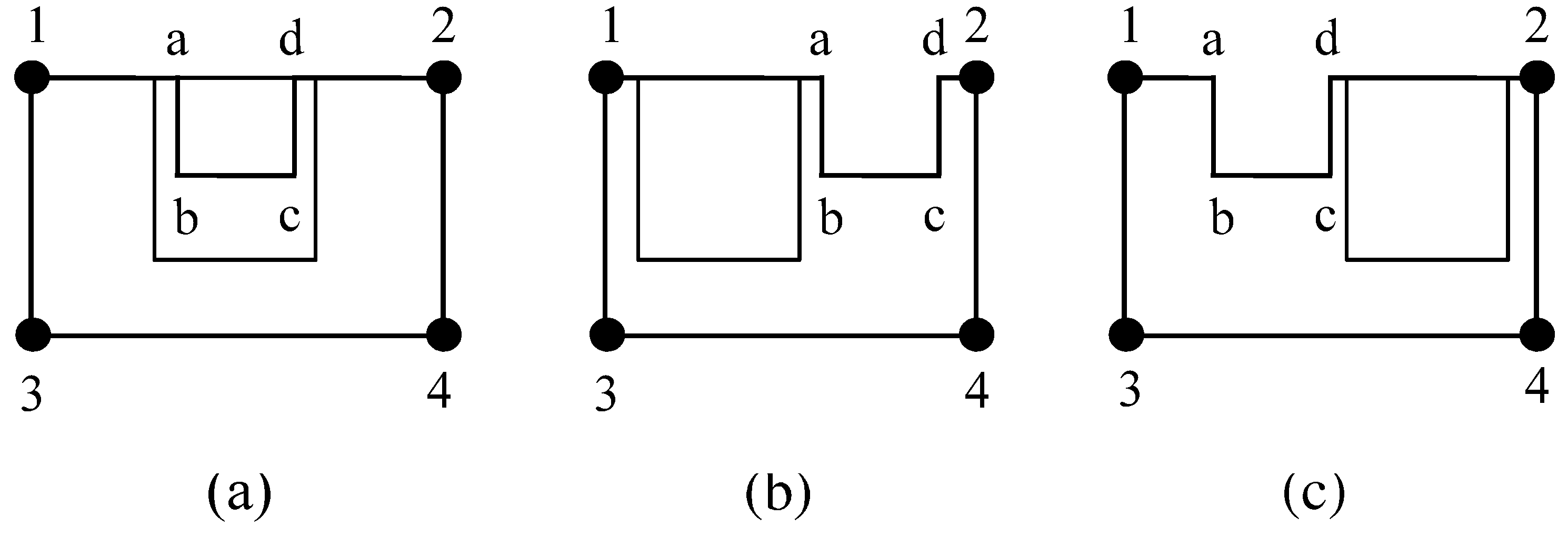
Figure 1.
Three orthogonal drawings of the same graph. Drawings (a,b) have the same orthogonal representation, while a drawing of a different orthogonal representation is shown in (c).
Figure 1.
Three orthogonal drawings of the same graph. Drawings (a,b) have the same orthogonal representation, while a drawing of a different orthogonal representation is shown in (c).

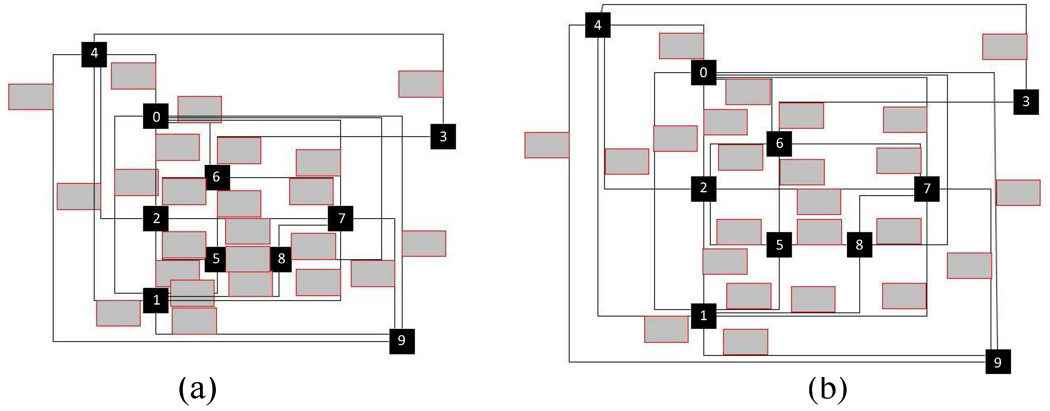
Figure 2.
(a) An orthogonal drawing with overlapping edge labels; (b) edge label overlaps have been resolved by inserting extra space using our flow technique.
Figure 2.
(a) An orthogonal drawing with overlapping edge labels; (b) edge label overlaps have been resolved by inserting extra space using our flow technique.

Figure 3.
The structure of the skeleton drawing.

Figure 4.
The buckets of the orthogonal drawing.

Figure 5.
The interior edges of the skeleton drawing, one edge for each of the elements of an instance of the three-partition problem.
Figure 5.
The interior edges of the skeleton drawing, one edge for each of the elements of an instance of the three-partition problem.

Figure 6.
The labels of the top horizontal edges and the U-shape bends of the edges below that stretch.
Figure 6.
The labels of the top horizontal edges and the U-shape bends of the edges below that stretch.

Figure 7.
A simple example of an orthogonal drawing corresponding to an instance of the three-partition problem with , , and weights .
Figure 7.
A simple example of an orthogonal drawing corresponding to an instance of the three-partition problem with , , and weights .
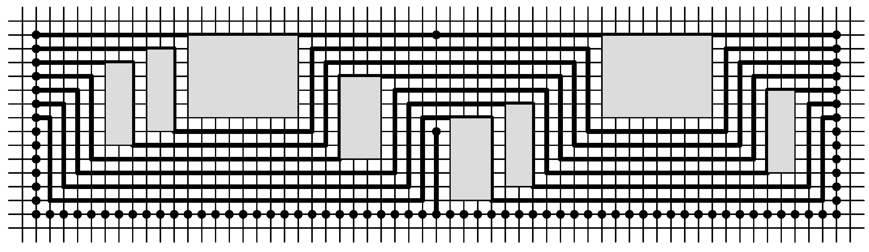
Figure 8.
A label that belongs to edge (2, 5) could be placed on either side of the edge.
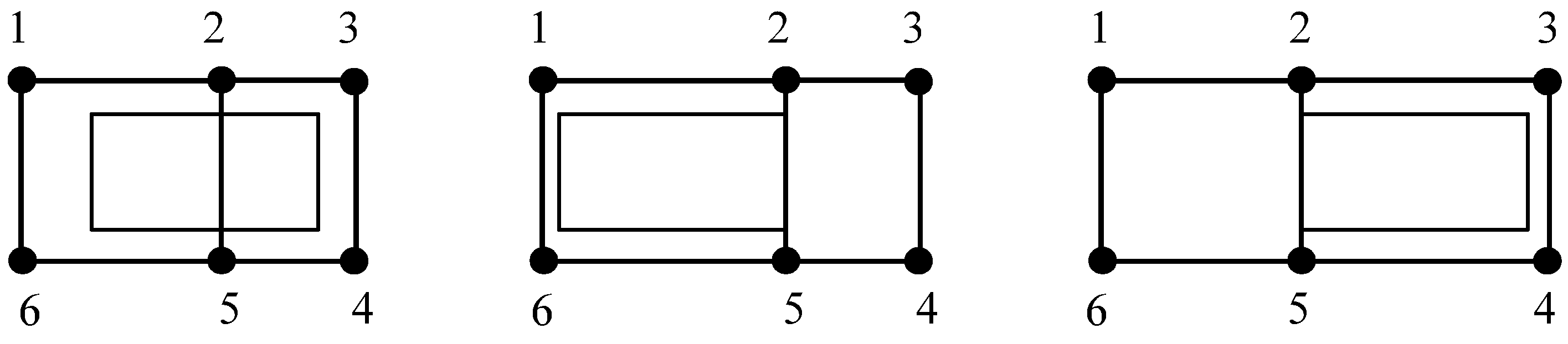
Figure 9.
An example where we must increase the height of the drawing to resolve label overlaps.

Figure 10.
(a) A label that can be assigned to more than one segment of the same edge. In (b,c) we show the two edge segments that the label can be placed.
Figure 10.
(a) A label that can be assigned to more than one segment of the same edge. In (b,c) we show the two edge segments that the label can be placed.

Figure 11.
(a) A case where a label overlaps part of the drawing; (b) position the label to resolve overlaps by increasing the width of the drawing; (c) position the label to resolve overlaps by increasing the height of the drawing.
Figure 11.
(a) A case where a label overlaps part of the drawing; (b) position the label to resolve overlaps by increasing the width of the drawing; (c) position the label to resolve overlaps by increasing the height of the drawing.

Figure 12.
(a) A complex case of overlaps; (b) we resolve overlaps by increasing the height of the drawing. In (c–e), we resolve overlaps by increasing the width of the drawing. In addition, all possible partial orders are presented, and the arrows show how the space will open.
Figure 12.
(a) A complex case of overlaps; (b) we resolve overlaps by increasing the height of the drawing. In (c–e), we resolve overlaps by increasing the width of the drawing. In addition, all possible partial orders are presented, and the arrows show how the space will open.

Figure 13.
(a) An input drawing with label overlaps; (b) each node, vertical edge segment and label is associated with a vertical object.
Figure 13.
(a) An input drawing with label overlaps; (b) each node, vertical edge segment and label is associated with a vertical object.

Figure 14.
The step of the plane sweep algorithm that resolves overlaps for Label 2.

Figure 15.
The step of the plane sweep algorithm that resolves overlaps for Label 3.
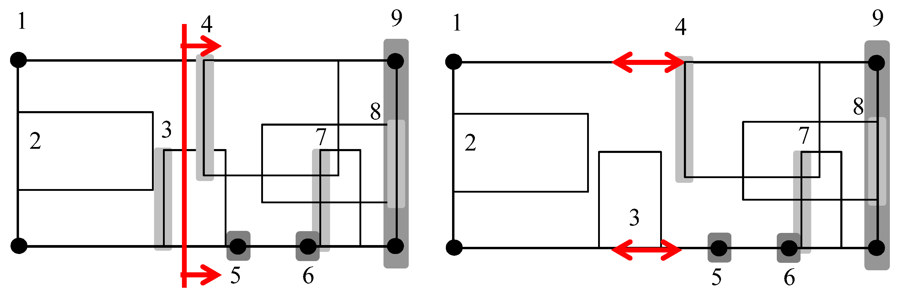
Figure 16.
The step of the plane sweep algorithm that resolves overlaps for Label 4.
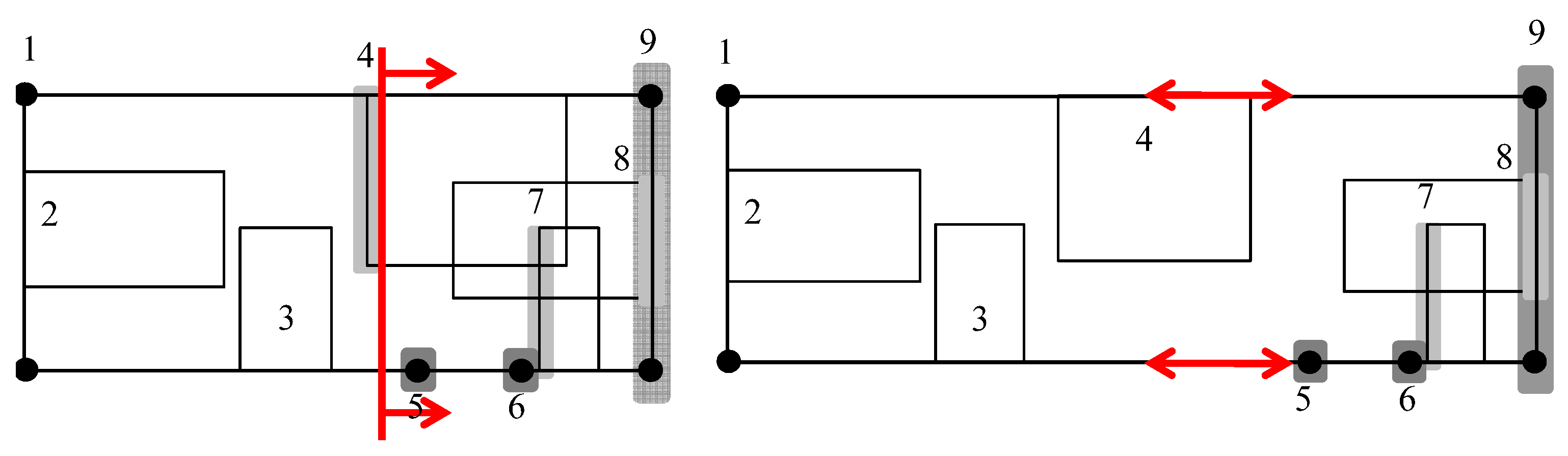
Figure 17.
The step of the plane sweep algorithm that resolves overlaps for Label 7.

Figure 18.
The compaction step of the plane sweep algorithm.

Figure 19.
(a) Ordered vertical objects; (b) their separation visibility graph.

Figure 20.
The flow graph of the separation visibility graph shown in Figure 19b.
Figure 20.
The flow graph of the separation visibility graph shown in Figure 19b.

Figure 21.
(a) An overlapping edge label, which is associated with the source (top) node; (b) the label is moved to eliminate overlaps without inserting extra space; (c) vertical space has been inserted to eliminate overlaps in order to avoid ambiguity.
Figure 21.
(a) An overlapping edge label, which is associated with the source (top) node; (b) the label is moved to eliminate overlaps without inserting extra space; (c) vertical space has been inserted to eliminate overlaps in order to avoid ambiguity.

Figure 22.
A sample orthogonal drawing where we resolve label overlaps by increasing only the width of the drawing.
Figure 22.
A sample orthogonal drawing where we resolve label overlaps by increasing only the width of the drawing.

Figure 23.
A sample orthogonal drawing where we have to increase the height and the width of the drawing in order to resolve label overlaps.
Figure 23.
A sample orthogonal drawing where we have to increase the height and the width of the drawing in order to resolve label overlaps.

Figure 24.
(a) A sample orthogonal drawing where we resolve label overlaps by increasing: (b) only the width; (c) only the height; and (d) the width and height.
Figure 24.
(a) A sample orthogonal drawing where we resolve label overlaps by increasing: (b) only the width; (c) only the height; and (d) the width and height.

© 2016 by the authors; licensee MDPI, Basel, Switzerland. This article is an open access article distributed under the terms and conditions of the Creative Commons by Attribution (CC-BY) license (http://creativecommons.org/licenses/by/4.0/).
Share and Cite
MDPI and ACS Style
Kakoulis, K.G.; Tollis, I.G. Modifying Orthogonal Drawings for Label Placement. Algorithms 2016, 9, 22. https://0-doi-org.brum.beds.ac.uk/10.3390/a9020022
AMA Style
Kakoulis KG, Tollis IG. Modifying Orthogonal Drawings for Label Placement. Algorithms. 2016; 9(2):22. https://0-doi-org.brum.beds.ac.uk/10.3390/a9020022
Chicago/Turabian StyleKakoulis, Konstantinos G., and Ioannis G. Tollis. 2016. "Modifying Orthogonal Drawings for Label Placement" Algorithms 9, no. 2: 22. https://0-doi-org.brum.beds.ac.uk/10.3390/a9020022
Note that from the first issue of 2016, this journal uses article numbers instead of page numbers. See further details here.