Artificial Neural Network Modeling for Predicting Wood Moisture Content in High Frequency Vacuum Drying Process

Abstract

The moisture content (MC) control is vital in the wood drying process. The study was based on BP (Back Propagation) neural network algorithm to predict the change of wood MC during the drying process of a high frequency vacuum. The data of real-time online measurement were used to construct the model, the drying time, position of measuring point, and internal temperature and pressure of wood as inputs of BP neural network model. The model structure was 4-6-1 and the decision coefficient R² and Mean squared error (Mse) of the training sample were 0.974 and 0.07355, respectively, indicating that the neural network model had superb generalization ability. Compared with the experimental measurements, the predicted values conformed to the variation law and size of experimental values, and the error was about 2% and the MC prediction error of measurement points along thickness direction was within 2%. Hence, the BP neural network model could successfully simulate and predict the change of wood MC during the high frequency drying process.

1. Introduction

Wood MC (moisture content) is one of the crucial indicators in the drying process as it has a direct impact on the stability of wood drying quality, and a reasonable control of MC can help in meeting the various quality requirements of actual wood products [1]. High frequency vacuum drying is a joint drying technology with a fast drying rate, low energy consumption, and low environmental pollution [2], and is in widespread use throughout the wood drying industry [3]. However, due to the interference of high frequency electromagnetic fields, the traditional MC online monitoring device cannot be used normally, which makes the online prediction and effective detection of wood MC problematic [4]. Therefore, the research on the prediction model of wood MC is of great significance in the high frequency drying process.

The wood structure is complex and it is difficult to establish a precise mathematical model through mathematical mechanism. An accurate control of MC requires precise mathematical models. The high frequency vacuum drying of wood is a non-linear, complex drying process, which is difficult to accurately express, control, or implement by using general mathematical methods [5]. The concept of BP (Back Propagation) neural network comes from the biological system of brain, which is composed of numerous neurons that are connected to each other through synapses that process information. The neural network has decent characteristics for predicting nonlinear complex systems [6,7], and the model reflects the intrinsic connection of experimental data after a finite number of iterative calculations. It is not only strong at processing nonlinearity, self-organizing adjustment, adaptive learning, and fault-tolerant anti-noise [8,9,10] but also can effectively deal with nonlinear and complex fuzzy processes. An effective network prediction model can be established without any assumption or theoretical relationship analysis, based on the historical data and powerful self-organization integration capabilities [11,12].

Artificial neural networks are increasingly being used for modeling in the field of wood science. For instance, in the field of wood drying, Avramidis (2006) [13] predicted the drying rate of wood based on neural network construction model; Zhang Dongyan (2008) [14] constructed a neural network model for predicting wood MC during conventional drying; İlhan Ceylan (2008) [15] used neural network models to study wood drying characteristics; Watanabe (2013, 2014) [16,17] employed artificial neural network model to predict the final moisture content of Sugi (Cryptomeria japonica) during drying and evaluate the drying stress on the wood surface. Ozsahin (2017) [18] utilized artificial neural networks to successfully predict the equilibrium moisture content and specific gravity of heat-treated wood. The artificial neural networks are widely used in the study of conventional drying characteristics, stress monitoring, and MC prediction of wood [19]; however, the use of neural networks to predict changes in the wood MC during high frequency drying has been rarely studied.

Hence, in order to provide a predictive model for the control of wood MC during high frequency drying, based on the BP neural network algorithm and using the real-time online measurement data, drying time, location of measuring point, and internal temperature and pressure of wood as the input to neural network model, the changes in the wood MC can be predicted. Also, the feasibility and prediction accuracy of the model was analyzed.

2. Materials and Methods

2.1. On-Line Monitoring of Wood Internal Temperature and Pressure

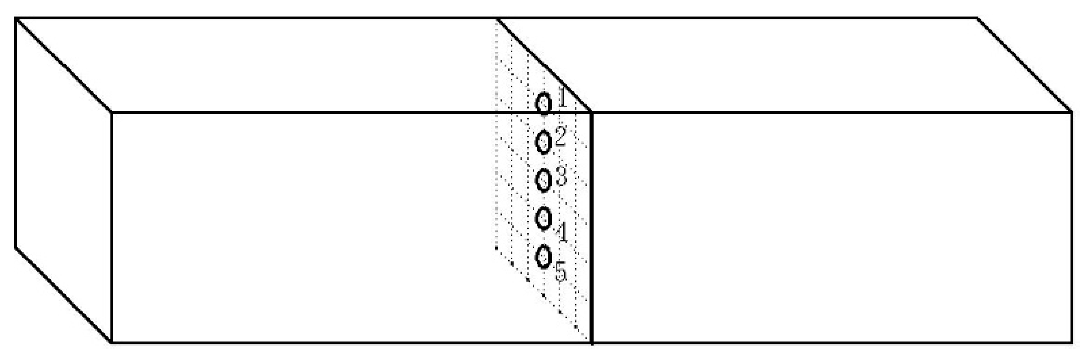
Some uniform and defect-free Mongolian pine (Pinus sylvestris var. mongholica Litv.) were selected. The 200 mm ends were removed at both ends of the test piece, and the specifications were 120 × 120 × 500 mm specimens after sawing and planning, and the initial moisture content was 50%. As shown in Figure 1, five temperature pressure measuring points were uniformly preset at the center of the sample in the thickness direction. Drilling holes on the side of specimen with a 4 mm drill bit to depth of 60 mm (seeing Figure 1 for specific locations). Each measuring point was embedded with one of the pressure and temperature fiber sensors, and the locations where the sensors were in contact with the surface of wood were coated with silica gel to ensure good sealing. The data was recorded online through the optical fiber sensors.

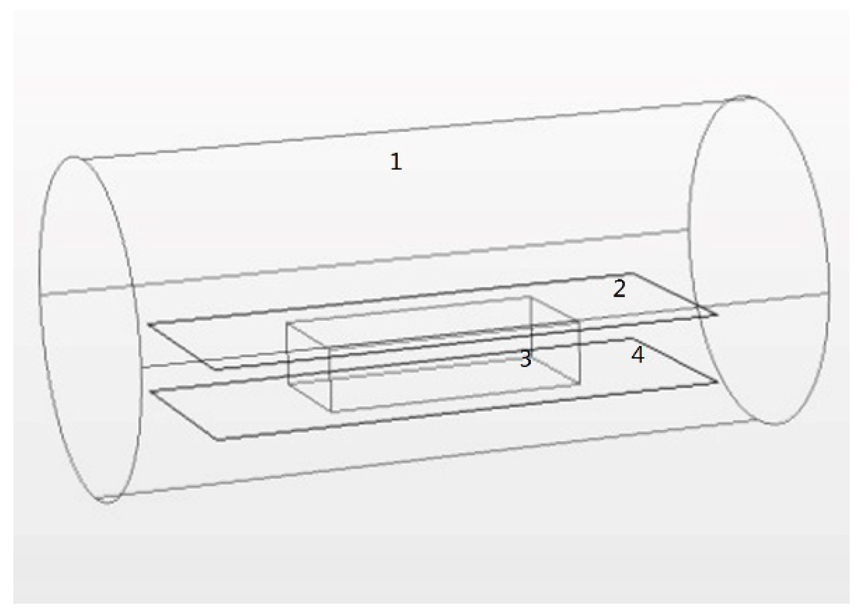
As shown in Figure 2, 1 is drying tank of high frequency vacuum with the diameter of 650 mm and length of 1350 mm; 2 and 4 are upper and lower plates respectively; and 3 is test material. The high frequency generator oscillates at the frequency of 27.12 MHz and outputs the effective power of 1 kW, which is powered by the center of electrode plate length.

During the drying process, the wood control temperature was set to 55 °C, the ambient pressure was set to 8 kPa, and the control of high frequency output time was set to stop for 2 min after a continuous oscillation for 7 min. In the early stage of drying, wood was quickly taken out and weighed after every 4 h, the real-time MC of wood was calculated, and the pressure and temperature values of five measuring points before the sample was taken out were recorded. In the middle stage of drying, the data were recorded once every 8 h; while, in the later stage of drying, the data were recorded once every 12 h.

The drying was carried out for 204 h until wood MC was dried to 11.56%. The experiment was stopped and a total of 135 data were recorded.

2.2. BP Neural Network Model

The BP (Back Propagation) model is currently the most studied and widely used artificial neural network model [20]. It has a powerful nonlinear mapping ability and the qualities of human intelligence such as self-learning, adaptive, associative memory, and parallel information processing. It can imitate the human brain nervous system to store, retrieve, and process the information with an excellent fault tolerance, and is extremely suitable for modeling and control of complex systems [21]. The Python language has a rich and powerful class library. It is an interpreted, interactive, and pure object-oriented scripting programming language that combines the best design principles and ideas of several different languages and is widely used in various fields of software development and application programming. Therefore, this paper built the BP neural network model using Python language programming.

2.2.1. Determination of Neuron Number

The neural network prediction model in this paper uses a three-layer feedforward network structure, which includes an input layer, a hidden layer, and an output layer [22]. The hidden layer can be further divided into a single hidden layer and multiple hidden layer according to the layer number. The multiple hidden layer is composed of multiple single hidden layers. Compared with a single hidden layer, a multiple hidden layer has a stronger generalization ability and higher prediction accuracy, but the training time is longer. The selection of hidden layers should be considered comprehensively based on the network accuracy and training time. For a simple mapping relationship, in case the network accuracy meets the requirements, the single hidden layer can be selected to speed up the process. For a complex mapping relationship, the multiple hidden layer can be selected to enhance the network prediction accuracy. Therefore, according to the research requirements, the study chose a single hidden layer.

The number of hidden neurons also has a certain impact on the network [23]. The neuron number in the hidden layer is directly related to the predictive power of network model. If the number is too high, it will not only increase the network training time but also the network will not converge to the target error, resulting in an over-fitting. If the number is too small, the model training will be insufficient and would not be able to completely express the relationship between the input variables and output parameters, thus affecting the predictive ability of the model. Therefore, the determination of neuron number in hidden layer is particularly critical [24].

The optimal neurons number was determined via trial and error method [5]. The neuron number in hidden layer was set to 4~10, and the learning error and epoch of different nodes were tested by network training. The optimal node was obtained by comparison analysis.

2.2.2. Data Normalization

The data obtained during the experiment were randomly divided into two data sets: a training group and a test group. The 101 test data of the training group accounted for 75% of the total data, while 34 data of the test group accounted for 25% of the total data.

Each input sample usually has different physical meanings and dimensions; hence, in order to make each input sample have an equally important position and also to prevent the adjustment of the weight into the flat area of error, the input sample needs to be normalized [5]. In addition, as the neurons of the BP neural network adopt the Sigmoid transfer function and the output is between [0, 1], it is also necessary to normalize the output samples (Equation (1)).

$$X^{\prime }=\frac{X-X_{\min }}{X_{\max }-X_{\min }}$$

(1)

where X’ is the X normalization value; X_max and X_min are the maximum and minimum values of X, respectively.

The neurons in each layer are only connected to the neurons in the adjacent layer and there is no connection between the neurons in each layer. Also, there is no feedback connection between the neurons in each layer. The input signal first propagates forward to the hidden node and then through the transformation function. The output information of the hidden node is propagated to the output node and the output result is given after processing. In general, the Sigmoid transfer function (Equation (2)) is used on all nodes of hidden layer. In the output layer, all nodes use the linear transfer function Pureline.

$$f=\frac{1}{1+e^{-x}}$$

(2)

where f represents the neuron output value and x represents the neuron input value.

2.2.3. Model Performance Analysis

In the model correlation test, the model was evaluated by using the determination coefficient R² and Mse (Mean squared error) of the training sample [25].

The determination coefficient R² is defined as:

$$R^2=\frac{{{\displaystyle {\sum }_{i=1}^n(t_i-p_i)}}^2}{{\displaystyle {\sum }_{i=1}^n{t}_i^2}{\displaystyle {\sum }_{i=1}^n{p}_i^2}}.$$

(3)

The Mean square error (Mse) is calculated as [12]:

$$Mse=\frac{1}{n}{\displaystyle \sum _{n=1}^n{(t_i-p_i)}^2}$$

(4)

where t_i (i = 1, 2, …, n) is the predicted value of the ith sample, p_i (i = 1, 2, …, n) is the true value of the ith sample, and n is the total number of all samples. The decision coefficient is in [0, 1], and the closer the value to 1, the better the model performance, and the closer to 0, the worse the model performance. The smaller the sample Mean square error, the better the prediction performance and the better the model performance. The learning efficiency is set to 0.01.

3. Results and Discussion

3.1. Determination of Neuron Number

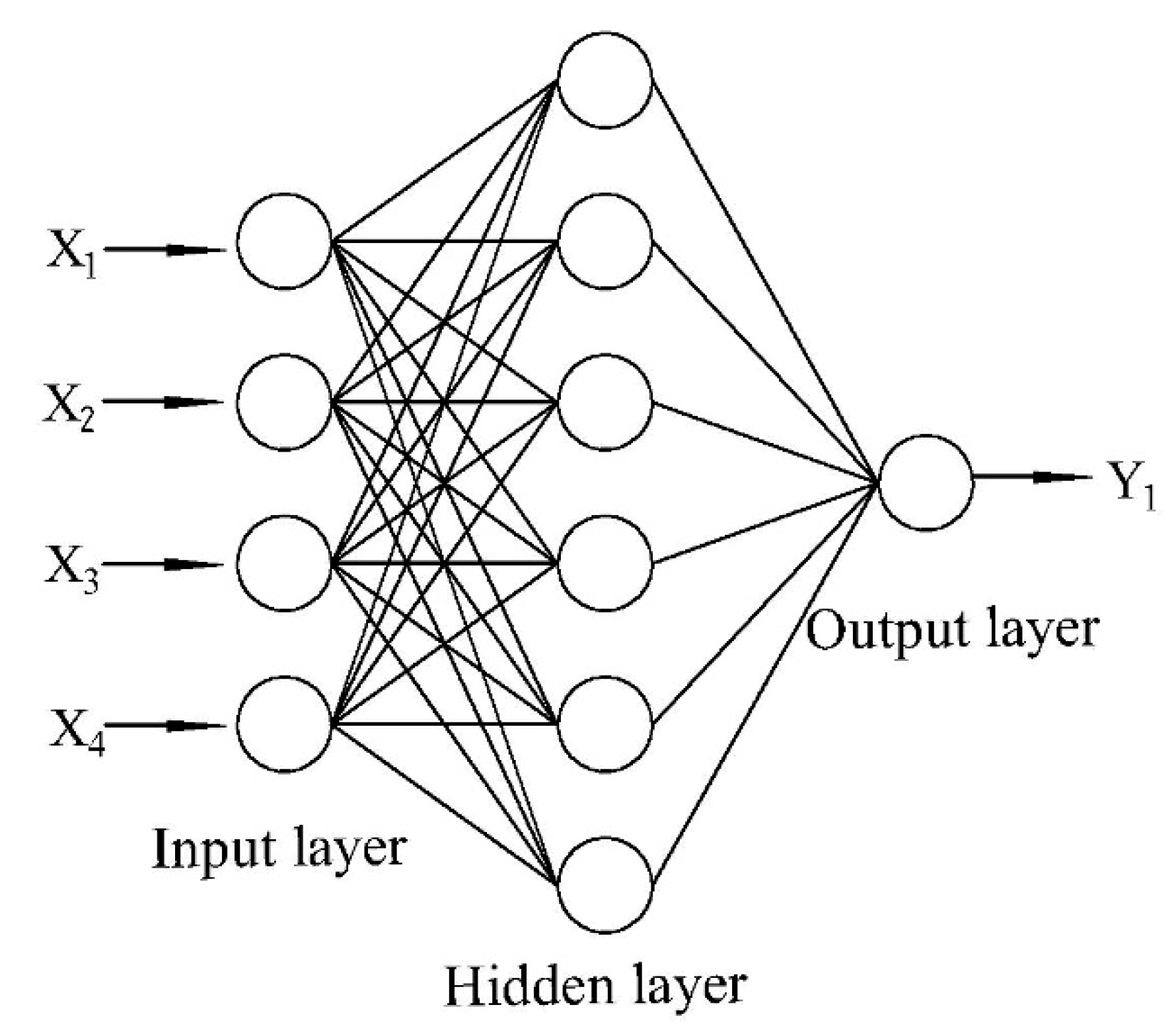
The corresponding relationship between the neuron number of hidden layer and the training error and epoch of neural network is shown in Figure 3. When the node number of hidden layer is 6, the training error is the smallest at 0.07355, and the epoch is 17, the network training is faster. These results show that the neural network model has superb generalization ability at this time [26]; hence, the node number of hidden layer is determined to be 6. According to the node number of hidden layer, the structure of neural network is shown in Figure 4.

3.2. Model Performance Analysis

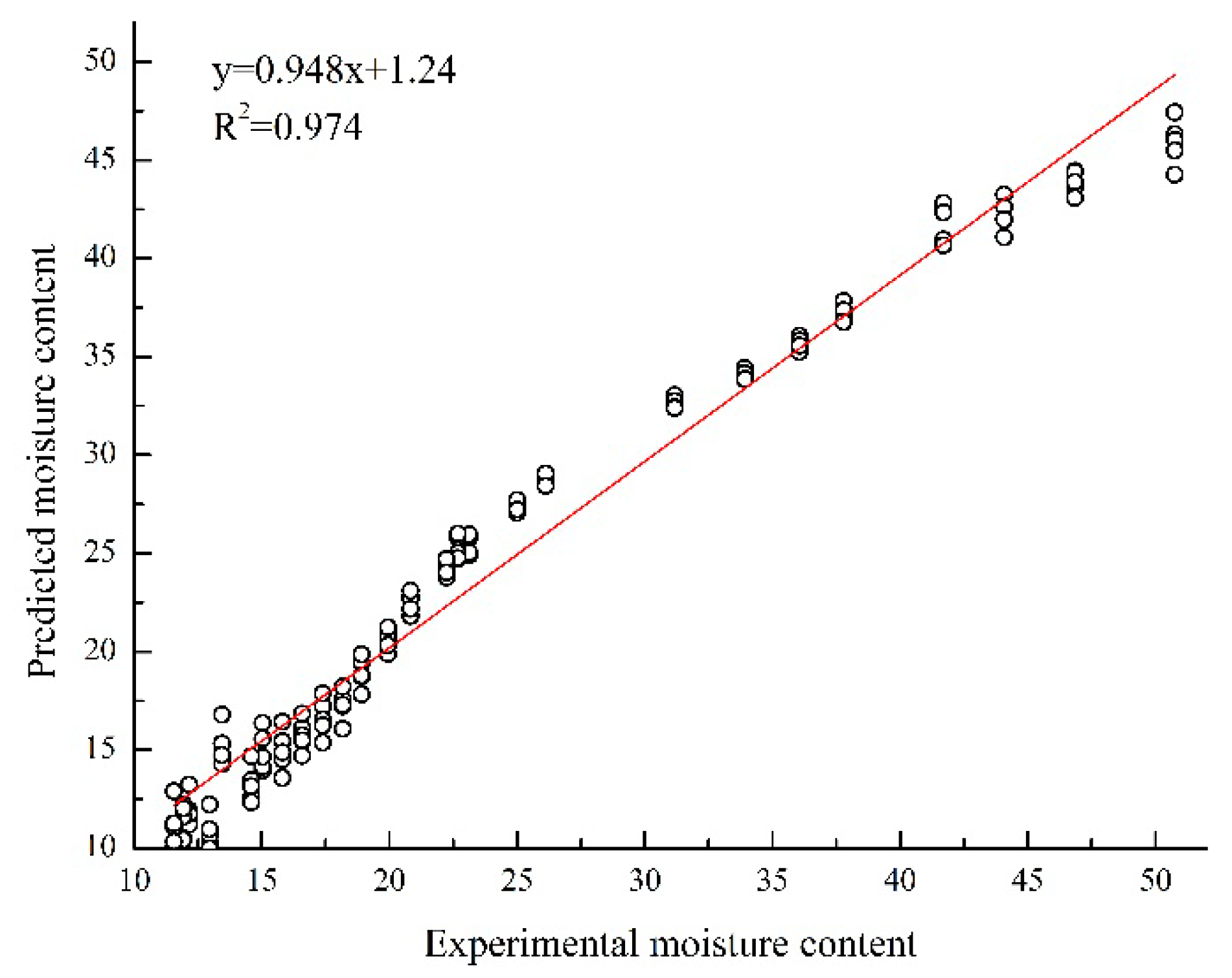
The training regression map for the BP neural network is shown in Figure 5. The linear regression equation between experimental and the predicted value is y = 0.948x + 1.24 while the determination coefficient R² is 0.974. These results indicate that the experimental and predicted values fit well. The BP neural network model has a good performance and can explain 97% of the above experimental values [24].

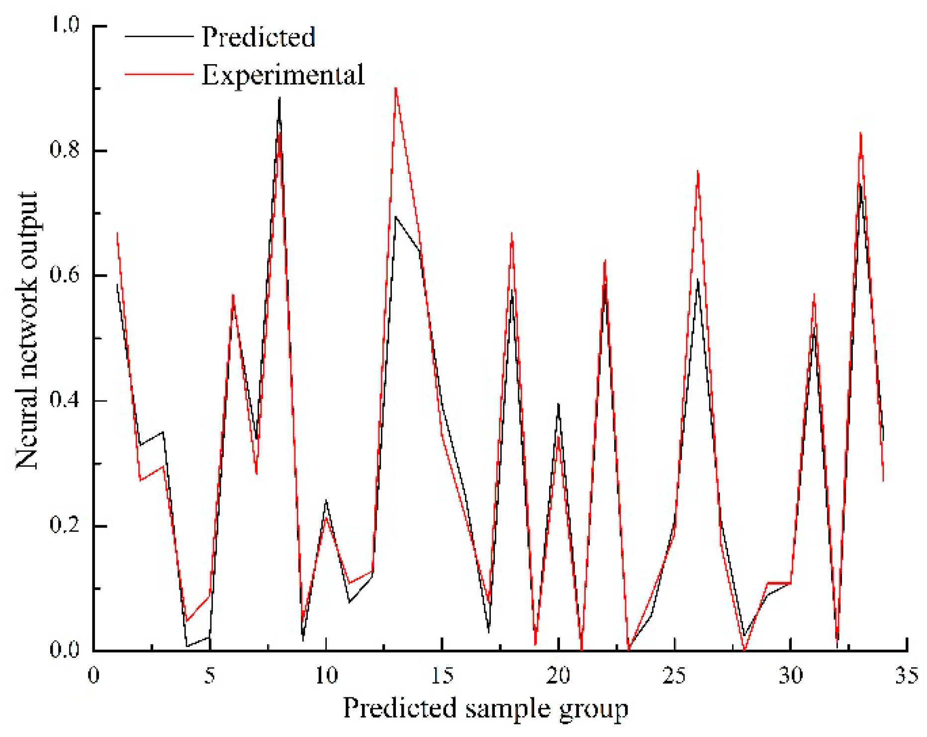
The predicted fitted curve for the neural network is shown in Figure 6. The remaining 25% of the samples are predicted and compared with the experimental values. The predicted values are consistent with the variation and size of the experimental values. Initially, the BP neural network model can simulate and predict the change of wood MC during high frequency drying.

3.3. Prediction of Moisture Content Change

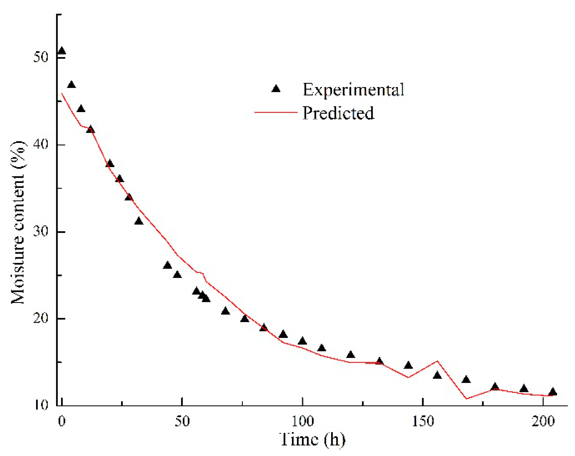
During the drying process of wood, the free water is primarily discharged along the large capillary system above the fiber saturation point. The bound water in cell wall is mainly discharged along the microcapillary system below the fiber saturation point. The bound water is affected by the hydroxyl interaction force in the amorphous region of cell wall [27]. In the early stage of drying, there is a short accelerated drying section. The energy of high frequency radiation is basically used to raise the temperature of wood, and the drying rate is gradually increased from zero. The middle stage of drying is constant-speed drying section. The energy of high frequency radiation is basically used to evaporate the moisture in wood. The MC decreases rapidly and exhibits constant-speed drying tendency. This stage basically completes the evaporation process of moisture in wood. In the later stage of drying, there is less water in wood, and the evaporation rate of moisture and the drying rate of wood gradually decrease [28].

The experimental data is input into the trained model for simulation verification. Figure 7 presents the curve of predicted and experimental values with time. In the early stage of drying, the predicted values are slightly lower than the experimental values; in the middle stage of drying, the predicted values are slightly higher than the experimental values; and in the later stage of drying, the predicted values have a slight wave motion, but overall the value is basically the same as the experimental values.

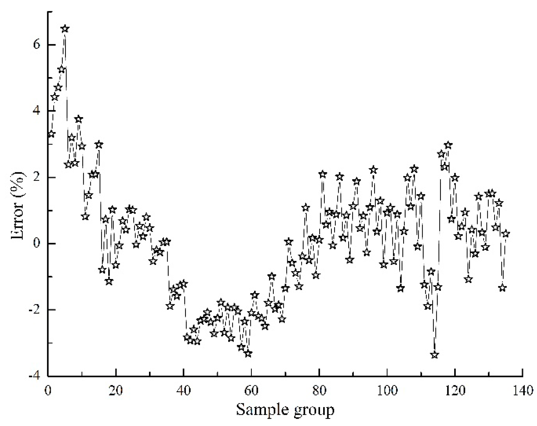
Figure 8 displays the predicted error curve for the neural network (error = experimental value − predicted value [29]). The overall error range is −4%~6% and most of the data is concentrated between −2%~2%, which can basically meet the requirements of prediction accuracy in wood drying.

Overall, the predicted data could basically reflect the change trend of MC during the high frequency drying process. The prediction error is about 2%, which proves the feasibility of BP neural network model in MC prediction. Moreover, if the external environmental parameters in the high frequency drying process and the relevant parameters of wood itself are known, the trained neural network model can be used to predict the MC change, thereby eliminating the complicated experimental detection process and saving time and cost [30].

3.4. Analysis of Stratified Moisture Content Prediction Error

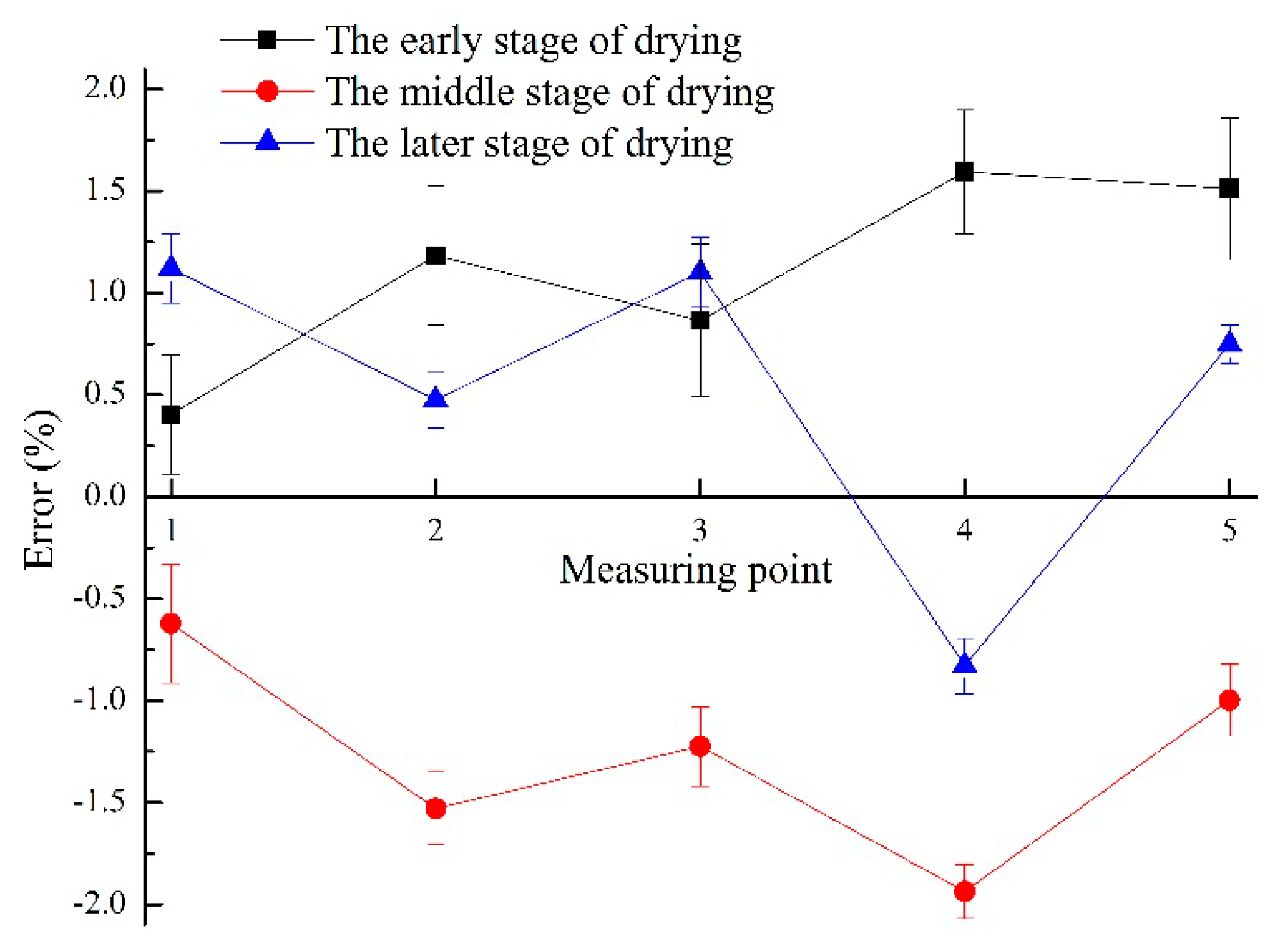
Figure 9 shows the MC prediction error of measurement points along thickness direction. In the early and later stage of drying, the error is positive and the predicted values are slightly less than the experimental values. In the middle stage of drying, the error is negative and the predicted values are slightly larger than the experimental values. Among these, the error in the middle stage of drying is the largest, followed by the early and later stage of drying. In the early and middle stage of drying, along the thickness direction of test material, from top to bottom, the error increases firstly, then decreases, then increases, and then decreases. The results show M-type trend with no clear law, and the error of the upper surface measurement point is the smallest. In the later stage of drying, along the thickness direction of the test material, from top to bottom, the error is firstly reduced, then increased, and then decreased, while the error at the upper intermediate layer is the smallest.

Due to the difference in material properties at different locations of the wood and the degree of electromagnetic radiation, the prediction accuracy of each measurement point is different. But overall, the prediction error of MC of each layer is less than 2%, indicating that the prediction accuracy of each measurement point is good and can meet the demand for stratified moisture content prediction.

4. Conclusions

The BP neural network was used to simulate the wood MC during the high frequency drying process. The drying time, the location of measuring point, and the internal temperature and pressure of the wood were taken as input variables, while the wood MC was the output variable, 101 test data of the training group accounted for 75% of the total data, while 34 data of the test group accounted for 25% of the total data. The results showed that when the number of hidden layer of neurons was six, the neural network training error was the smallest and the BP neural networks had better stability. The error between the predicted and the experimental values was about 2% and the stratified moisture content prediction error was within 2%, which the model could well simulate the change trend of wood MC during the drying process. In general, although the performance of wood varies greatly and the complex relationship has not been completely elucidated, the proposed neural network model is reliable and has a good predictive power.

References

- Xie, J. Study on Larch Wood Drying Models by Artificial Neural Network. Master’s Thesis, Northeast Forestry University, Harbin, China, 2013. [Google Scholar]
- Chai, H.J. Development and Validation of Simulation Model for Temperature Field during High Frequency Heating of Wood. Forests 2018, 9, 327. [Google Scholar] [CrossRef]
- Kong, F.X. Study on Technique of Radio-Frequency Vacuum Drying for Oak Veneer. J. Northeast. For. Univ. 2018, 6, 46. [Google Scholar]
- Li, X.J. Characteristics of Microwave Vacuum Drying of Wood and Mechanism of Thermal and Mass Transfer; China Environmental Science Press: Beijing, China, 2009; p. 65. ISBN 9787802099890. [Google Scholar]
- Yu, H.M. Study on Drying Mathematical Model of Hawthorn Using Microwave Coupled with Hot Air and Drying Machine Design. Ph.D. Thesis, Jilin University, Changchun, China, 2015. [Google Scholar]
- Zhou, P. MATLAB Neural Network Design and Application; Tsinghua University Press: Beijing, China, 2013; p. 153. ISBN 9787302313632. [Google Scholar]
- Poonnoy, P.; Tansakul, A. Artificial Neural Network Modeling for Temperature and Moisture Content Prediction in Tomato Slices Undergoing Microwave-Vacuum Drying. J. Food Sci. 2007, 72, E042–E047. [Google Scholar] [CrossRef] [PubMed]
- Sablani, S.S.; Kacimov, A. Non-iterative estimation of heat transfer coefficients using artificial neural network models. Int. J. Heat Mass Transf. 2005, 48, 665–679. [Google Scholar] [CrossRef]
- Rai, P.; Majumdar, G.C. Prediction of the viscosity of clarified fruit juice using artificial neural network: A combined effect of concentration and temperature. J. Food Eng. 2005, 68, 527–533. [Google Scholar] [CrossRef]
- Shyam, S.; Sablani, M. Using neural networks to predict thermal conductivity of food as a function of moisture content, temperature and apparent porosity. Food Res. Int. 2003, 36, 617–623. [Google Scholar]
- Hagan, M.T. Neural Network Design; PWS Publishing Company: Boston, MA, USA, 1996. [Google Scholar]
- Fu, Z. Artificial neural network modeling for predicting elastic strain of white birch disks during drying. Eur. J. Wood Wood Prod. 2017, 75, 949–955. [Google Scholar] [CrossRef]
- Wu, H.W.; Stavros, A. Prediction of Timber Kiln Drying Rates by Neural Networks. Dry Technol. 2006, 24, 1541–1545. [Google Scholar] [CrossRef]
- Zhang, D.Y. Neural network prediction model of wood moisture content for drying process. Sci. Silva Sin. 2008, 44, 94–98. [Google Scholar]
- İlhan, C. Determination of Drying Characteristics of Timber by Using Artificial Neural Networks and Mathematical Models. Dry Technol. 2008, 26, 1469–1476. [Google Scholar]
- Watanabe, K. Artificial neural network modeling for predicting final moisture content of individual Sugi (Cryptomeria japonica) samples during air-drying. J. Wood Sci. 2013, 59, 112–118. [Google Scholar] [CrossRef]
- Watanabe, K. Application of Near-Infrared Spectroscopy for Evaluation of Drying Stress on Lumber Surface: A Comparison of Artificial Neural Networks and Partial Least Squares Regression. Dry Technol. 2014, 32, 590–596. [Google Scholar] [CrossRef]
- Ozsahin, S. Prediction of equilibrium moisture content and specific gravity of heat treated wood by artificial neural networks. Eur. J. Wood Wood Prod. 2018, 76, 563–572. [Google Scholar] [CrossRef]
- Aghbashlo, M. Application of Artificial Neural Networks (ANNs) in Drying Technology: A Comprehensive Review. Dry Technol. 2015, 33, 1397–1462. [Google Scholar] [CrossRef]
- Zhang, Z.Y. Research on Load Forecasting Analysis of Wuhai Power Grid Based on Artificial Neural Network BP Algorithm. Master Thesis, University of Electronic Science and Technology of China, Sichuan, China, 2008. [Google Scholar]
- Bi, W. Research and Design of a Wood Drying Control System Based on Artificial Neural Network. Master’s Thesis, Jilin University, Changchun, China, 2011. [Google Scholar]
- MATLAB Chinese Forum. 30 Case Analysis of MATLAB Neural Network; Beijing University of Aeronautics and Astronautics Press: Beijing, China, 2010. [Google Scholar]
- Liu, T.Y. Improvement Research and Application of BP Neural Network. Master’s Thesis, Northeast Agricultural University, Harbin, China, 2011. [Google Scholar]
- Fu, Z.Y. Study on Dry Stress and Strain of Birch Tree in Conventional Drying Process. Ph.D. Thesis, Northeast Forestry University, Harbin, China, 2017. [Google Scholar]
- Zhang, T. Prediction Model of Moisture Content of Ginger Hot Air Drying Based on BP Neural Network and SVM. Master’s Thesis, Inner Mongolia Agricultural University, Hohhot, China, 2014. [Google Scholar]
- Xu, X. Nonlinear fitting calculation of wood thermal conductivity using neural networks. Zhejiang Univ. (Eng. Sci.) 2007, 41, 1201–1204. [Google Scholar]
- Gao, J.M. Wood Drying, 1st ed.; Science Press: Beijing, China, 2008; p. 10. ISBN 9787030205179. [Google Scholar]
- Allegretti, O. Nonsymmetrical drying tests—Experimental and numerical results for free and constrained spruce samples. Dry Technol. 2018, 36, 1554–1562. [Google Scholar] [CrossRef]
- Cai, Y.C. Wood High Frequency Vacuum Drying Mechanism; Northeast Forestry University Press: Harbin, China, 2007. [Google Scholar]
- Wang, Y. Prediction of Wood Moisture Content Based on BP Neural Network Optimized by SAGA. Tech. Autom. Appl. 2013, 32, 4–6. [Google Scholar]
Figure 1.
Diagram of the wood tested sample and location of the sensors. (1 is the upper layer measuring point; 2 is the upper middle layer measuring point; 3 is the core layer measuring point; 4 is the lower middle layer measuring point; and 5 is the lower layer measuring point).
Figure 2.
Drying tank of high frequency vacuum.
Figure 3.
Correspondence between the network error and the number of hidden layer neurons.
Figure 4.
BP (Back Propagation) neural network structure diagram (X1: drying time; X2: measuring point position; X3: temperature; X4: pressure; Y1: MC (moisture content)).
Figure 5.
Training regression graph of BP neural network.
Figure 6.
Prediction fitting curve of BP neural network.
Figure 7.
Simulation results of BP neural network.
Figure 8.
Prediction error of BP neural network.
Figure 9.
Error analysis of stratified moisture content prediction.
© 2018 by the authors. Licensee MDPI, Basel, Switzerland. This article is an open access article distributed under the terms and conditions of the Creative Commons Attribution (CC BY) license (http://creativecommons.org/licenses/by/4.0/).
Share and Cite
MDPI and ACS Style
Chai, H.; Chen, X.; Cai, Y.; Zhao, J. Artificial Neural Network Modeling for Predicting Wood Moisture Content in High Frequency Vacuum Drying Process. Forests 2019, 10, 16. https://0-doi-org.brum.beds.ac.uk/10.3390/f10010016
AMA Style
Chai H, Chen X, Cai Y, Zhao J. Artificial Neural Network Modeling for Predicting Wood Moisture Content in High Frequency Vacuum Drying Process. Forests. 2019; 10(1):16. https://0-doi-org.brum.beds.ac.uk/10.3390/f10010016
Chicago/Turabian StyleChai, Haojie, Xianming Chen, Yingchun Cai, and Jingyao Zhao. 2019. "Artificial Neural Network Modeling for Predicting Wood Moisture Content in High Frequency Vacuum Drying Process" Forests 10, no. 1: 16. https://0-doi-org.brum.beds.ac.uk/10.3390/f10010016
Note that from the first issue of 2016, this journal uses article numbers instead of page numbers. See further details here.